Article

Evaluating the Capability of Satellite Hyperspectral Imager, the ZY1–02D, for Topsoil Nitrogen Content Estimation and Mapping of Farmlands in Black Soil Area, China

1
College of Geo-Exploration Science and Technology, Jilin University, Changchun 130026, China
2
College of Surveying and Exploration Engineering, Jilin Jianzhu University, Changchun 130118, China
*
Author to whom correspondence should be addressed.
Remote Sens. 2022, 14(4), 1008; https://doi.org/10.3390/rs14041008
Submission received: 13 January 2022 / Revised: 8 February 2022 / Accepted: 17 February 2022 / Published: 18 February 2022
(This article belongs to the Special Issue Application of Hyperspectral Data in Ecological Environment)

Abstract

:
Soil nitrogen (N) content plays a vital role in agriculture and biogeochemical processes, ranging from the N fertilization management for intensive agricultural production to the patterns of N cycling in agroecological systems. While proximal sensing in laboratory settings can achieve ideal soil N estimation accuracy, the estimation and mapping by using remote sensing methods in a large spatial scale diplays low ability. A new hyperspectral imager with 166 spectral channels, the ZY1-02D, makes possible the detection of subtle but important spectral features of soil. This study aimed at exploring the capability of the ZY1-02D to estimate and map the topsoil N content of the black soil-covered farmlands in northeast China. To this aim, 646 soil samples from study sites were collected, processed, spectrally and geochemically measured for the soil N sensitive bands detection and partial least squares regression (PLSR) calibration and validation. The sensitive bands detection results showed an appealing regularity of the variability and stable tendency of the soil N sensitive spectral bands with the change of the sample size. Based on this, we compared the estimation capacity of the models developed with the full wavelength spectra and the models developed with the sensitive bands. The estimation based on ZY1-02D full wavelength spectral reflectance were robust, with R2 of 0.64 in validation. Further, the results of model developed with the sensitive bands showed better validation accuracy with R2 of 0.66 and were applied to create a map of topsoil N content of farmlands in the northeast China black soil area. The results demonstrated that sensitive bands modelling could enhance the accuracy of the estimation and simplify model, and what is more, showed the ideal capability of ZY1-02D for soil N content estimation at the regional scale.

1. Introduction

A valuable agricultural farmland resource, black soils [1,2,3], are suffering from degradation of soil fertility as a result of over-exploitation, soil erosion and the abuse of fertilizers in recent years, which seriously threatens the climate conditions and the food security of the world [4,5]. The capacity to achieve agronomic management optimization and intensive farming, and furthermore to achieve safe and sustainable development of agriculture partly depends on a better monitoring of soil nutrient contents [6,7]. The concentration of nitrogen (N) in the topsoil of farmlands is the main indicator of soil nutrient status [8], and the N fertilization is the important management intervention for intensive agricultural production [9,10,11]. Hence, how to estimate and map topsoil N content in black soil-covered farmlands is an essential research target for black soil resource protection and sustainable agricultural development.
Traditionally, the understanding of soil N content and its changes on a large spatial scale require extensive soil geochemical surveys. The high costs and low efficiency of soil surveys, commonly done by field sampling, remain a significant restriction on monitoring and mapping soil properties [12,13,14]. Therefore, it is necessary to develop and optimize more economical and effective techniques to estimate and map the N content of topsoil on a regional or even larger scale.
Since the launch of the first commercial satellite Earth Resource Technology Satellite (ERTS-1 a.k.a. Landsat-1) in 1972, the development of remote sensing techniques has made possible the rapid analysis of land cover in large areas [15,16]. From then on, increasing advances have been made in estimation and mapping soil properties by remote sensing techniques. The approach of analyzing the statistical relation of spectra and the certain property of object by calibration-validation strategy to provide quantitative estimation was built in 1968 [17], and then has been successfully applied in the quantitative analysis of soil properties (CaCO3, Fe2O3, Al2O3, CEC, pH, TN, SOC content, soil texture and soil moisture content etc.) after the 1990s [18,19,20,21,22,23].
The quantitative analysis of soil N content by the soil spectra, which are acquired from soil samples by proximal spectral measurements in a laboratory setting can commonly achieve ideal accuracies [19,24,25,26,27,28,29,30,31,32,33]. Table A1 provides a review of studies comparing soil N estimation using proximal and remote sensing methods. Several calibration-validation strategies have been employed in soil N content estimation by lab hyperspectral analysis after the 1990s, such as the multiple linear regression (MLR) [24], partial least squares regression (PLSR) [25], principle component regression (PCR) [19], and support vector machine (SVM) [31], which have obtained good to excellent R2 values (R2 = 0.92, 0.95, 0.85 and 0.58, respectively). Among them the partial least squares regression (PLSR) method has been proved the most effective and stable one in recent studies [25,26,27,28,29,30,31,32,33], as it takes advantage of the robust ability in the handling of multicollinearity and numerous noise sources in hyperspectral data [34,35].
However, the estimation accuracy of the N content of field soils was generally low when remote sensing spectroscopy data was applied [36,37,38,39,40,41,42,43], on account of the restrictions as the variability of the land cover, the spectral variation due to the atmospheric influence, the data uncertainty due to the variation of the temperature and the humidity on a large spatial scale, etc. [16,31,44]. Some efforts for soil N content estimation by remote sensing data (Landsat 5 TM, Landsat 8 OLI, Sentinel 1A, Sentinel 2A, etc.) have been reported in recent studies [38,39,40,41,42]. Due to the limitation of the available channels of these sensors, these studies usually apply black-box models as the BRT, RF, SVM, etc. with different algebraic indices to improve the estimation accuracy. However, when hyperspectral data (Hyperion, airborne CASI-SASI) have been employed in the estimation, the PLSR method could achieve better estimation results [36,37,43].
This study employed of the first time the data of a new space-borne hyperspectral imager, the ZY1-02D, in soil N content quantitative analysis modelling, to explore its potential for tsoil nitrogen content estimation on a regional spatial scale. The ZY1-02D advanced hyperspectral imager (AHSI) was lunched on 12 September 2019, and has the ability to acquire 166 bands of hyperspectral data with 30 m spatial resolution, 400–2500 nm spectral region and spectral resolution of 10 nm at VNIR and 20 nm at SWIR spectral region [45]. The continuous narrow hyperspectral bands of the data provide more detailed spectral information of the target soils and could make comparing the results of lab spectral analysis and its application in space-borne spectroscopy possible.
Additionally, even though previous studies have obtained ideal accuracies of the soil N content estimation, the models were usually unacceptable for other regions on account of the variation of the spectral statistical feature caused by the heterogeneity of samples [46,47,48]. In the sensitive band analysis experiment of our study, we found and demonstrated the variability and stable tendency of the sensitive spectral bands to the N content with the change of the sample size. Based on this, our study effectively improved the spectral quantitative analysis accuracy to the soil N content.
The objective of this study was to investigate the spectral quality of the new hyperspectral imager, ZY1-02D, and subsequently to evaluate its capacity for soil N content estimation and mapping on a regional scale. To this end, we performed the analysis of sensitive spectral bands to soil N content based on 646 soil samples which were collected, processed, and tested following a common protocol [49]. Furthermore, we compared this result with the spectral analysis to the ZY1-02D hyperspectral data to investigate the consistency of the results between the proximal and remote sensing data. Based on the results of sensitive band analysis, a PLSR model was used with the ZY1-02D (AHSI) images to estimate and map nitrogen contents of bare soil of 20,062 km2 farmlands in the black soil area of northeast China.

2. Materials and Methods
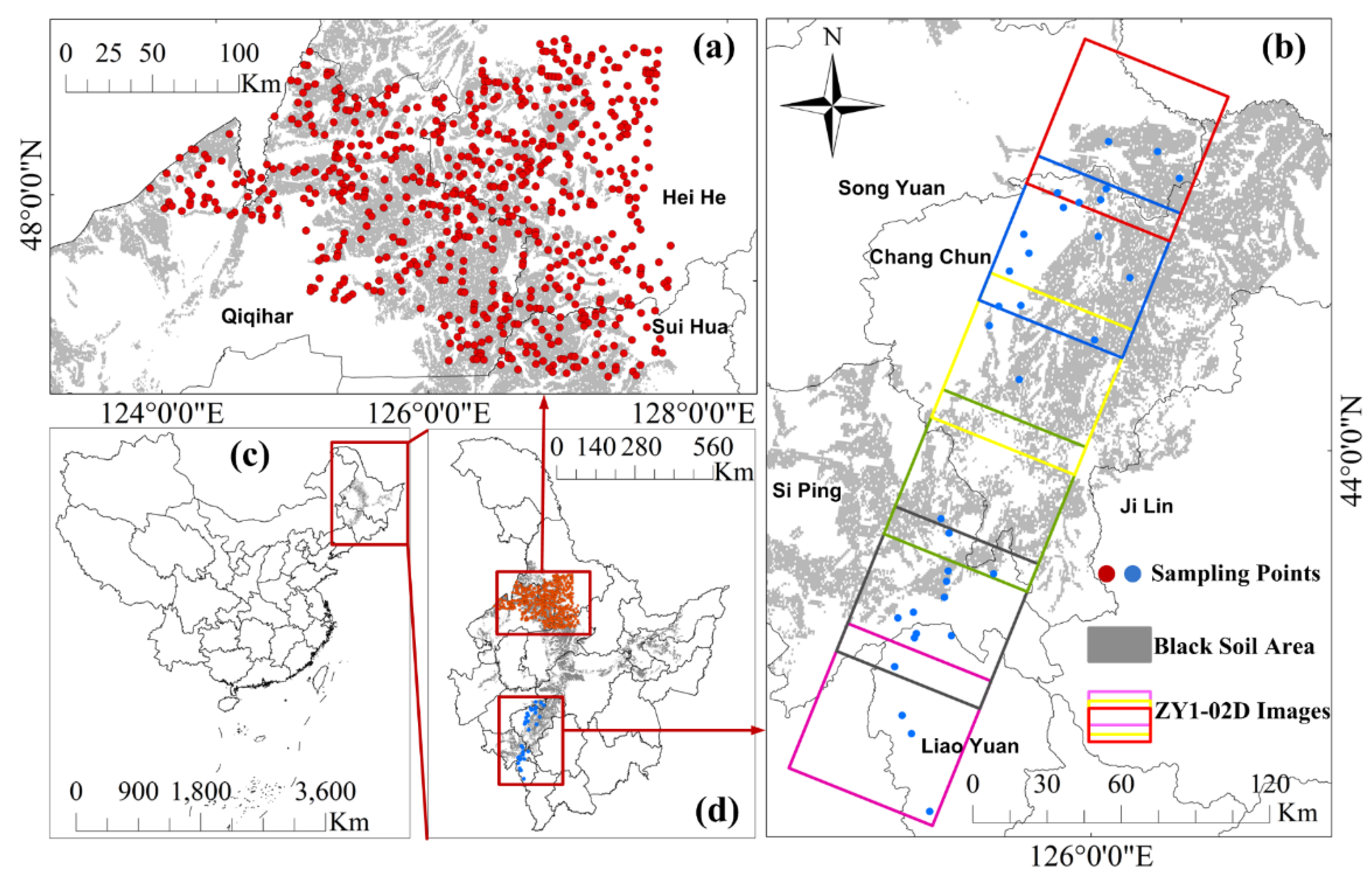
2.1. Study Area

Black soils, also known as Mollisols (USDA) and Chernozems, Kastanozems or Phaeozems (FAO), are widely distributed in the Ukrainian plain, Mississippi Valley, Northeast China and Pampas Steppe, and totally cover about 916 million hectares around the world [1]. The farmlands covered by black soils are recognized as fertile and valuable resources which are widely and intensively explored and farmed in the three regions around the latitude of N46°of the northern hemisphere [1,2], which significantly overlaps with the main maize, soybean and wheat growing regions of the world [3]. The black soils of China are primarily located in three provinces (Liaoning, Jilin and Heilongjiang) in northeast China that cover an area of 124.9 × 10 4 km2 [1]. According to the FAO 90 classification system, the typical black soil (Haplic Phaenozems) region in northeast China could be extracted from the Harmonized World Soil Database and shown as the gray area in Figure 1 [50]. The farmlands cover most of the study area (86%) and the main crop types in the study area are maize, and rice grown in an area located alongside the basin of the Songhua river and its tributaries. Soil samples (n = 646) from the typical black soil fields in northeast China were collected for our spectral and geochemical analysis.

2.2. Data Sets

2.2.1. Sampling and Geochemical Measurement

The majority soil samples for sensitive bands analysis (n = 600) were collected from the typical black soil belt in Heilongjiang Province (47°25′32.68″N to 49°8′51.44″N, 123°41′22.34″E to 127°44′8.53″E) in September 2016 and May 2017. Additionally, 46 soil samples were collected in the typical black soil belt in Jilin Province (42°33′19.51″N to 45°11′4.82″N, 124°55′45.07″E to 126°8′47.57″E) in October 2018. All of the samples have exact coordinates recorded with WGS84 latitude and longitude. Both the spectra measurement and geochemical analysis were performed at the laboratory in Liaoning Research Institute of Geology and Mineral Resources (Shenyang, China). The soil samples were air dried, crushed and sieved through 0.075 mm sieve in the laboratory for spectral measurement and geochemical analysis. The total nitrogen (TN) content was measured by the Kjeldahl distillation volumetric method. To illustrate the variability of the sensitive bands due to the changes of samples, 50 samples were randomly selected from the 600 samples five times for the sensitive bands selection calculation (named as datasets for test, Dt1 to Dt5). Owing to the stable tendency of the sensitive bands with the increase of the sample size, the 600 samples have been divided into five sample sets with 50–100–200–400–600 samples each for sensitive bands selection calculation, each of these 5 data sets were selected with even gradient variation of TN contents of corresponding samples (named as datasets for sensitive bands selection, Ds1 to Ds5). Another dataset with the 46 soil samples for the calibration and validation procedure with ZY1-02D (AHSI) data for the soil N content estimation were named the datasets for estimation (De). Descriptions of the datasets are listed in Table A2.

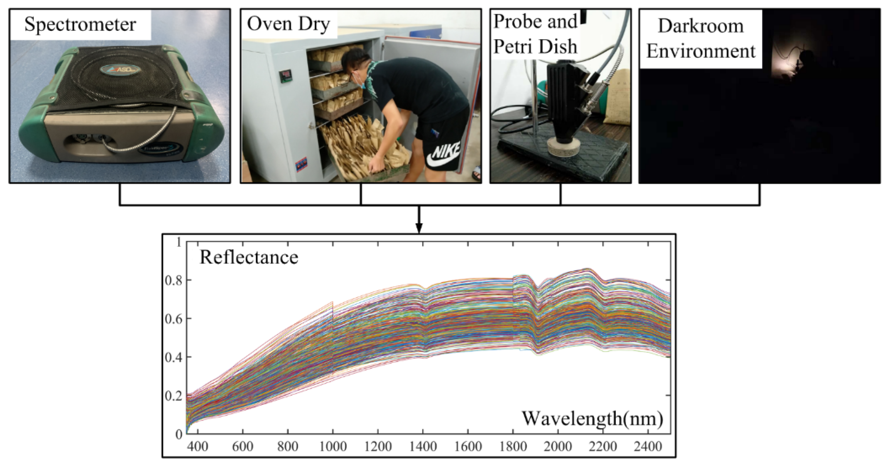
2.2.2. Spectral Measurement

Spectral reflectance data of soil samples were measured by an ASD Fieldspec® 3 spectrometer (ASD Inc., Boulder, CO, USA) with spectral sampling interval of 1 nm, spectral resolution of 3 nm at visible, 8.5 nm at NIR and 6.5 nm at SIWR across a spectral region of 350–2500 nm. The complete set of data were spectrally measured in the lab follow a uniform protocol during the same period and under the constant experiment environment. The dark room condition avoided light interference with the probe light source of the spectrometer; the oven drying process applied to the soil samples before the spectral measurements minimized the moisture effects on the reflectance; during the course of measurement, under the iron supported fixed probe, soil samples were placed in a Petri dish and the surface was flattened for the measurements. The laboratory environment and materials are shown in Figure 2. The spectrometer and the bulb (4.05 W tungsten halogen lamp with 2901 ± 10° %K color temperature) in the probe should be warmed up for half an hour before the measurements are recorded. During measurement course, the standard white reference panel should be measured once per half an hour for spectrometer calibration. Each soil sample was measured five times.

2.2.3. ZY1-02D Hyperspectral Image

We used six ZY1-02D hyperspectral images acquired on the typical black soil belt in Jilin province in 13 May 2020 (Figure 3). The images collected in May covered well the bare soil exposed during the season. May corresponds to the period before the bud burst and after the tillage of farmlands. The ZY1-02D (AHSI) was lunched on 12 September 2019, and has the following characteristics: 166 bands (spectral resolution of 10 nm at VNIR and 20 nm at SWIR), 400 nm to 2500 nm spectral region, swath width of 60 km and the spatial resolution of 30 m [45]. The experimental ZY102D (AHSI) images in this study were provided by the Land Satellite Remote Sensing Application Center.

2.2.4. GlobeLand30 Dataset

The GlobeLand30 land cover dataset (GLC30) is a global scale land cover classification dataset with 30 m spatial resolution. GLC30 (version 2000) and GLC30 (version 2010) were developed and published by the National Geomatics Center of China in 2014 [51,52]. The latest version, GLC30 V2020, which provides an overall classification accuracy of 85.72% (Kappa: 0.82) for ten classes of land cover (http://www.globallandcover.com/ (accessed on 16 October 2021)) was used in this study to extract the farmland region in the study area.

2.3. Data Pre-Processing

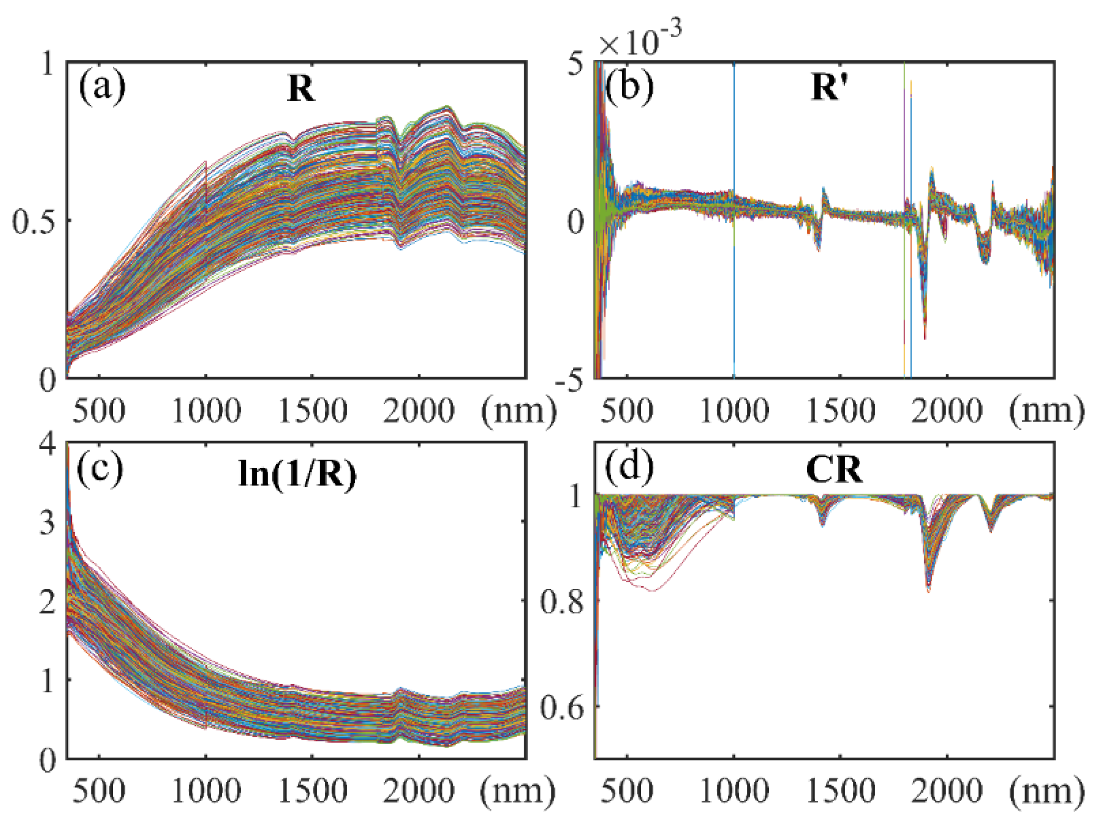
2.3.1. Laboratory Spectra Pre-Processing

The spectral datasets for sensitive bands analysis were generated by the procedure of pre-processing the lab spectra. The raw spectra collected by the spectrometer were reflectance transformed and exported as ASCII files in the ViewSpec Pro software. Spectral smoothing was carried out by applying the Savitzky-Golay algorithm [53]. The average of five repeated observations was calculated to represent the spectral reflectance (R) of each sample. Studies proved that spectral transformation procedure could generally enhance the spectral characteristics and improve the estimation accuracy to the soil properties [54,55,56,57,58,59]. For contrast experiment, three types of spectral transformation were applied in this study: the first derivative of the reflectance (R’), the logarithm of the reciprocal of the reflectance (ln(1/R)) and the continuum removal (C) (Figure 4).

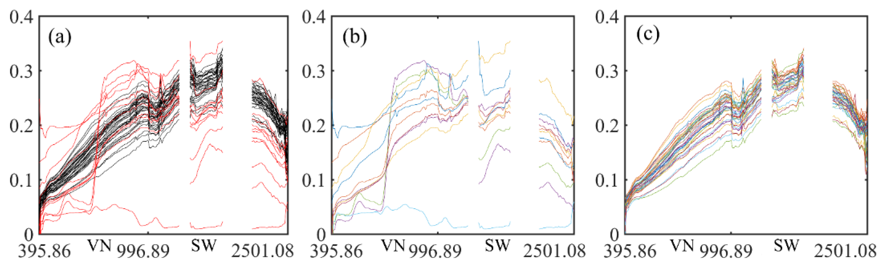
2.3.2. Hyperspectral Image Pre-Processing

The six ZY1-02D (AHSI) images we used in this study are 1A-level products. The geometric correction was carried out with the rational polynomial coefficient model, the radiometric calibration procedure was performed using the linear relationship function, the fast line-of-sight atmospheric analysis of hypercubes (FLAASH) algorithm with the MODTRAN5 radiation transmission model was applied to perform the atmospheric correction and convert the radiance into reflectance. The pre-processing procedures mentioned above were performed in the Environment for Visualising Images (ENVI 5.4, Research Systems, Boulder, CO, USA). The geospatial raster images of the spectral reflectance of ZY1-02D would be derived after pre-processing. The spectral reflectance of the pixels at the position of 46 sampling points within the region of images (the De dataset) were extracted from the processed images as shown in Figure 5a. Spectra that do not have the characteristics of bare soil, as shown in Figure 5a,b, would be removed. The VNIR-SWIR overlapping bands in VNIR spectral region, band72-band76 (1005.8364 nm–1040.2012 nm), as well as the water vapour absorption bands, band97-band102 (1341.1559 nm–1425.3328 nm) and band125–band132 (1812.0157 nm–1929.9292 nm) were not considered in our modelling.
Corresponding to the spectral transformation of the lab spectra, three forms of spectral transformations were also performed to the spectral reflectance obtained from the ZY1-02D images (Figure 6). Results show consistent spectral characteristics with the lab spectra of soil samples (Figure 4), that confirms the good data quality of the ZY1-02D (AHSI) images pre-prepared with the procedure described above.

2.4. Methodology

2.4.1. Sensitive Spectral Algorithm

The Pearson correlation coefficient was applied to estimate the correlation between the soil N content and the spectra value of each band on full VN-SWIR wavelength. We defined the threshold of 0.4 to select the sensitive bands to the soil N content. The correlation coefficient of the datasets Dt1–Dt5 would be calculated and plotted to illustrate the soil N sensitive bands variability, and the correlation coefficient of the datasets Ds1–Ds5 would be calculated and plotted to illustrate the sensitive bands stable tendency.

2.4.2. Partial Least Squares Calibration and Validation

Partial least-squares regression (PLSR) was carried out to establish the relationship between the spectra and soil N content. The full wavelength ZY1-02D spectral reflectance and the spectra of three forms of spectral transformation would be considered as independent variables for PLSR modelling respectively to compare their soil N estimation capabilities. Correspondingly, the obtained sensitive bands of four forms of spectra would be considered as independent variables for PLSR modelling respectively for a comparative analysis.
The PLSR procedure isoften applied for multi-linear regression modelling with high dimensional collinear independent variables modelling such as hyperspectral data [34,35]. We used the SIMPLS algorithm [60] to carry out the PLSR procedure in MATLAB (MathWorks, Inc. Natick, MA, USA). The algorithm projects the independent variables into several orthogonal PLS components as the latent variables (LVs) to reduce the dimensionality of them. The percentage of variance explained in variables by the LVs is defined as the PCTVAR, which is usually applied to support the decision of the number of LVs for modelling [61]. The larger the cumulative value of PCTVAR with the increase of LVs indicates the more the variables are explained by the LVs. Moreover, the lower root mean square error (RMSE) from cross validation is also usually applied to determine the optimal LVs to avoid underfitting or overfitting of PLSR models [62]. Hence, in this study, we define the maximum value of the ratio of PCTVAR and RMSE, the RPR, to determine the optimal number of latent variables for PLSR calibration. The 10-fold cross validation was carried out to calculate the RMSE of validation (RMSEv). On the other hand, both the RMSE of calibration (RMSEc) and the RMSEv were applied to quantify the inaccuracy of the estimates of the models, and the coefficient of determination of calibration and validation (R2c and R2v) was applied to assess the estimation accuracy of the models.

2.4.3. Soil Nitrogen Content Mapping

The optimum model for the soil N content estimation would be derived from the validation procedure. Spectral data required by the optimum model of each pixel of all ZY1-02D images were extracted for nitrogen content estimation calculation by using the optimum model to create geospatial raster data. The farmland region raster data of the GLC30 land cover dataset would be extracted as a mask for the N estimation result clipping. The results would be mapped in the ArcMap 10.2 environment (Esri China Information Technology Co. Ltd., Beijing, China).

3. Results

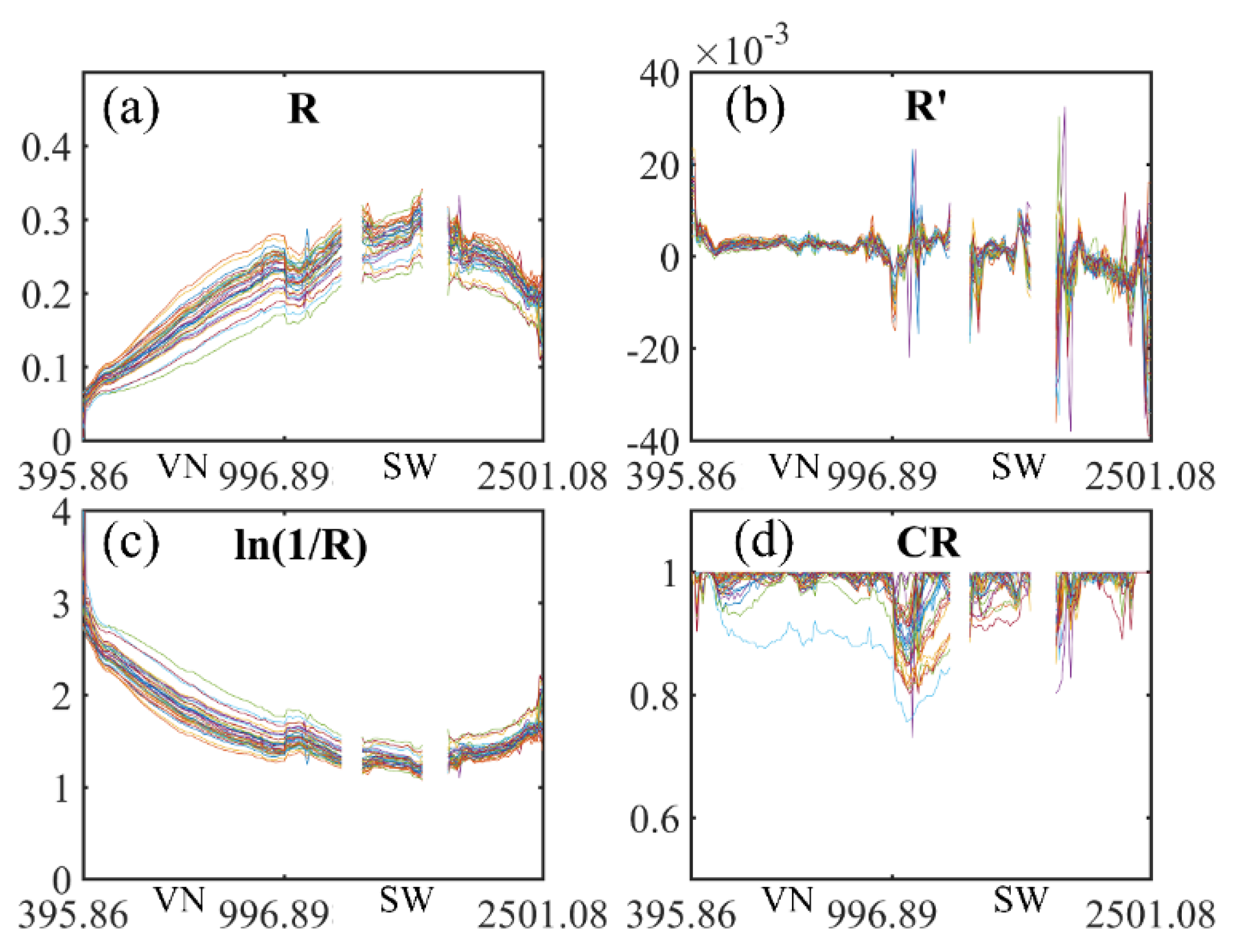
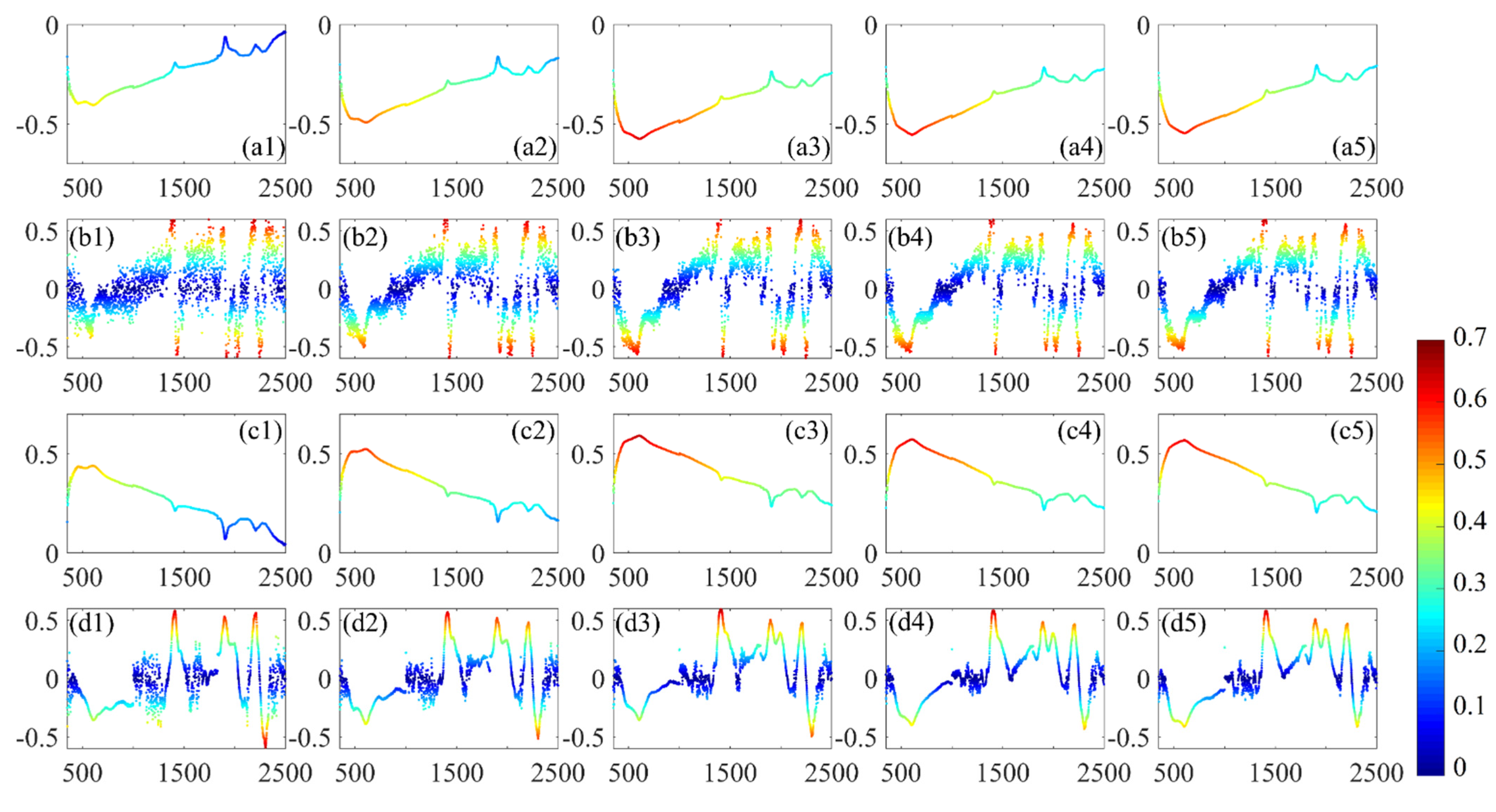
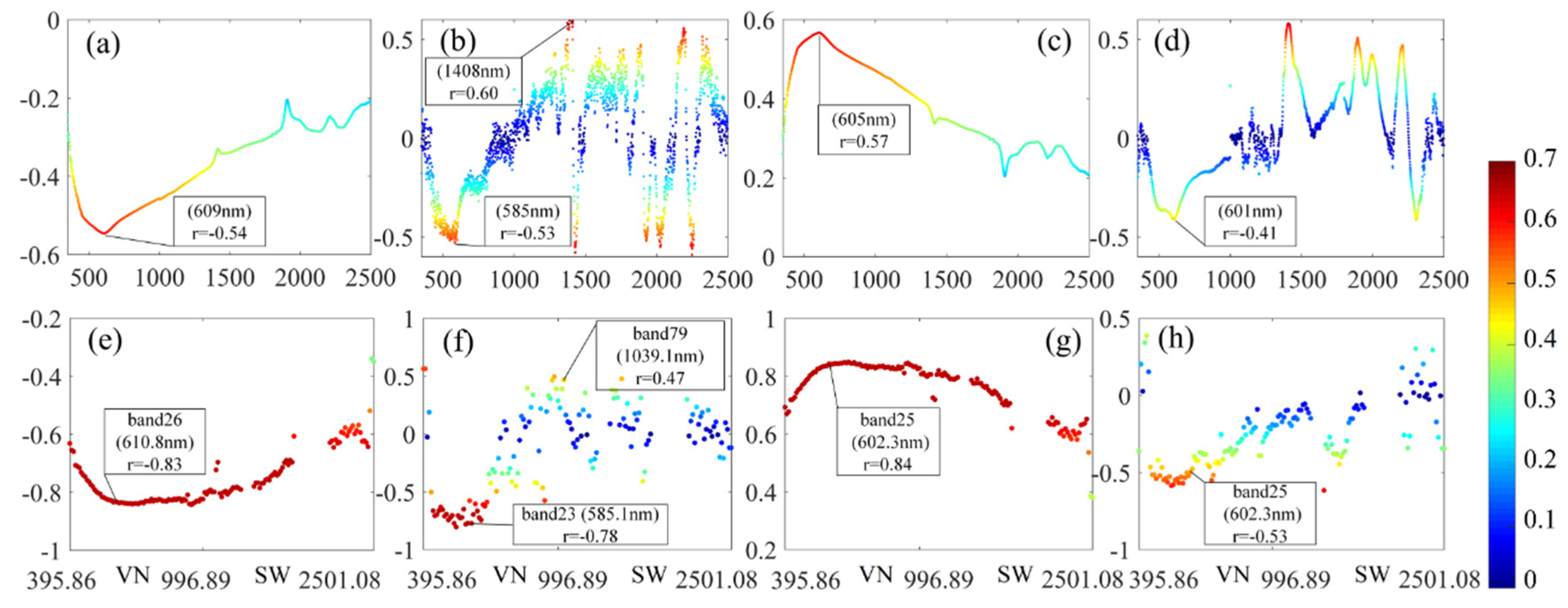
3.1. Sensitive Spectral Bands for Soil N Content Estimation

The correlation coefficient between N content and the spectral reflectance (R) on whole VN-SWIR region of five datasets for test (Dt1 to Dt5) are shown in Figure 7(a1–a5). The results show the obvious variability with the change of the datasets. Correspondingly, the sensitive bands results of the first derivative of the reflectance (R’) of Dt1 to Dt5 are shown in Figure 7(b1–b5). Besides the result variation with the change of the datasets, (b1) to (b5) show an obvious discontinuity of the correlation coefficient on continuous VN-SWIR wavelength. Even though the R’ spectra increased the region of the high correlation bands than the results of R spectra, such discontinuity may lead to a significant variation of the correlation coefficient caused by the slight band anomaly, and then lead to the inaccuracy of the N content estimation modelling based on the sensitive bands. Correspondingly, Figure 7(c1–c5) show the sensitive bands results of the ln(1/R) spectra. These results are almost symmetric about the line axis x with the corresponding results of (a1) to (a5). The last group of (d1) to (d5) show the correlation coefficients between the CR spectra and the N contents of Dt1 to Dt5.
The correlation coefficients between N content and the spectral reflectance (R) on whole VN-SWIR spectral region of five datasets for sensitive bands selection (Ds1 to Ds5) are shown in Figure 8(a1–a5). Correspondingly, the results of the R’, ln(1/R) and CR spectra are shown in Figure 8(b1–d5), respectively. These results show the obvious stable tendency of the correlation coefficient between the spectra and the soil N contents with the increase of the sample size:
(a1)–(a5): for the spectral reflectance, when the number of samples increase from 50 to 600 (Ds1–Ds5), the correlation coefficient between the spectral reflectance and the soil N content tend to be stable on whole VN-SWIR wavelength. The most sensitive band converges to 609 nm (r = −0.54), and a continuous highly correlated range with 876 bands from 385 to 1260 nm (|r| > 0.4) is obtained;
(b1)–(b5): for the R’ spectra, with the increase of the numbers of sample, not only does the correlation coefficient tend to be stable, but also the discontinuity of the correlation coefficient tends to be convergent. Furthermore, the R’ spectra obtained 11 stable soil N content highly correlated range (Table 1);
(c1)–(c5): for the ln(1/R) spectra, the symmetric characteristics against the R results is present again, correspondingly, the most sensitive band converges to 605 nm (r = 0.57), and obtained a continuous highly positive correlated range with 920 bands from 378 to 1297 nm;
(d1)–(d5): for the R’ spectra, the increase of the sample size has also stabilized the change of the correlation coefficient on whole VN-SWIR wavelength. Moreover, the highly correlated ranges are more continuous than the R’ results. Furthermore, six stable soil N content highly correlated rangex are obtained as listed in Table 1.
Through the results of the sensitive spectral bands analysis, we obtained the sensitive bands to the soil N content of the spectral reflectance and the spectra of spectral transformation (Figure 9a–d). In order to verify the universality of these results to the ZY1-02D hyperspectral data, the sensitive bands to the soil N content of the ZY1-02D hyperspectral data based on the datasets for estimation (De) were calculated and plotted in Figure 9e–h:
(a)&(e): As shown in Figure 9e, the correlation coefficient between the spectral reflectance of ZY1-02D and the soil N content performs the consistent tendency comparing with the lab spectra result in Figure 9a, and even obtained higher correlation in VNIR spectral region. For ZY1-02D, band26 is closest to the most sensitive band of lab spectra (609 nm), and it obtained an ideal correlation coefficient of −0.83;
(b)&(f): For the results of the R’ spectra, comparing with the lab spectra result (b), the ZY1-02D spectra result (f) provides a consistent highly correlated range near the optimal sensitive band of 585 nm, the band23 at 585.1 nm achieves an ideal correlation coefficient of −0.78, which is even higher than the lab spectra. The sensitive band of 1408 nm of lab spectra also has obtained an ideal match at band79 (1039.1 nm), which achieves the correlation coefficient of 0.47;
(c)&(g): What is consistent with the result of lab ln(1/R) spectra (c) is the correlation coefficient between the soil N content with the ln(1/R) spectra of ZY1-02D (g) show the same symmetric characteristics against the R spectra results (e). Furthermore, the high correlated range near the band25 (602.3 nm) is consistent with the sensitive range of the lab spectra.
(d)&(h): For the results of the CR spectra, although the sensitive bands of lab spectra in the SWIR spectral region (d) are not well represented in the result of ZY1-02D spectra (h), the sensitive bands of ZY1-02D mainly converged to the VNIR spectral region near the band25 (602.3 nm) that matches consistently with the results of the lab CR spectra;

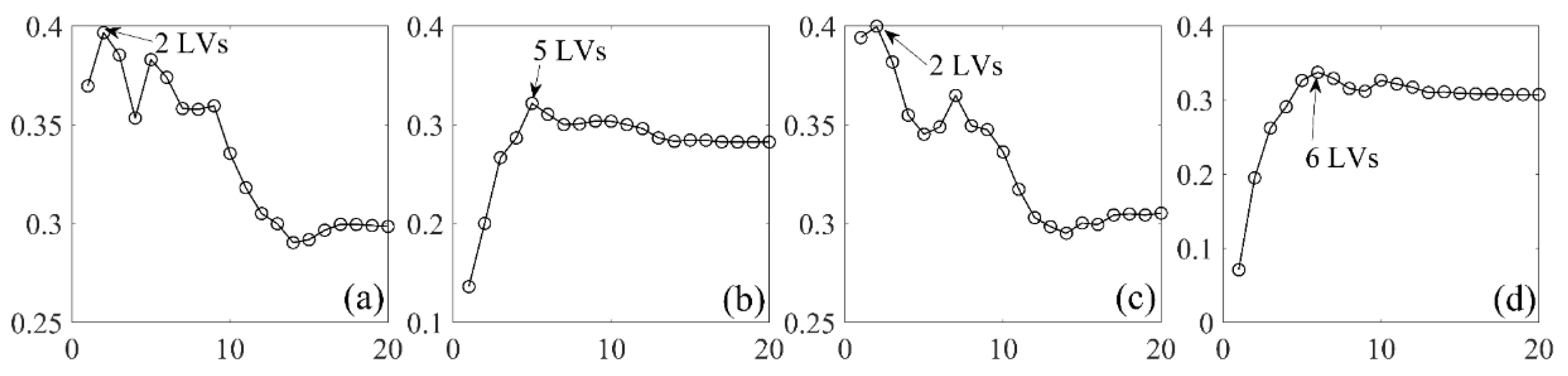
3.2. PLSR Calibration and Validation for Soil N Content Estimation

As shown in Figure 10a, the PLS model developed with the spectral reflectance achieved the maximum RPR value when two latent variables (LVs) were considered as the optimal number of LVs for modelling. Correspondingly, the 5, 2 and 6 LVs were considered as the optimal number of the LVs for PLS modelling for the models developed with the spectra of R’, ln(1/R) and CR respectively (Figure 10b–d).
For the models derived from the same spectral form, the same number of LVs were employed for modelling to keep the spectral region as the unique variable for comparative analysis. Figure 11 and Table 2 presents the results of estimation accuracy of the models in calibration and validation. The model developed with the R’ and CR spectra have all achieved ideal calibration accuracy, and particularly, the model developed with the full wavelength CR spectra that used 6 LVs achieved the optimum calibration result (R2c = 0.90 and RMSEc = 96.68). However, they all presented poor estimation accuracy in validation, which partly due to the relatively poor correlation between the soil N content and the spectra on whole VN-SWIR region (Figure 9). In contrast, the models developed with the R and ln(1/R) spectra achieved ideal estimation accuracy in validation, especially, the model developed with the sensitive bands of original spectral reflectance that used only two LVs achieved the optimum validation result (R2v = 0.66 and RMSEv = 175.74), which partly due to the relatively high and continuous correlation between the soil N content and the spectra on whole VN-SWIR region (Figure 9).
As is shown in results that the calibration accuracy would be enhanced with the increase of the LVs. However, the more LVs always presented low validation accuracies on account of the overfitting risk due to the increase of the PLS components [43,63,64]. It is noteworthy that models developed with the sensitive bands even achieved better validation accuracy than the full wavelength spectra models. That proves that the sensitive bands modelling could enhance the accuracy of the estimation, furthermore, could reduce the number of independent variables and then simplify model.

3.3. Soil N Contents Estimaiton and Mapping

The main result of the estimation is a geospatial raster map with 30 m spatial resolution that shows the spatial distribution of the topsoil total N content of the farmlands in the Jilin black soil belt in northeast China. The 92,384 abnormal pixels with negative value of the geospatial raster map were removed to refine the result. The refined raster was clipped by the mask of the GLC30 data to remove the regions outside the farmlands. Total 18,705,319 pixels were considered as the effective values to determine the lower and upper boundary (568.94 and 2380.81) of the estimation refer to the 95% confidence interval. The final mapping result is shown in Figure 12. The total N content in topsoil varied significantly among the study area, ranging from 568.94 to 2380.81 μg/g with an obviously higher in central area, the Changchun region, which significantly overlaps the typical black soil area.

4. Discussions

The results in Figure 7 show that when the sample size is small, no matter what kind of spectral transformation was performed, the correlation between the spectra and soil N content would differ significantly with the change of samples. This result is consistent with previous reports [65]. Furthermore, the results shown in Figure 8 demonstrate that the sensitive spectral bands to the soil N content on the whole VN-SWIR spectral region would tend to be stable with the increase of the sample size, and the sensitive bands would be convergent to one or more certain specific regions: the R and ln(1/R) spectra on whole VN-SWIR spectral region achieved a stable continuous high correlation with the soil N content, and conversely, the results of the R’ and CR spectra show an obvious discontinuity in the whole VN-SWIR spectral region, which is consistent with the previous reports [66,67]. These results have shown the effective behavior of the model calibration validation result: the stable and consistent sensitive region would produce very stable estimation results, that the model developed with R or ln(1/R) spectra in most of statistics reached a higher R2 and lower RMSE (Table 2). This result is consistent with what previous studies have reported [26,68]. However, the model developed with R’ or CR spectra obtained poor estimation accuracies, which is also consistent with previous reports [67,68]. Development of estimation models of soil properties based on proximal and remote sensing spectral data for large spatial scale mapping is a complex procedure [65]. Previous studies demonstrated that the accuracy of soil property estimation by using spectral analysis methods would be influenced by many factors [16,31,44]. Among them, the sample size plays an important role in affecting the accuracy of the estimation. Our study has demonstrated this influence by analyzing the sensitive spectral bands to the soil N content and consequently observing the variability upon changing the sample sets.
Furthermore, the sensitive bands of the lab spectra show ideal universality with the ZY1-02D hyperspectral data as shown in Figure 9. This result not only demonstrates the ideal data quality of the ZY1-02D (AHSI) data, but also provides a theoretical basis for further studies to employ the conclusions based on the lab spectra to the spaceborne ZY1-02D (AHSI) data. Previous studies usually used data of all bands for modelling to enrich the number of independent variables when multispectral images were applied as the data source. Even so, they could hardly achieve the estimation accuracy seen in our study: the R2 of 0.49 of Landsat 5TM [38], 0.44 of Sentinel-1A [40], 0.37 and 0.51 of Landsat 8 OLI [40,41], 0.32 and 0.46 of Sentinel-2A [39]. Gopal et al. and Vilem et al. applied Hyperion and CASI-SASI hyperspectral images for soil N content estimation modelling respectively [37,38]. They used full wavelength spectra for PLSR modelling and achieved accuracies of R2 = 0.63 and R2 = 0.44 respectively, which are lower than those of our study. Anne et al. used the sensitive bands of Hyperion for soil N content estimation PLSR modelling and achieved the ideal accuracy of R2 = 0.69, which was higher than the estimation accuracy of our study. The sensitive bands of 530 nm-590 nm and 700–790 nm are within the range of the sensitive bands of our study [36]. Results show that the ZY1-02D (AHSI) could achieve the ideal, and even better accuracy for soil N content estimation comparing with other spaceborne or airborne hyperspectral imagers.
The result of topsoil N content estimation and mapping in our study accurately detected the spatial soil N content distribution feature in the black soil area of Jilin Province (China), which is consistent with the previous records [69,70]. The region in Songyuan shows an obvious lower soil N content mainly due to the fairly severe soil N leaching process of the Acrisols existing in this region [71]. The southern region shows a contrasting result with the previous study, in that the soil N content was underestimated in this study [70]. This is probably because of the abnormal spectra caused by the uncertainty of the land covers [16,31,44]. Most parts of this region are covered by paddy fields [72], whose spectral reflectance would generally reduce with the increase of the soil moisture on account of the effect of the irrigation in May, which consequently resulted in a decrease in the estimation [73].
Overall, the model developed with the sensitive bands of the spectral reflectance could be regarded as the optimum model for soil N content estimation in this study. Moreover, its succinct modelling procedure that carried out with the several certain bands of the original spectral reflectance data should be easier to perform in any further studies. Furthermore, the results of this study demonstrated the good capacity of ZY1-02D (AHSI) in soil N content estimation. It also demonstrates a good potential of this hyperspectral imager in detecting more information. In future studies, more important properties such as SOC, heavy metal levels, soil moisture, etc. of soil should be investigated using this hyperspectral data.

5. Conclusions

This study demonstrated that the ZY1-02D (AHSI) showed an ideal capability for topsoil nitrogen content estimation and mapping at the regional scale. The experiments of this study achieved several ideal results, which allow the following conclusions to be drawn:
Firstly, in the sensitive spectral band analysis experiment of our study, we found and demonstrated the variability and stable tendency of the sensitive spectral bands to the soil N content with the change of the sample size: The sensitive spectral bands to the soil N content in the whole VN-SWIR spectral region showed significant variability with the change of the datasets when the sample size was small. Nevertheless, the sensitive spectral bands to the soil N content on whole VN-SWIR spectral region would tend to be stable with the increase of the sample size, and the sensitive bands would converge to one or more certain specific regions. On the one hand, this result provided a theoretical support for selecting the sensitive spectral bands to estimate soil N content and subsequent analysis to this study. On the other hand, it also provides an effective method for selecting sensitive bands for the estimation of other soil properties, moreover, improving the estimation accuracies.
Secondly, the sensitive bands derived from the proximal lab hyperspectral data showed ideal consistency with the sensitive bands derived from the ZY1-02D (AHSI) remote sensing data. This demonstrates the good data quality of the ZY1-02D (AHSI) hyperspectral data, moreover, it provides a theoretical basis for the application of the results of the spectral analysis with the lab spectra to the spaceborne ZY1-02D (AHSI) data. In this study, the sensitive bands to the soil N content of the spectral reflectance and its four forms of spectral transformation to the black soil N contents were presented, which could be applied as a reference in the future studies.
Thirdly, the PLSR models developed with the sensitive bands of spectra would achieve a better estimation accuracy than the models developed with the full wavelength spectra. The replacemwnt of the full wavelength spectra by the sensitive spectra could not only enhance the estimation accuracy, but also could help simplify the models.
Finally, the PLSR models developed with the sensitive bands of the spectral reflectance of the ZY1-02D (AHSI) obtained an optimum validation accuracy (R = 0.66), demonstrating that the ZY1-02D (AHSI) could achieve ideal, and even better accuracy for soil N content estimation comparing with other spaceborne or airborne hyperspectral image sources (Hyperion and CASI-SASI).
Despite the ideal estimation accuracy obtained in the black soil area on a regional scale by the current work, there is still room for the further research to improve the results, especially in the further validation of the model in time series applications. If the model can obtain good estimation accuracy in multi-temporal ZY1-02D (ASHI) data, then one could realize a long time series monitoring program of the change of the soil N content in the black soil region. Further work will also be focused on the contrastive analysis with more types of algorithms for sensitive bands analysis and modelling. Moreover, the potential of the ZY1-02D (ASHI) for the estimation of more soil attributes such as the soil organic carbon content, the soil heavy metal content and soil moisture content, etc. could be investigated in the further studies.

Author Contributions

Conceptualization, Z.X. and S.C.; Methodology, Z.X.; Software, Z.X., B.Z. and L.C.; Validation, Z.X. and S.C.; Formal Analysis, Z.X.; Investigation, Z.X., Y.Y. and B.Z.; Resources, S.C. and P.L.; Data Curation, Z.X. and S.C.; Writing-Original Draft Preparation, Z.X.; Writing-Review & Editing, Z.X.; Visualization, Z.X.; Supervision, S.C.; Project Administration, S.C. and P.L.; Funding Acquisition, S.C. and P.L. All authors have read and agreed to the published version of the manuscript.

Funding

This research was supported by National Key Research and Development Program of China (No. 2020YFA0714103), Jilin Province Science and technology development plan (20210201138GX), Jilin Province Science and technology development plan (20210203016SF), the Land Resource Evolution Mechanism and Its Sustainable Use in Global Black Soil Critical Zone (IGCP665) funded by IUGS and UNESCO.

Institutional Review Board Statement

Not applicable.

Informed Consent Statement

Not applicable.

Data Availability Statement

Not applicable.

Acknowledgments

The experimental ZY102D (AHSI) images in this study were provided by the Land Satellite Remote Sensing Application Center, China. The soil samples with the geochemical analysis data were provided by Shenyang Geological Survey of China Geological Survey, China. Both the spectra measurement and geochemical analysis were performed at the laboratory in the laboratory in Liaoning Research Institute of Geology and Mineral Resources, China, which provide the experimental sites and materials. Part of the spectral measurement work was supported by the College of Surveying and Exploration Engineering, Jilin Jianzhu University, Changchun, China.

Conflicts of Interest

We declare that we do not have any commercial or associative interest representing a conflict of interest in connection with the submitted manuscript.

Appendix A

Table A1. A review of the studies comparing quantitative analysis of soil N content using calibration and validation modelling method by the ground spectra and remote sensing data.
YearAttributeDataMethod aModelling Bands(nm)Cal/Val bR2Author
1986N (total); %LabMLR1702, 1870, 205272/480.92Dalal et al.,
1999N (total); mg/kgLabPLSR1100–2498120/590.95Reeves et al.,
2001N (total); g/kgLabPCR400–249830/1190.85Chang et al.,
2002N (total); g/kgLabPLSR400–249876/320.86Chang et al.,
2003N (total); g/kgLabPLSR400–2500144/cross0.62Thomas et al.,
2004N (total); g/kgLabPLSR400–2500174/cross0.95Moron et al.,
2007N (total); mg/gLabPLSR350–2500103/cross0.87Mutuo et al.,
2011N (total); g/kgLabPLSR1250–2500217/780.95Xie et al.,
2013N (total); g/kgLabSMLR1400, 225096/cross0.48Shi et al.,
2013N (total); g/kgLabPLSR1450, 1850, 2250, 2330, 243096/cross0.56Shi et al.,
2013N (total); g/kgLabSVM350–250096/cross0.58Shi et al.,
2017N (total); g/kgLabPLSR900–1700118/580.79Xiao et al.,
2019N (total); %LabPLSR900–1700100/500.92Li et al.,
2019N (total); %LabPLSRUVE c100/500.93Li et al.,
2019N (total); %LabPLSRSPA c100/500.92Li et al.,
2014Stable N; mg /gHyperionPLSR530–590; 700–790; 1500–1590; 2200–233018/NaN0.69Anne et al.,
2015N (total); g/kgHyperionPLSR155 bands78/300.63Gopal et al.,
2018STN; g/kgLandsat 5 TMSMLRRGB + NDVI92/230.49Wang et al.,
2019N (total); g/kgSentinel-2ARF13 bands104/cross0.32Zhang et al.,
2019N (total); g/kgSentinel-2ARF12 Indices104/cross0.46Zhang et al.,
2019N (total); g/kgLandsat 8 OLIBRT/RF/SVMRGB + NDVI85/cross0.37Zhou et al.,
2019N (total); g/kgSentinel-1ABRT/RF/SVMBackscatter coefficients85/cross0.44Zhou et al.,
2020N (total); kg m−2Landsat 8 OLIGWR/MLSR/BRT12 Indices410/1030.51Wang et al.,
2020STN; g/kgSentinel-1A + Sentinel-1B + Sentinel-2ABRT/RF/SVMBackscatter coefficients + RGB + 3 indices179/cross0.21Zhou et al.,
2021N (total); %Airborne(CASI-SASI)PLSR380–245022/cross0.44Vilém et al.,
a Calibration methods include multiple linear regression (MLR), partial least squares regression (PLSR), principle component regression (PCR), stepwise multiple linear regression (SMLR), boosted regression trees (BRTs), random forest (RF), and support vector machine (SVM), geographical weighted regression (GWR). b Cal/Val indicate the number of samples that applied in the calibration and validation procedure. Cross suggests that in the validation procedure, the cross validation was used, and NaN indicates that there was no validation procedure in the corresponding study. c Some studies have employed the sensitive band selection method as the uninformative variable elimination (UVE) and the successive projections algorithm (SPA).
Table A2. Datasets for this research.
Data
Sets
Sample
Size
Nitrogen Content (μg/g)SDVC
MinQ1MedianQ3MaxMean
Dt150132920702366280042062500.40696.150.278
Dt250143320342398281339302511.58565.060.225
Dt350129219912329265734142333.00500.780.215
Dt450137220012203246230132234.16380.330.170
Dt550125616742138236528012084.64435.820.209
Ds150122419502335.5295046952550.80817.560.321
Ds2100122419822343.5307347982568.92823.380.321
Ds3200122419912354307650312579.28829.080.321
Ds4400122423522356235652272583.28832.130.322
Ds5600122419962356308952692586.63834.260.323
De4678111711365153623341393335.750.24
Q1 indicates the first quartile, Q3 indicates the third quartile, SD indicates the standard deviation, and VC indicates the variation coefficient.

References

  1. Liu, X.; Burras, C.L.; Kravchenko, Y.S.; Duran, A.; Huffman, T.; Morras, H.; Studdert, G.; Zhang, X.; Cruse, R.M.; Yuan, X. Overview of mollisols in the world: Distribution, land use and management. Can. J. Agric. Sci. 2012, 92, 383–402. [Google Scholar] [CrossRef]
  2. Zhang, Z.; Sui, Y. A Brief Introduction to Chinese Mollisols, New Advances in Research and Management of World Mollisols, Harbin, China; Liu, X.B., Song, C.Y., Cruse, R.M., Huffman, T., Eds.; Northeast Forestry University Press: Harbin, China, 2010. [Google Scholar]
  3. Monfreda, C.; Ramankutty, N.; Foley, J.A. Farming the planet: 2. Geographic distribution of crop areas, yields, physiological types, and net primary production in the year 2000. Global Biogeochem. Cycles 2008, 22, GB1022. [Google Scholar] [CrossRef]
  4. Ajami, M.; Heidari, A.; Khormali, F.; Gorji, M.; Ayoubi, S. Environmental factors controlling soil organic carbon storage in loess soils of a subhumid region, northern Iran. Geoderma 2016, 281, 1–10. [Google Scholar] [CrossRef]
  5. Zhao, Y.; Wang, M.; Hu, S.; Zhang, X.; Ouyang, Z.; Zhang, G.; Huang, B.; Zhao, S.; Wu, J.; Xie, D. Economics– and policy–driven organic carbon input enhancement dominates soil organic carbon accumulation in Chinese croplands. Proc. Natl. Acad. Sci. USA 2018, 115, 4045–4050. [Google Scholar] [CrossRef] [PubMed] [Green Version]
  6. Tilman, D.; Balzer, C.; Hill, J.; Befort, B.L. Global food demand and the sustainable intensification of agriculture. Proc. Natl. Acad. Sci. USA 2011, 108, 20260–20264. [Google Scholar] [CrossRef] [Green Version]
  7. Lu, Y.; Chadwick, D.; Norse, D.; Powlson, D.; Shi, W. Sustainable intensification of china’s agriculture: The key role of nutrient management and climate change mitigation and adaptation. Agric. Ecosyst. Environ. 2015, 209, 1–4. [Google Scholar] [CrossRef]
  8. Zhang, Y.; Sun, C.; Chen, Z.; Zhang, G.; Chen, L.; Wu, Z. Stoichiometric analyses of soil nutrients and enzymes in a Cambisol soil treated with inorganic fertilizers or manures for 26 years. Geoderma 2019, 353, 382–390. [Google Scholar] [CrossRef]
  9. Zhang, F.; Niu, J.; Zhang, W.; Chen, X.; Li, C.; Yuan, L.; Xie, J. Potassium nutrition of crops under varied regimes of nitrogen supply. Plant Soil 2010, 335, 21–34. [Google Scholar] [CrossRef]
  10. Chen, X.; Cui, Z.; Fan, M.; Vitousek, P.; Zhao, M.; Ma, W.; Wang, Z.; Zhang, W.; Yan, X.; Yang, J. Producing more grain with lower environmental costs. Nature 2014, 514, 486–489. [Google Scholar] [CrossRef]
  11. United States Environmental Protection Agency Reactive Nitrogen in the United States: An Analysis of Inputs, Flows, Consequences and Management Options. A Report of the EPA Science Advisory Board. Available online: https://nepis.epa.gov/Exe/ (accessed on 12 August 2021).
  12. Kral, F.; Corstanje, R.; White, J.R.; Veronesi, F. A geostatistical analysis of soil properties in the Davis pond Mississippi freshwater diversion. Soil Sci. Soc. Am. J. 2012, 76, 1107–1118. [Google Scholar] [CrossRef]
  13. Tomer, M.D.; James, D.E.; Schipper, L.A.; Wills, S.A. Use of the USDA national cooperative soil survey soil characterization data to detect soil change: A cautionary tale. Soil Sci. Soc. Am. J. 2017, 81, 1463–1474. [Google Scholar] [CrossRef] [Green Version]
  14. Seaton, F.; Barrett, G.; Burden, A.; Creer, S.; Fitos, E.; Garbutt, A.; Griffiths, R.; Henrys, P.; Jones, D.; Keenan, P.; et al. Soil health cluster analysis based on national monitoring of soil indicators. Eur. J. Soil Sci. 2020, 72, 2414–2429. [Google Scholar] [CrossRef] [Green Version]
  15. Price, J.C. An approach for analysis of reflectance spectra. Remote Sens. Environ. 1998, 64, 316–330. [Google Scholar] [CrossRef]
  16. Ben-Dor, E. Quantitative remote sensing of soil properties. Adv. Agron. 2002, 75, 173–244. [Google Scholar] [CrossRef]
  17. Bengera, I.; Norris, K.H. Determination of moisture content in soybeans by direct spectrophotometry. Isr. J. Agric. Res. 1968, 18, 124–132. [Google Scholar]
  18. Ben-Dor, E.; Banin, A. Visible and near–infrared (0.4–1.1 gM) analysis of arid and semiarid soils. Remote Sens. Environ. 1994, 48, 261–274. [Google Scholar] [CrossRef]
  19. Chang, C.; Laird, D.A.; Mausbach, M.J.; Hurburgh, C.R. Near infrared reflectance spectroscopy–principal components regression analyses of soil properties. Soil Sci. Soc. Am. J. 2001, 65, 480–490. [Google Scholar] [CrossRef] [Green Version]
  20. Daniel, K.W.; Tripathi, N.K.; Honda, K. Artificial neural network analysis of laboratory and in situ spectra for the estimation of macronutrients in soils of Lop Buri (Thailand). Aust. J. Soil Res. 2003, 41, 47–59. [Google Scholar] [CrossRef]
  21. Rossel, R.A.V.; Behrens, T. Using data mining to model and interpret soil diffuse reflectance spectra. Geoderma 2010, 158, 46–54. [Google Scholar] [CrossRef]
  22. Sequeira, C.H.; Wills, S.A.; Grunwald, S.; Ferguson, R.R.; Benham, E.C.; West, L.T. Development and Update Process of VNIR–Based Models Built to Predict Soil Organic Carbon. Soil Sci. Soc. Am. J. 2014, 78, 903–913. [Google Scholar] [CrossRef] [Green Version]
  23. Liu, L.; Min, J.; Manfred, B. Combining partial least squares and the gradient–boosting method for soil property retrieval using visible near–infrared shortwave infrared spectra. Remote Sens. 2017, 9, 1299. [Google Scholar] [CrossRef] [Green Version]
  24. Dalal, R.C.; Henry, R.J. Simultaneous determination of moisture, organic carbon and total nitrogen by near infrared reflectance spectrophotometry. Soil Sci. Soc. Am. J. 1986, 50, 120–123. [Google Scholar] [CrossRef]
  25. Reeves III, J.B.; McCarty, G.W.; Meisinger, J.J. Near infrared reflectance spectroscopy for the analysis of agricultural soils. J. Near Infrared Spectrosc. 1999, 7, 179–193. [Google Scholar] [CrossRef]
  26. Chang, C.; Laird, D.A. Near–infrared reflectance spectroscopic analysis of soil C and N. Soil Sci. 2002, 167, 110–116. [Google Scholar] [CrossRef]
  27. Thomas, U.; Christoph, E.; Thomas, J. Quantitative analysis of soil chemical properties with diffuse reflectance spectrometry and partial least square regression: A feasibility study. Plant Soil. 2003, 251, 319–329. [Google Scholar] [CrossRef]
  28. Moron, A.; Cozzolino, D. Determination of potentially mineralizable nitrogen and nitrogen in particulate organic matter fractions in soil by visible and near-infrared reflectance spectroscopy. J Agric Sci. 2005, 142, 335–343. [Google Scholar] [CrossRef]
  29. Mutuo, P.K.; Shepherd, K.D.; Albrecht, A.; Cadisch, G. Prediction of carbon mineralization rates from different soil physical fractions using diffuse reflectance spectroscopy. Soil Biol. Biochem. 2007, 38, 1658–1664. [Google Scholar] [CrossRef]
  30. Xie, H.; Yang, X.; Drury, C.; Yang, J.; Zhang, X. Predicting soil organic carbon and total nitrogen using mid– and near–infrared spectra for Brookston clay loam soil in Southwestern Ontario, Canada. Can. J. Soil Sci. 2011, 91, 53–63. [Google Scholar] [CrossRef]
  31. Shi, T.; Cui, L.; Wang, J.; Fei, T.; Chen, Y.; Wu, G. Comparison of multivariate methods for estimating soil total nitrogen with visible/near–infrared spectroscopy. Plant Soil 2013, 366, 363–375. [Google Scholar] [CrossRef]
  32. Xiao, S.; He, Y.; Dong, T.; Nie, P. Spectral analysis and sensitive waveband determination based on nitrogen detection of different soil types using near infrared sensors. Sensors 2018, 18, 523. [Google Scholar] [CrossRef] [Green Version]
  33. Li, H.; Jia, S.; Le, Z. Quantitative analysis of soil total nitrogen using hyperspectral imaging technology with extreme learning machine. Sensors 2019, 19, 4355. [Google Scholar] [CrossRef] [PubMed] [Green Version]
  34. Wold, S.; Sjöström, M.; Eriksson, L. PLS–Regression: A Basic Tool of Chemometrics. Chemom. Intell. Lab. Syst. 2001, 58, 109–130. [Google Scholar] [CrossRef]
  35. Rossel, R.; Walvoort, D.; Mcbratney, A.B.; Janik, L.J.; Skjemstad, J.O. Visible, near infrared, mid infrared or combined diffuse reflectance spectroscopy for simultaneous assessment of various soil properties. Geoderma 2006, 131, 59–75. [Google Scholar] [CrossRef]
  36. Anne, N.; Abd-Elrahman, A.H.; Lewis, D.B.; Hewitt, N.A. Modelling soil parameters using hyperspectral image reflectance in subtropical coastal wetlands. Int. J. Appl. Earth Obs. 2014, 33, 47–56. [Google Scholar] [CrossRef]
  37. Gopal, B.; Shetty, A.; Ramya, B.J. Prediction of the presence of topsoil nitrogen from space borne hyperspectral data. Geocarto Int. 2015, 30, 82–92. [Google Scholar] [CrossRef]
  38. Wang, S.; Jin, X.; Adhikari, K.; Li, W.; Yu, M.; Bian, Z. Mapping total soil nitrogen from a site in northeastern china. Catena 2018, 166, 134–146. [Google Scholar] [CrossRef]
  39. Zhang, Y.; Sui, B.; Shen, H.; Ouyang, L. Mapping stocks of soil total nitrogen using remote sensing data: A comparison of random forest models with different predictors. Comput. Electron. Agr. 2019, 160, 23–30. [Google Scholar] [CrossRef]
  40. Zhou, T.; Geng, Y.; Chen, J.; Sun, C.; Lausch, A. Mapping of soil total nitrogen content in the middle reaches of the Heihe river basin in China using multi source remote sensing derived variables. Remote Sens. 2019, 11, 2934. [Google Scholar] [CrossRef] [Green Version]
  41. Wang, S.; Zhuang, Q.; Jin, X.; Yang, Z.; Liu, H. Predicting soil organic carbon and soil nitrogen stocks in topsoil of forest ecosystems in northeastern china using remote sensing data. Remote Sens. 2020, 12, 1115. [Google Scholar] [CrossRef] [Green Version]
  42. Zhou, T.; Geng, Y.; Chen, J.; Pan, J.; Haase, D.; Lausch, A. High-resolution digital mapping of soil organic carbon and soil total nitrogen using DEM derivatives, Sentinel-1 and Sentinel-2 data based on machine learning algorithms. Sci. Total Environ. 2020, 729, 138244. [Google Scholar] [CrossRef]
  43. Pechanec, V.; Mráz, A.; Rozkošný, L.; Vyvlečka, P. Usage of airborne hyperspectral imaging data for identifying spatial variability of soil nitrogen content. ISPRS Int. J. Geo-Inf. 2021, 10, 355. [Google Scholar] [CrossRef]
  44. Mulder, V.; De Bruin, S.; Schaepman, M.; Mayr, T. The use of remote sensing in soil and terrain mapping—A review. Geoderma 2011, 162, 1–19. [Google Scholar] [CrossRef]
  45. Liu, Y.; Sun, D.; Liang, J.; Zhu, H.; Liu, S.; Li, X. Overview of ZY-1-02D Satellite AHSI On-orbit Performance and Stability. Spacecraft Eng. 2020, 29, 93–97. (In Chinese) [Google Scholar]
  46. Bellon-Maurel, V.E.; McBratney, A. Near–infrared (NIR) and mid–infrared (MIR) spectroscopic techniques for assessing the amount of carbon stock in soils e critical review and research perspectives. Soil Biol. Biochem. 2011, 43, 1398–1410. [Google Scholar] [CrossRef]
  47. Demattê, J.A.M.; Bellinaso, H.; Araújo, S.R.; Rizzo, R.; Souza, A.B. Spectral regionalization of tropical soils in the estimation of soil attributes. Rev. Ciênc. Agron. 2016, 47, 589–598. [Google Scholar] [CrossRef]
  48. Moura–Bueno, J.M.; Dalmolin, R.S.D.; Caten, A.T.; Dotto, A.C.; José, A.M.D. Stratification of a local vis–nir–swir spectral library by homogeneity criteria yields more accurate soil organic carbon predictions. Geoderma 2019, 337, 565–581. [Google Scholar] [CrossRef]
  49. Xu, Z.; Chen, S.; Zhang, H.; Song, K. Black soils classification by ground spectral process and analysis. Acta Geol. Sin. (Engl. Ed.) 2019, 93, 152–157. [Google Scholar] [CrossRef] [Green Version]
  50. Food Agriculture Organization of the United Nations/IIASA/ISRIC/ISS–CAS/JRC: Harmonized World Soil Database (Version 1.2). Available online: https://www.fao.org/soils-portal/data-hub/soil-maps-and-databases/harmonized-world-soil-database-v12/en/ (accessed on 6 November 2020).
  51. Chen, J.; Ban, Y.; Li, S. China: Open access to Earth land–cover map. Nature 2014, 514, 434. [Google Scholar] [CrossRef] [Green Version]
  52. Chen, J.; Chen, J.; Liao, A.; Cao, X.; Chen, L.; Chen, X.; He, C.; Han, G.; Peng, S.; Lu, M. Global land cover mapping at 30 m resolution: A POK–based operational approach. ISPRS J. Photogramm. Remote Sens. 2015, 103, 7–27. [Google Scholar] [CrossRef] [Green Version]
  53. Savitzky, A.; Golay, M.J.E. Smoothing and differentiation of data by simplified least squares procedures. Anal. Chem. 1964, 36, 1627–1639. [Google Scholar] [CrossRef]
  54. Liu, H.; Yu, W.; Zhang, X.; Ma, Q.; Zhou, H.; Jiang, Z. Study on the main influencing factors of black soil spectral characteristics. Spectrosc. Spectral Anal. 2009, 29, 3019–3022. [Google Scholar] [CrossRef]
  55. Gholizadeh, A.; Boruvka, L.; Saberioon, M.; Kozak, J.; Vasat, R.; Nemecek, K. Comparing different data preprocessing methods for monitoring soil heavy metals based on soil spectral features. Soil Water Res. 2016, 10, 218–227. [Google Scholar] [CrossRef] [Green Version]
  56. Said, N.; Henning, B.; Joachim, H.; Jacek, K.; Abdul, M.M. Estimating the soil clay content and organic matter by means of different calibration methods of vis–NIR diffuse reflectance spectroscopy. Soil Tillage Res. 2016, 155, 510–522. [Google Scholar] [CrossRef] [Green Version]
  57. Radim, V.; Radka, K.; Aleš, K.; Luboš, B. Simple but efficient signal pre–processing in soil organic carbon spectroscopic estimation. Geoderma 2017, 298, 46–53. [Google Scholar] [CrossRef]
  58. Andre, C.D.; Ricardo, S.D.D.; Alexandre ten, C.; Sabine, G. A systematic study on the application of scatter–corrective and spectralderivative preprocessing for multivariate prediction of soil organic carbon by Vis–NIR spectra. Geoderma 2018, 314, 262–274. [Google Scholar] [CrossRef]
  59. Soltani, I.; Fouad, Y.; Michot, D.; Bréger, P.; Dubois, R.; Cudennec, C. A near infrared index to assess effects of soil texture and organic carbon content on soil water content. Eur. J. Soil Sci. 2019, 70, 151–161. [Google Scholar] [CrossRef] [Green Version]
  60. Jong, S.D. Simpls: An alternative approach to partial least squares regression. Chemom. Intell. Lab. Syst. 1993, 18, 251–263. [Google Scholar] [CrossRef]
  61. Dunn, K.; Interpreting the Scores in PLS. Process Improvement Using Data. Available online: https://learnche.org/pid/latent-variable-modelling/projection-to-latent-structures/interpreting-pls-scores-and-loadings (accessed on 25 August 2021).
  62. Katherine, M.; Christopher, M.M.; Jin, W.; Kaiyu, G.; Peng, F.; Elizabeth, A.A.; Taylor, P.; Caitlin, E.M.; Kenny, L.B.; Christine, R.; et al. High–throughput field phenotyping using hyperspectral reflectance and partial least squares regression (plsr) reveals genetic modifications to photosynthetic capacity. Remote Sens. Environ. 2019, 231, 111176. [Google Scholar] [CrossRef]
  63. Julian, G.; Léna, B.; Anne, G.; Bruno, B. Variables selection: A critical issue for quantitative laser-induced breakdown spectroscopy. Spectrochim. Acta, Part B. 2017, 134, 6–10. [Google Scholar] [CrossRef]
  64. Li, H.; Huang, M.; Xu, H. High accuracy determination of copper in copper concentrate with double genetic algorithm and partial least square in laser-induced breakdown spectroscopy. Opt. Express 2020, 28, 2142–2155. [Google Scholar] [CrossRef]
  65. Liu, Z.; Lu, Y.; Peng, Y.; Zhao, L.; Wang, G.; Hu, Y. Estimation of soil heavy metal content using hyperspectral data. Remote Sens. 2019, 11, 1464. [Google Scholar] [CrossRef] [Green Version]
  66. Rinnan, A.; van den Berg, F.; Engelsen, S. Review of the most common pre–processing techniques for near–infrared spectra. TrAC Trend. Analyt. Chem. 2009, 28, 1201–1222. [Google Scholar] [CrossRef]
  67. Zhou, P.; Yang, W.; Li, M.; Wang, W. A New coupled elimination method of soil moisture and particle size interferences on predicting soil total nitrogen concentration through discrete NIR spectral band data. Remote Sens. 2021, 13, 762. [Google Scholar] [CrossRef]
  68. Liu, X.; Guo, Y.; Wang, Q.; Zhang, J.; Shi, Z. Assessment and Mapping of Soil Nitrogen Using Visible-Near-Infrared (Vis-NIR) Spectra, International Symposium on Photoelectronic Detection and Imaging 2013: Imaging Spectrometer Technologies and Applications; Zhejiang University Press: Hangzhou, China, 2013. [Google Scholar]
  69. Li, X.; Shang, B.; Wang, D.; Wang, Z.; Kang, Y. Mapping soil organic carbon and total nitrogen in croplands of the corn belt of northeast china based on geographically weighted regression kriging model. Comput. Geosci. 2019, 135, 104392. [Google Scholar] [CrossRef]
  70. Li, S.; Guo, D.; Dou, S.; Guan, S.; Huang, Y. Distribution Characteristics of Soil Nitrogen Density and Its Influence Factors in Cultivated Topsoil of Jilin Province. Chin. J. Soil Sci. 2017, 48, 1385–1391. (In Chinese) [Google Scholar]
  71. Harmand, J.; Ávila, H.; Oliver, R.; Saint-André, L.; Dambrine, E. The impact of kaolinite and oxi-hydroxides on nitrate adsorption in deep layers of a Costarican Acrisol under coffee cultivation. Geoderma 2010, 158, 216–224. [Google Scholar] [CrossRef]
  72. Han, B. Remote Sensing Mapping of Staple Crops Distribution in Jilin Province; Master–Jilin University: Chagnchun, China, 2020. [Google Scholar]
  73. Ji, W.; Li, S.; Chen, S.; Shi, Z.; Rossel, R.A.V.; Mouazen, A.M. Prediction of soil attributes using the chinese soil spectral library and standardized spectra recorded at field conditions. Soil Tillage Res. 2016, 155, 492–500. [Google Scholar] [CrossRef]
Figure 1. The geographic extent of the study area: (c,d) indicate the location of main typical black soil area in northeast China and sampling points. Red points in (a) indicate the position of sampling points that would be applied in lab spectral analysis for soil N content sensitive spectral bands detection, blue points in (b) indicate sampling points located at the ZY1-02D images covered area, which would be applied in cross-region validation and soil N content estimation modelling. Correspondingly, a neat line of six ZY1-02D images is shown in (b).
Remotesensing 14 01008 g001
Figure 2. The photos show the instruments and experiment environment. The graph shows the reflectance spectra of all soil samples.
Remotesensing 14 01008 g002
Figure 3. ZY1-02D images acquired on the study area of the typical black soil belt in Jilin province, China (experimental raw images were acquired on 13 May 2020), (displayed with R: band35_687.9896 nm, G: band17_533.5523 nm, B: band7_447.0988 nm).
Remotesensing 14 01008 g003
Figure 4. (a) Original spectral reflectance; (b) The first derivative of the reflectance; (c) The logarithm of the reciprocal to the reflectance; (d) The result of the continuum removal to the reflectance.
Remotesensing 14 01008 g004
Figure 5. (a) ZY1-02D spectral reflectance of total 46 De sampling points; (b) Spectral reflectance with no bare soil characteristic; (c) Spectral reflectance of bare soil. Axis X indicates the spectral region (unit: nm), Axis Y indicates the value of reflectance.
Remotesensing 14 01008 g005
Figure 6. (a) ZY1-02D spectral reflectance; (b) The first derivative of the ZY1-02D reflectance; (c) The logarithm of the reciprocal to the ZY1-02D reflectance; (d) The result of the continuum removal to the ZY1-02D reflectance. Axis X indicates the spectral region (unit: nm).
Remotesensing 14 01008 g006
Figure 7. (a1a5) show the Pearson correlation coefficient between the spectral reflectance (R) and soil N content of Dt1 to Dt5; Correspondingly (b1b5) show the Pearson correlation coefficient between the R’ spectra and soil N content of Dt1 to Dt5; (c1c5) show the Pearson correlation coefficient between the ln(1/R) spectra and soil N content of Dt1 to Dt5; (d1d5) show the Pearson correlation coefficient between the CR spectra and soil N content of Dt1 to Dt5. Axis X indicates the spectral region (unit: nm). Axis Y indicates the Pearson correlation coefficient. The color bar indicates the absolute value of the correlation coefficient. The color bar indicates the absolute value of the correlation coefficient.
Remotesensing 14 01008 g007
Figure 8. (a1a5) show the Pearson correlation coefficient between the spectral reflectance (R) and soil N content of Dt1 to Dt5; Correspondingly (b1b5) show the Pearson correlation coefficient between the R’ spectra and soil N content of Dt1 to Dt5; (c1c5) show the Pearson correlation coefficient between the ln(1/R) spectra and soil N content of Dt1 to Dt5; (d1d5) show the Pearson correlation coefficient between the CR spectra and soil N content of Dt1 to Dt5. Axis X indicates the spectral region (unit: nm). Axis Y indicates the Pearson correlation coefficient. The color bar indicates the absolute value of the correlation coefficient. The color bar indicates the absolute value of the correlation coefficient.
Remotesensing 14 01008 g008
Figure 9. (ad) show the Pearson correlation coefficient between the soil N content and 4 forms of lab spectra of Dt5 dataset; Correspondingly (eh) show the Pearson correlation coefficient between the soil N content and 4 forms of spectra of ZY1-02D (AHSI) of De dataset. Axis X indicates the spectral region (unit: nm). Axis Y indicates the Pearson correlation coefficient. The color bar indicates the absolute value of the correlation coefficient.
Remotesensing 14 01008 g009
Figure 10. The RPR value of different number of LVs for 4 models with different forms of spectra: (a) indicates the model based on Spectral reflectance (R); (b) indicates the R’ model; (c) indicates the ln(1/R) model and (d) indicates the CR model. Axis X indicates the number of LVs for modelling. Axis Y indicates the RPR value.
Remotesensing 14 01008 g010
Figure 11. (a1a4) show the calibration and validation results of the models developed with the full wavelength spectra of the spectral reflectance (R), R’, ln(1/R) and CR; Correspondingly (b1b4) show the calibration and validation results of the models developed with the spectra of sensitive bands of the spectral reflectance (R), R’, ln(1/R) and CR. Axis X indicates the observed soil N contents of the De dataset (unit: μg/g). Axis Y indicates the estimated soil N contents derived from each PSL model (unit: μg/g).
Remotesensing 14 01008 g011
Figure 12. The spatial distribution of the estimated topsoil N content of the farmlands of the Jilin black soil belts in northeast China (The “Lower” and “Upper” of N content refer to the 95% confidence interval).
Remotesensing 14 01008 g012
Table 1. Sensitive bands to soil N content.
SpectraRange (Maximum Correlation Coefficient/Number of Bands)
R609 nm(385 nm–1260 nm)(−0.54/876)
R′585 nm (−0.53/138); 1408 nm (0.60/51); 1429 nm (−0.58/20); 1598 nm (0.46/4);
1768 nm (0.45/10); 1890 nm (0.47/17); 1928 nm (−0.52/28); 2027 nm (−0.55/46);
2191 nm (0.56/44); 2249 nm (−0.59/35); 2321 nm (0.5143/19)
ln(1/R)605 nm (378 nm–1297 nm) (0.57/920)
CR601 nm (−0.41/24); 1406 nm (0.58/58); 1894 nm (0.51/45); 1996 nm (0.42/22);
2209 nm (0.47/30); 2305 nm (−0.41/10)
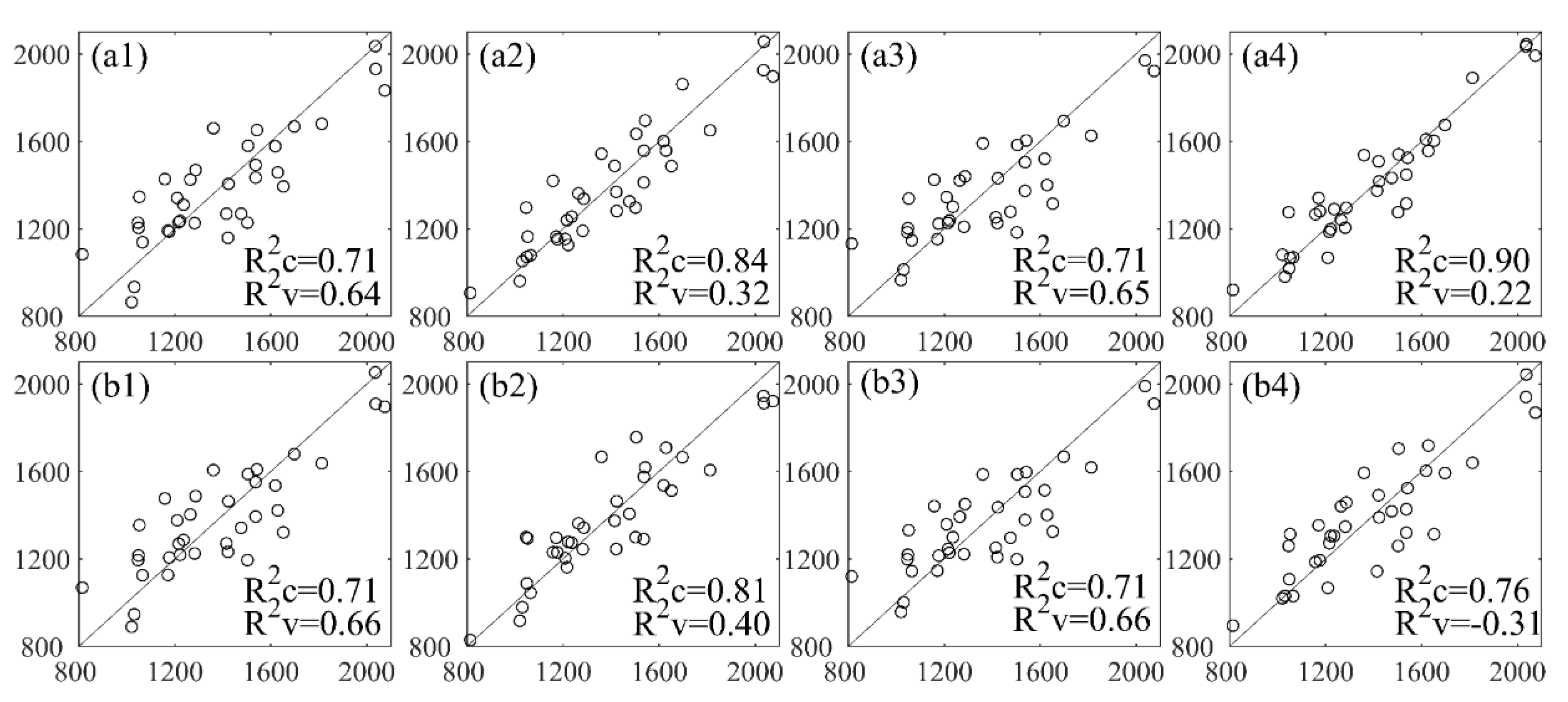
Table 2. The estimation accuracy of PLS models.
Spectral FormLVsSpectral RegionR2cR2vRMSEcRMSEv
R2Full wavelength0.71120.6402162.7501181.6767
R2Sensitive bands0.70810.6633163.6195175.7395
R’5Full wavelength0.84270.316120.1107250.4794
R’5Sensitive bands0.80910.3997132.3331234.6535
ln(1/R)2Full wavelength0.71090.6561162.8487177.6151
ln(1/R)2Sensitive bands0.71270.6583162.3386177.0468
CR6full wavelength0.89810.221696.6815267.2057
CR6sensitive bands0.7600−0.3052148.3587346.0075
Publisher’s Note: MDPI stays neutral with regard to jurisdictional claims in published maps and institutional affiliations.

