Article

Quantitative Study of the Effect of Water Content on Soil Texture Parameters and Organic Matter Using Proximal Visible—Near Infrared Spectroscopy

1
Eau Terre Environnement, INRS, 490 rue de la Couronne, Quebec City, QC G1K 9A9, Canada
2
BioEngine Research Team on Green Process Engineering and Biorefineries, Chemical Engineering Department, Université Laval, Pavillon Adrien-Pouliot 1065, av. de la Médecine, Quebec City, QC G1V 0A6, Canada
3
Agriculture and Agri-Food Canada, Quebec Research and Development Centre, Quebec City, QC G1V 2J3, Canada
*
Author to whom correspondence should be addressed.
Remote Sens. 2022, 14(15), 3510; https://doi.org/10.3390/rs14153510
Submission received: 16 May 2022 / Revised: 7 July 2022 / Accepted: 12 July 2022 / Published: 22 July 2022
(This article belongs to the Special Issue Application of Hyperspectral Data in Ecological Environment)

Abstract

:
Continuous monitoring of soil quality is a challenging task in agricultural activity. To meet this need, scientists have succeeded in developing a quick and inexpensive method to characterize soil properties. Thus, spectroscopy has become a promising method for quantifying soil parameters. However, this method remains sensitive to several factors such as water content (WC). The present study aims to quantify the effect of WC on the estimation of soil texture parameters (sand, silt, and clay) and organic matter (OM) using spectroscopy. Reflectance measurements in the laboratory on 68 soil samples were performed by varying the WC in each sample. The analysis revealed a significant influence of WC on spectra acquired from visible to near infrared (V/NIR) spectroscopy data and that spectra can be divided into two classes. To quantify the effect of WC, calibration/validation steps were performed on soil texture parameters and OM with and without taking WC into account. Calibration was performed using the partial least square regression algorithm, and the validation was assessed using four statistical evaluation indices (R2, Nash criterion (Nash), root-mean-square error (RMSE), and BIAS). Results showed a systematic increase in the accuracy of all studied soil particles when the WC is considered. Clay and OM were less influenced, while silt and sand were much more influenced by the WC. The study also highlighted that estimates of soil texture parameters using V/NIR data achieved relatively higher levels of accuracy (R2 > 0.80 and Nash > 0.80) than OM estimation (R2 = 0.83 and Nash = 0.78).

Graphical Abstract

1. Introduction

Soil areas are increasingly shrinking worldwide. Brabant [1] stated that there will be only 0.20 hectares per capita left in the world by the year 2100 if population growth and soil degradation continue at the current rate. Soil is one of the most important resources for the development of agriculture and the preservation of the environment because it plays an important role in water and carbon storage as well as temperature regulation. In addition, it is the source of nutrients for plants and is the habitat of micro-organisms responsible for the decomposition of organic matter [1]. Therefore, it is important to preserve this resource through continuous monitoring of its quality. Soil properties such as structure, aggregation, water retention, infiltration capacity, nutrient sorption, resistance to root penetration, microbial activity, soil carbon turnover, susceptibility to erosion and compaction, and ultimately the suitability of the soil for agricultural and forestry production are all closely related to soil texture and organic matter (OM). Therefore, they are considered the most important components used to determine soil quality, as it determines the physical, chemical, and biological properties of the soil quality [2].
Standard soil texture parameters and OM monitoring programs currently in use rely on in situ sampling techniques that are laborious, expensive, and limited in time and space; analysis involves sieving and sedimentation of suspended soil in solution. As an alternative, the visible and/or near infrared (V/NIR) spectroscopy data has been tested and used to this purpose [3]. The advantages of V/NIR data over standard monitoring programs are numerous (inexpensive, simple to implement, and non-polluting). In fact, V/NIR spectroscopy measures the interaction of radiation with matters (e.g., soil texture and OM) by absorption, emission, or reflection along the electromagnetic spectrum [4]. These characteristics allow it to record the spectral variations of optically active elements along the V/NIR spectrum and to identify chemical substances or functional groups in solid, liquid, or gaseous form. Therefore, spectroscopy spectra can be used to detect differences among soil particles.
In fact, the potential of the spectroscopic method to model the physical [5], chemical [6], and biological [7] properties of soil is well established. Many researchers have attempted and succeeded in modeling soil quality parameters, including soil textures and OM using V/NIR [8,9,10]. However, differences in the accuracy have been found between estimates resulting from field and laboratory acquisition of spectra. This is probably due to the sensitivity of the spectroscopy to environmental factors such as water content (WC) in soil. Indeed, water causes a general decrease in reflectance and an increase in an absorption peak located in the 1400 and 1900 nm region of the electromagnetic spectrum [11]. The refractive index of wet soil is lower than that of dry soil [12]. This decrease in the refractive index at the soil-water-air contact points causes consequently a decrease in the scattering of incident light compared to dry soil. In addition, the layer of water surrounding the soil particles produces additional reflection of the energy scattered in the water–air interface, producing more energy that propagates deeper into the soil [13].
In the context of soil modeling using spectroscopy-based data, in most cases, soil samples undergo a drying process to reach a dry state before their spectra are acquired and analyzed. The accuracy of the estimates is therefore high for dry soils but tends to be less accurate for different levels of soil WC. As explained in the section above, soil WC plays an important role on the intensity of the V/NIR spectral response. Consequently, it influences soil physicochemical parameters estimation. Therefore, some authors have separated the analyses according to groups of moisture content levels [12], removed the effect of water from the estimation of soil parameters [14] or quantified the effect of WC on the spectra recorded in the field as well as those recorded in the laboratory to estimate OM [15]. Despite the prominent role of WC on soil parameter modeling, its effect on soil texture parameters and OM modeling is yet very scarce.
This work attempts to quantitatively investigate the effect of soil WC on the accuracy of modeling soil texture parameters (sand, silt, and clay) and OM using the V/NIR spectroscopy data. The calibration step was performed using the partial least square regression algorithm. The generated models were evaluated using the bootstrap k-fold cross-validation technique. Accuracy was assessed using four statistical evaluation indices (R2, Nash criterion (Nash), root-mean-squares error (RMSE), and BIAS).

2. Materials and Methods
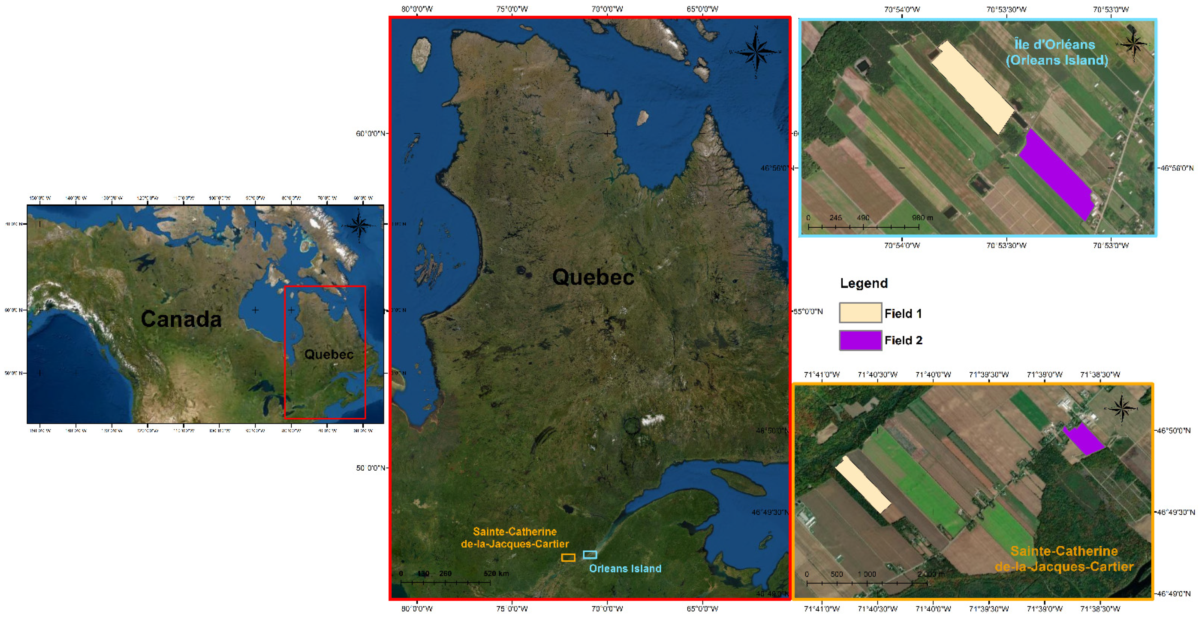
2.1. Study Area

Soil samples were collected by an Agriculture and Agri-Food Canada team from four fields: two located in Sainte-Catherine-de-la-Jacques-Cartier and two in L’Ile d’Orléans (Orleans Island; Figure 1). According to the Canadian classification, these samples were categorized into four soil series (Pont-Rouge, Morin, Orléans, and St-Nicolas) belonging to two broad classes (Orthic Humo-Ferric Podzol and Eluviated Dystric Brunisol). Orthic Humo-Ferric Podzolic soils have a brownish Podzolic B horizon with low OM content. They are common on less moist sites in the Podzolic soil region as well as on moist sites. They are generally found under coniferous, mixed, or deciduous forests, but may also be found under grass and shrub vegetation. Eluviated Dystric Brunisols generally have organic surface horizons and brownish acidic B horizons overlying acidic C horizons with an eluvial horizon at least 2 cm thick. These are acidic Brunisols that do not have a well-developed mineral-organic surface horizon. They are widespread, generally, on parent materials of low basal status and typically under forest vegetation.
A narrow range of soil parameters and texture types from the four fields (detailed in Table 1) are collected in this study. Soil texture ranged from loamy coarse sand (Sainte-Catherine-de-la-Jacques-Cartier fields) to coarse sandy loam (Orleans Island fields). These two classes are characterized by more than 25% of coarse and very coarse sand and less than 50% of any other sand grade. In other words, the proportion of sand in the collected samples, from all fields, is overrepresented compared to silt and clay.

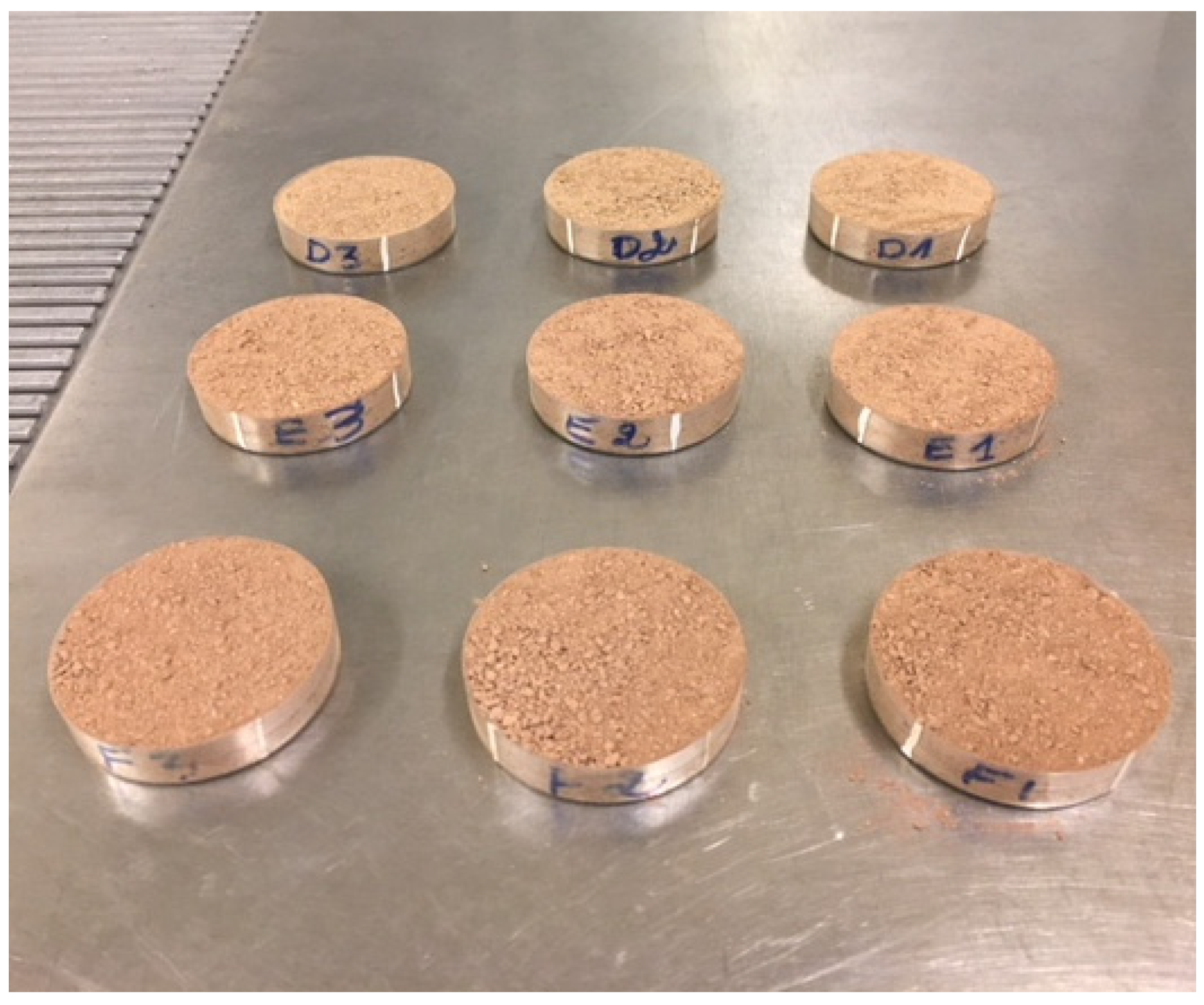
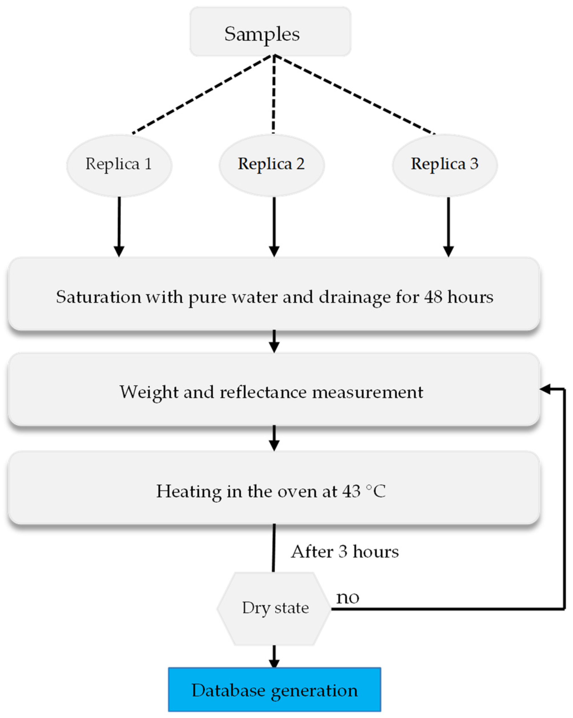
2.1.1. Soil Sample Preparation

Sixty-eight samples were collected for this study. Soil texture determination of these samples was then performed by an analytical team from Agriculture and Agri-Food Canada following a well-known procedure published by Kroetsch and Wang [17]. Each sample was after that divided into three plastic Petri dishes (PPD) of size 60 × 60 × 15 mm; the weights of the PPD were measured in advance (Figure 2). This step serves to account for the operator error while varying the WC of samples. The surface of samples was flattened with a metal spatula while avoiding squeezing the soil particles. This step reduces the multiplicative and additive effects associated with the roughness of the contact surface between the sample and reflectance probe. The PPD were then covered by a geotextile, which is a relatively thin membrane allowing the retention of all soil particles and allowing only water penetration. The covered PPD were afterwards placed upside down in a tray filled with pure water and were kept in this position for one hour. This operation allowed the saturation of the soil by capillarity phenomena without touching the surfaces of the PPD (where the reflectance measurements will be made). The samples were thereafter placed on a metal grid for 48 h to allow the water to drain and the soil to reach the WC at field capacity. Gravity water drainage time is between 24 and 48 h [18], and the choice of 48 h was made after several tests following the steps pre-described above.

2.1.2. Water Content Measurement

As the objective is to acquire soil spectra at varying WC levels, the samples were heated in the oven at 43 °C to keep the WC of all the soil particles approximately homogeneous and went through the same weight and reflectance measurement processes every 3 h for 24 h. This was performed to bring the soil samples to a dry state. Although Lekshmi [18] suggested that the dry state is reached for soil heated to 105 °C for 24 h, tests on our samples showed that there is no significant variation after 24 h of heat at 43 °C, and therefore, no variation in soil weight was observed after 24 h. The WC computation for each weight measurement, for each replica, was performed using Equation (1). Figure 3 summarizes all steps undergone for generating the database. It is important to mention that before starting the above process, the weight of each replica was measured by an electronic balance.
θ = w e t   w e i g h t i d r y   w e i g h t d r y   w e i g h t × 100
where θ is volumetric water content (WC) in percent, w e t   w e i g h t i (gram) are weights of samples in all WC levels other than dry measured (i: 3 h:24 h), and d r y   w e i g h t (gram) is the weight of the samples after 24 h of heating in the oven at 43 °C.

2.1.3. Reflectance Measurement

The reflectance of the soil samples was measured by the Ocean Optics system. This system is composed of six main parts: (1) a dark support in contact with the surface of the soil sample and on which the probe has been fixed to prevent stray light from reaching it. This support is also used to keep a constant distance (1.7 cm) between the probe and the soil surface during the acquisition of the spectral signature; (2) an HL-2000 halogen lamp which represents the light source; (3) two spectrometers allowing the measurement of the reflectance on two different spectral ranges. One spectrometer operates in the visible range and part of the NIR (340–1038 nm) with a spectral resolution of 0.4 nm. The other operates in the NIR (900–1700 nm) with a spectral resolution of 3 nm; (4) a premium reflection probe connected at one end to eight optical fibers that carry light photons from the halogen lamp to it, and at the other end it is connected to a single optical fiber whose role is to transfer the amount of energy reflected from the soil sample (captured by the probe) to the spectrometer; (5) a reference characterized by a total reflectance (reflectance equal to 100%) for the calibration of the spectrometers; and (6) the OceanView software (Ocean Insight, Orlando, FL, USA) for acquisition, reading, and storage of spectra (Figure 4).
The acquisition parameters were set so that the software would average two internal acquisitions to reduce the signal-to-noise ratio. For each replica, four measurements, in four different points (approximately one point every 45° of the ground surface circle), were acquired. After 20 reflectance measurements, the software was recalibrated again to remove the material derivative.

2.2. Statistical Methods and Evaluation Indices

2.2.1. K-Means Unsupervised Classification

The K-means is a non-hierarchical data partitioning algorithm based on moving centers. The computational principles of this algorithm can be summarized in four basic steps: (1) choose arbitrarily “n” individuals who will be the centers (or kernels) of the classes; (2) assign each observation in the database to one of the “n” classes whose kernel is the closest; (3) recompute the new centers of gravity for each class; (4) check if the centers and classes change or the maximum number of iterations is reached. If these two conditions are not verified, the computation continues starting from step #2 [19].

2.2.2. Correlogram

In data analysis, a correlogram is a graphical representation highlighting one or more correlations between the data sets. A correlogram can be used to visualize data in different forms. The forms often used in graphical representation are plots (2-dimensional (D) or 3-D graphs) or 2-D matrices. The goal, however, is to facilitate decision making in the modeling process.

2.2.3. Principal Component Analysis (PCA)

The basic idea of PCA is the dimensionality reduction in data in which there are many interrelated variables while keeping the maximum variance in the new variables (principal components). This reduction is achieved by projecting the variables onto a new space so that the latter are uncorrelated, and the former retain the maximum amount of information present in the original variables [20]. Therefore, this method serves to concentrate the information stored in large databases by representing it in a reduced space (2- or 3-D space). This also allows the identification of similarities between samples and thus facilitates identifying the groups of individuals as well as the determination of links between variables.

2.2.4. Classification and Regression Tree (CART)

Developed by Breiman et al. [21] in the 1980s, the CART method is widely used for classification and regression purposes. To build decision trees, the CART uses a learning sample, composed of a set of historical data with pre-assigned classes for all observations and a set of splitting variables. These decision trees are used afterwards to classify new data. Classification trees are built in accordance with a splitting rule, which splits learning samples into smaller groups of maximum homogeneity. The maximum homogeneity of child nodes is determined by the impurity function, which can be calculated by either the Gini or the Towing splitting rule.

2.2.5. Partial Least Squares Regression (PLSR)

The PLSR is a method for constructing predictive models when the factors are highly collinear [22], such as the case of spectroscopy data. It is an iterative statistical technique developed by Wold [23]. Similarly to PCA, the PLSR acts to relate data matrices using a linear multivariate model and subsequently reduce collinearity and noise within a data set [24]. This two-step technique moderates the predictors of a data set to a smaller set of uncorrelated components and performs least squares regression on these components rather than on the original data.

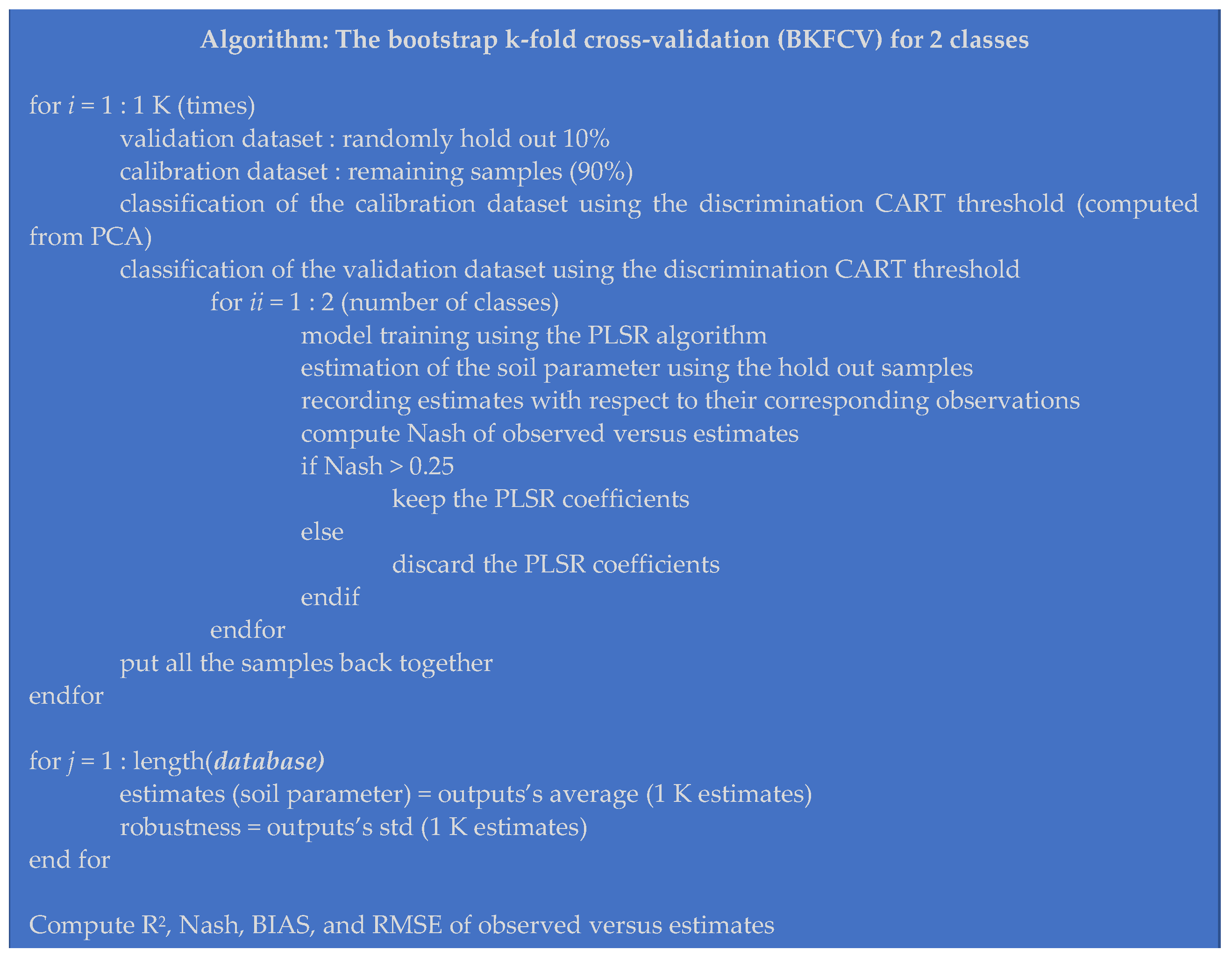
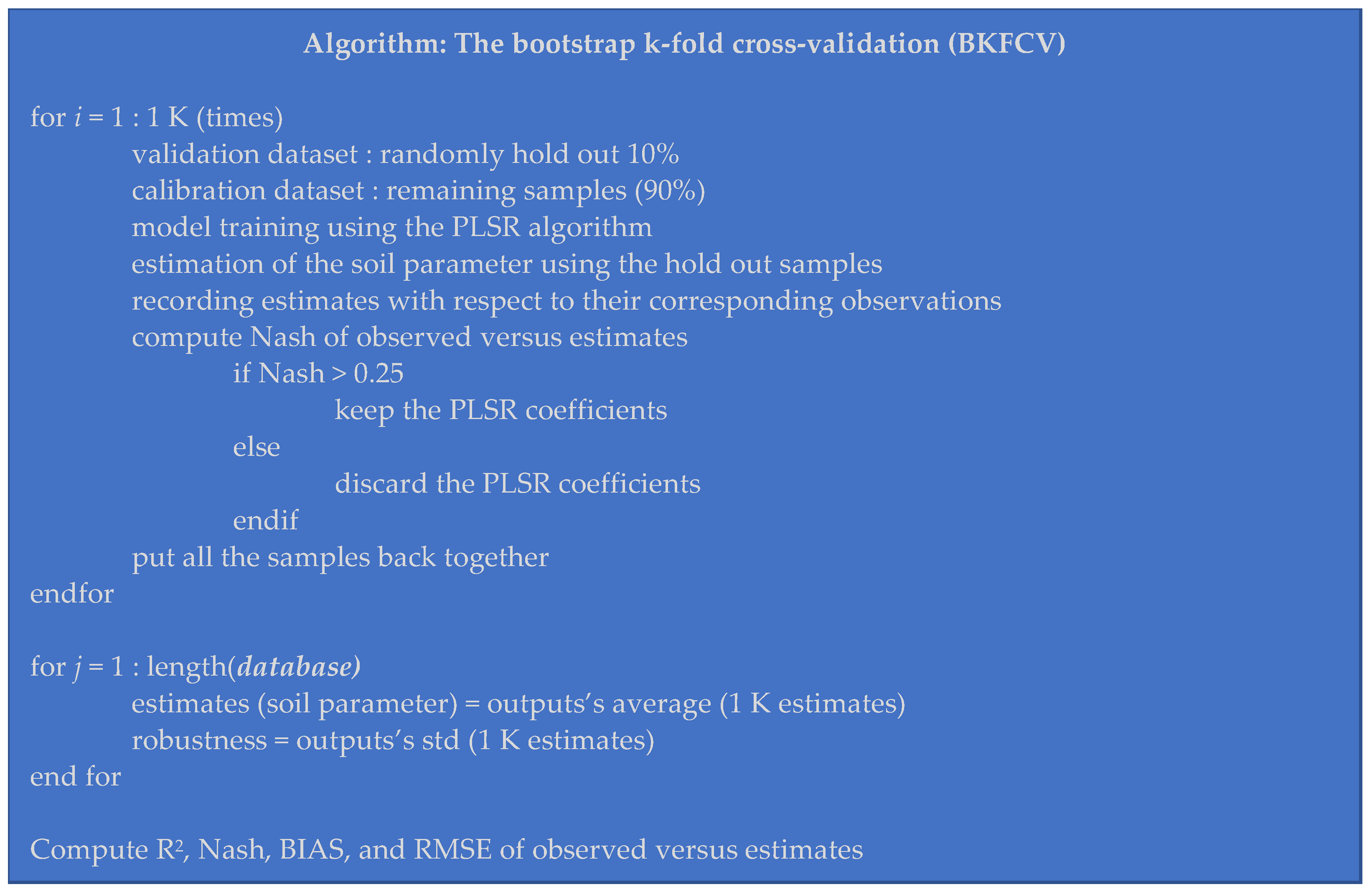
2.2.6. Bootstrap k-Fold Cross-Validation (BKFCV)

In statistics, bootstrap techniques are statistical inference methods based on multiple replication of data from the dataset under study, using resampling techniques [25]. The cross-validation is a resampling procedure used to evaluate machine learning models on a limited data sample. The procedure has a single parameter called “k” that refers to the number of groups into which a given data sample should be divided. As such, the procedure is often referred to as k-fold cross-validation [26]. This technique is mainly used in applied machine learning to estimate the accuracy of a machine learning model on unseen data. The general procedure is as follows: (1) randomly shuffle the database and divide it into k groups; (2) hold out the observations of group-1 as the test data set and use the observations of the remaining groups as the training data set; (3) fit a model with the training dataset (k-group-1) and evaluate it with the observations of the hold-out group (group-1) by the fitted model function; (4) save the estimates of group-1 and discard the fitted model; (5) put group-1 back into the database and hold-out group-2; (6) repeat steps (2) to (5) until group-k is reached [26]. It is important to note that each observation in the sample data is assigned to an individual group and remains in that group for the duration of the procedure. This means that each sample is used one time in the holding set and used to train the model k-1 times (Figure 5).
The BKFCV is a combination of these two methods developed specifically to this study. It is a resampling (bootstrap) technique and a k-fold cross-validation (or split technique) that uses a group of the database as the training data set and the remaining observations as group of the test data set. However, unlike k-fold cross-validation, once the model is fitted with the training dataset (size of the database-group-x (k-fold)) and evaluated with the samples from the hold-out group-x (step 3 of k-fold cross-validation), the samples of the group-x are put back into the training dataset and another test dataset (group-y) is randomly held out and the remaining samples (size of the database-group-y (k-fold)) are used as the training dataset, and so on until the number of the bootstrap iterations is reached (set to 1 K in this study). The advantage of this technique is that the estimations (the outputs of the different trained models) are evaluated several times by their corresponding observations. It allows us also to quantify the robustness of the modeling process. Indeed, the use of this technique allows us to calculate the variance of the estimates at each observation; the lower the variance is, the more robust the estimates are.

2.2.7. Statistical Evaluation Indices

Four statistical evaluation indices (coefficient of determination (R2), Nash criterion (Nash), root-mean-square error (RMSE), and BIAS) were used (Equations (2)–(5)). The Nash criterion evaluates the performance of the models by comparing the estimated values with the average of the measured ones. For a negative Nash, it would be better to use the average of the measured values than those estimated by the model, which is very poorly performing. The model starts to be satisfactory at Nash ≥ 0.60. A Nash ≥ 0.80 in the modeling is considered good. The model is perfect for Nash = 1 [27].
R 2 = [ i = 1 n ( M i M ¯ ) ( Es Es ¯ ) i = 1 n ( M i M ¯ ) 2 i = 1 n ( Es i Es ¯ ) 2 ] 2
BIAS = 1 n i = 1 n ( Es i M i )
RMSE = 1 n i = 1 n ( Es i M i ) 2
NASH = 1 i = 1 n ( M i Es i ) 2 i = 1 n ( M i M ¯ ) 2
where n is the sample size, M and Es are the measured and estimated values, and M ¯ and Es ¯ are the averages of the measured and estimated values.

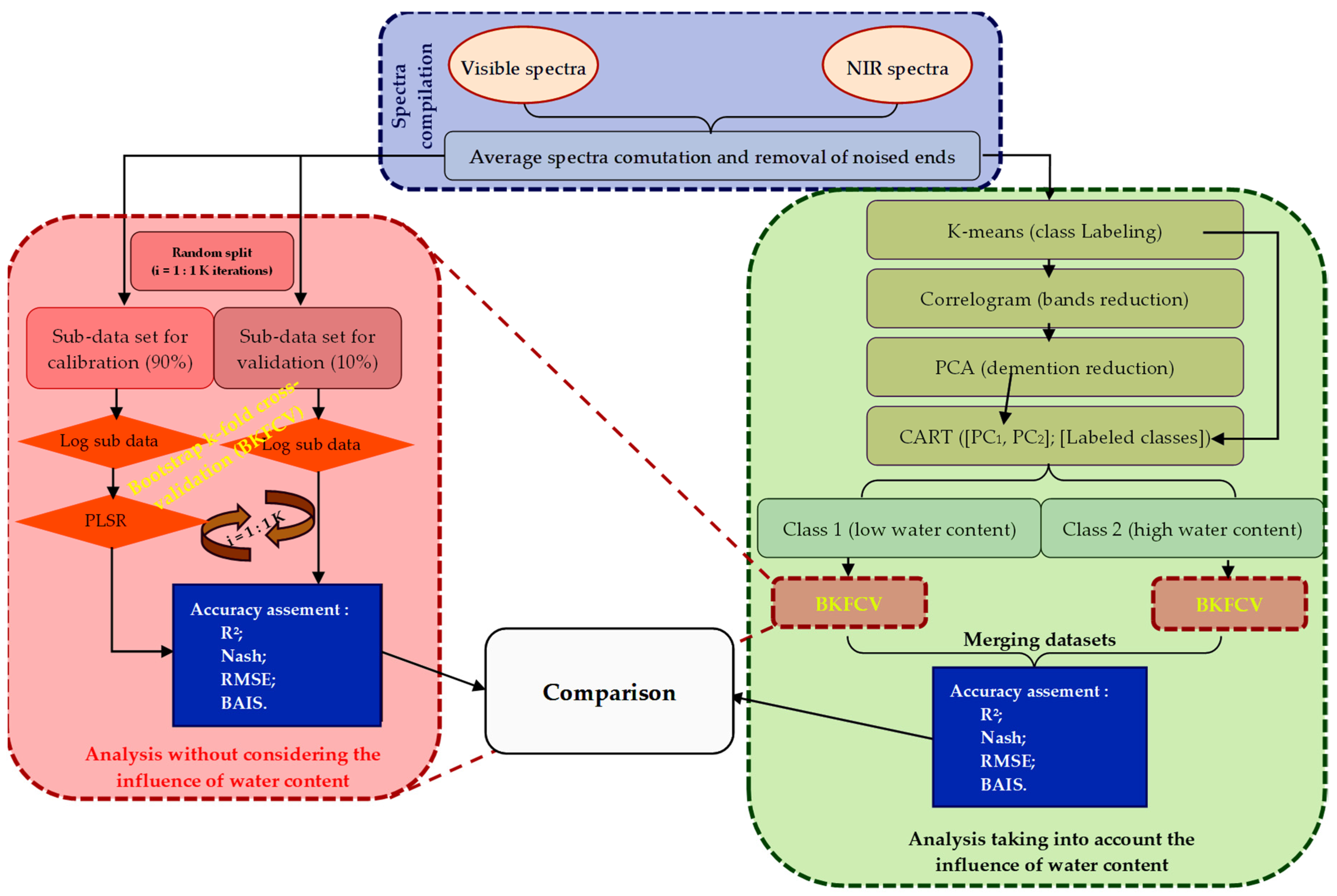
2.3. Methodological Approach

Since the V/NIR spectra were acquired separately, observations with missing visible or NIR spectra were removed from the database, leaving a total number of 1025 observations. Then, samples with fewer than 3 replicates were removed in the averaging step of their spectra. In addition, the number of wavelengths was reduced via a moving average of one quarter, one sixth, one eighth, and one tenth for each domain (visible and NIR) to reduce the roughness of the raw signal. Assuming the reduction factor is f, this operation consists of assigning the average of the reflectance j to j + (f − 1) at wavelength j. The choice of the reduction factor applied to the visible and NIR wavelengths was based on the appearance of the spectra (smooth signature) provided. At the end of these compilation processes, the final database size was 288 observations.
Once the database compiled, two analyses were conducted. The first was to evaluate the accuracy of modeling soil texture parameters and OM taking into account the influence of WC. To do so, it was necessary to develop a classifier allowing us to discriminate between samples with a high and low WC. An unsupervised k-means classification was applied. The number of individuals was set to 2; the choice of using two classes in explained in Section 3.2.1 (“K-means Unsupervised Classification”). This step allowed us to label two classes of spectroscopy data with respect to WC. Next, a correlogram was computed. The correlogram was used to quantify the correlation between the V/NIR spectroscopy data and WC. The highly correlated bands (R2 > 0.85) were retained, and the others were discarded. Once the bands were selected, a PCA was applied on these bands for dimensionality reduction. The first two principal components were then used in a CART algorithm with the pre-labeled classes obtained from the k-means classification. Once the classifier was developed, it was possible to spectrally divide the database into two classes (high and low WC). For the BKFCV purpose, the following steps were performed:
1.
Hold out 10% of the database for validation.
2.
Classification of the 90% into two classes using the discrimination threshold.
3.
For each class, the following steps were applied:
  • Training using the PLSR algorithm.
  • Classification of the validation data set (10%) using the discrimination threshold.
  • Estimation of the corresponding soil parameters using the calculated PLSR parameters (coefficients and intercept) corresponding to each class.
  • Recording of the estimates with respect to their corresponding observations.
4.
Record the calculated PLSR parameters if the Nash is higher than 0.25 and put all observations back together.
5.
Repeat steps 1:4 1 K times.
At the end of the iterations, each observed value had a set of corresponding estimates. These underwent the following calculations for each class separately and by combining the two classes:
  • Compute the averages of estimates that were challenged with their corresponding observations to evaluate the modeling process using statistical evaluation indices (R2, Nash, RMSE, and BIAS).
  • Compute the variances of estimates to assess the robustness of the modeling for each observation (Figure 6).
The second was to evaluate the accuracy of modeling soil texture parameters (sand, silt, and clay) and OM using hyperspectral data without considering the influence of WC. To do so, the BKFCV algorithm was used by the following steps:
  • Hold out 10% of the database for validation purposes.
  • Train the remaining 90% using the PLSR algorithm.
  • Estimate the corresponding soil parameters using the calculated PLSR parameters (coefficients and intercept).
  • Record the estimates with respect to their corresponding observations.
  • Record the calculated PLSR parameters if the Nash is higher than 0.25 and put all observations back together.
  • Repeat steps 1:5 for 1 K times.
For the modeling evaluation, averages and variances were calculated as described previously (Figure 7).
Finally, for the comparative analysis, the means and variances calculated in this step (as in the case where the effect of WC is not taken into account) were compared to the results of the two classes studied previously (as in the case where the effect of WC is taken into account). To ensure consistency in the comparison analysis, the results of the two classes were combined, and the four evaluation indices were recalculated. The flow chart in Figure 5 summarizes the steps of the methodological approach (Figure 8).

3. Results and Discussions

3.1. Database Compilation and Description

3.1.1. Soil Properties
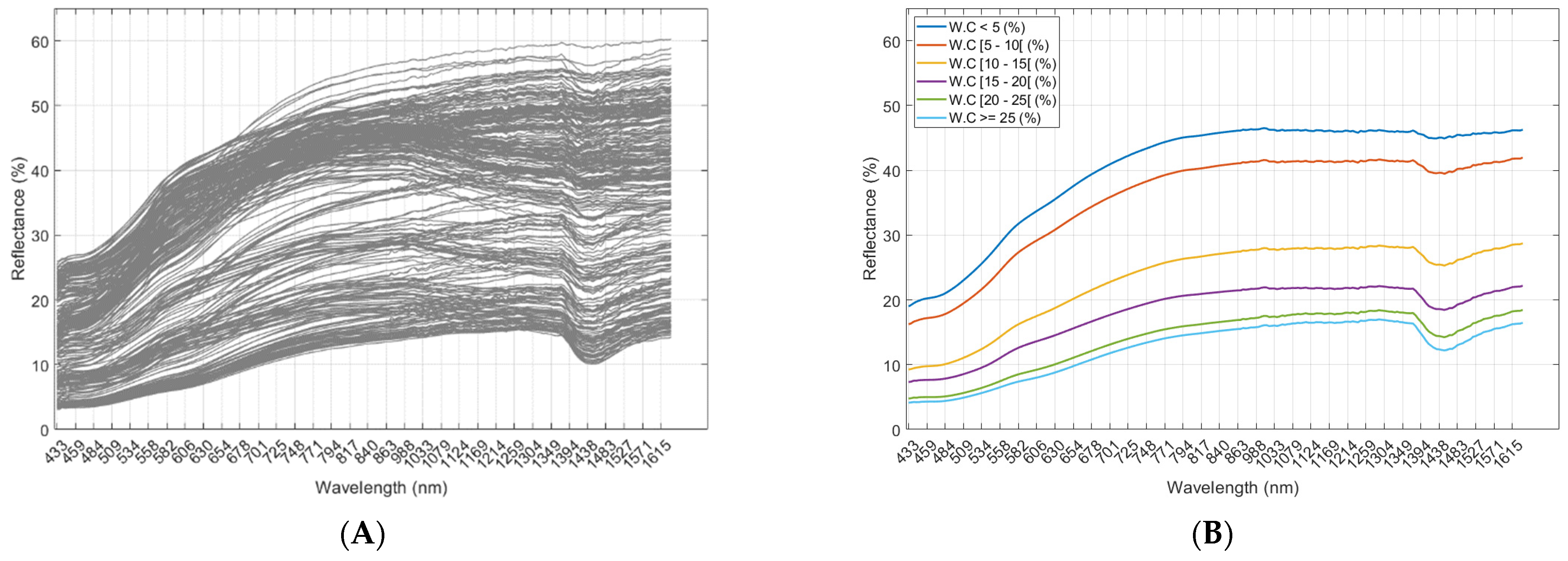
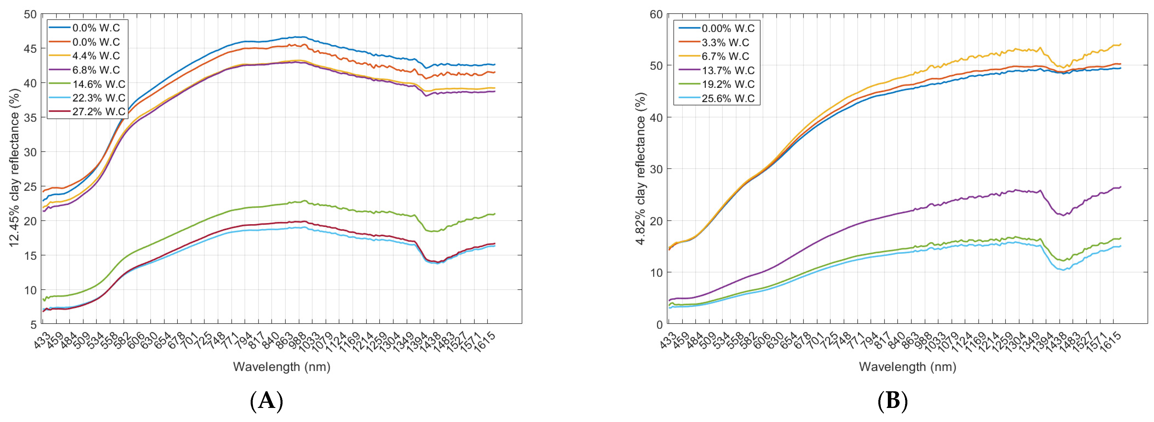
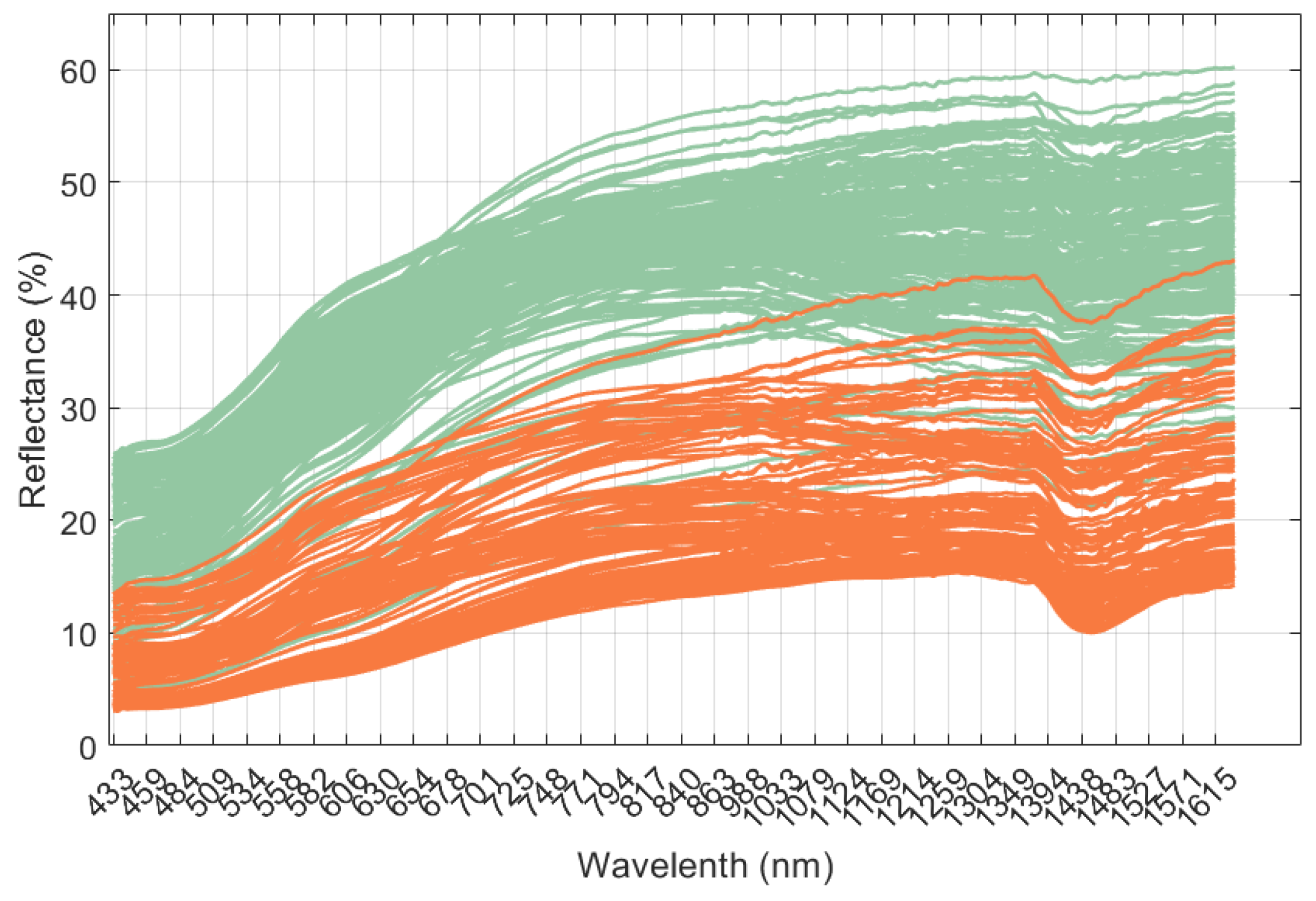
The size of the soil parameters database was 288 observations (Table 2). A wide range of WC was covered in this study. The standard deviation for clay and OM is narrow, while it is wide for sand and silt. From a modeling point of view, this narrowness could be a limiting factor to achieving good performance since the modeling process is data-oriented.

3.1.2. Soil Spectra

The spectral behavior along the spectrum is typical of soil, characterized by a continuous increase in the reflectance magnitude from blue to NIR with an absorption dip around 1400 nm (Figure 9A). Hunt [28] has also highlighted this absorption of light energy around 1454 nm, among others, and related it to the overtones of the O-H molecules of water and the combinations of vibrational modes of liquefied water when excited by radiation frequencies in these NIR ranges. To verify this finding, the database was subdivided into 6 (<5%, [5–10%[, [10–15%[, [15–20%[, [20–25%[, ≥25%) WC intervals. Our results (Figure 9B) also show that there is a clear dependence relationship between the soil WC and the absorption dip around 1400 nm, as suggested in the literature.

3.2. Modeling Soil Texture Parameters Taking into Acount the Influence of Water Content

3.2.1. K-Means Unsupervised Classification

Since k-means is a non-hierarchical data partitioning algorithm, and the number of classes must be defined. However, the number of classes was not known beforehand. A spectral analysis had to be performed for this purpose. Therefore, to analyze the effect of WC on spectra, each percentage of soil sample textures was plotted. Figure 10 shows two examples of these plots. In Figure 10A, the spectrum of 12.45% clay (equivalent to 32.99% silt, 54.55% sand, and 4.09% OM) depending on the variation in WC after 3 h heating for 24 h is shown as an example of high clay content. In Figure 10B, the spectrum of 4.82% clay (equivalent to 14.22% silt, 80.97% sand, and 4.15% OM) depending on the variation in WC after 3 h heating for 24 h is presented as an example of low clay content. In both examples, two batches of spectra are well distinguished. A batch of dry soils, characterized by the absence of the absorption dip around 1400 nm and a higher reflectance along the spectrum, and a batch of wet soils, characterized by the absorption dip around 1400 nm and a lower reflectance along the spectrum. Based on this analysis, it was hence decided to set the number of classes to two when using the k-means classification.
Two classes of spectra are well distinguished. The green likely related to samples with low WC (dry soils) and the orange likely related to samples with high WC (wet soils). However, there exists an area of confusion between the two classes (Figure 11). It is important to keep in mind that the portions of the soil texture in each sample are different. The soil spectra may react differently, in some cases, depending on the rate of each element in the soil sample being scanned. The example in Figure 10B is perhaps the most appropriate for further explanation. The sample at 6.66% WC is in the dry soil batch, while its spectrum shows a clear dip around 1400 nm, specific to wet soils. This is likely related to the amount of sand (≈80%) in this sample. Sand is highly reflective compared to silt and clay. Thus, the amplitude of the reflectance is higher. On the other hand, this sample still has about 20% silt and clay. These elements are known to be very water retentive. Therefore, the presence of the dip around 1400 nm.

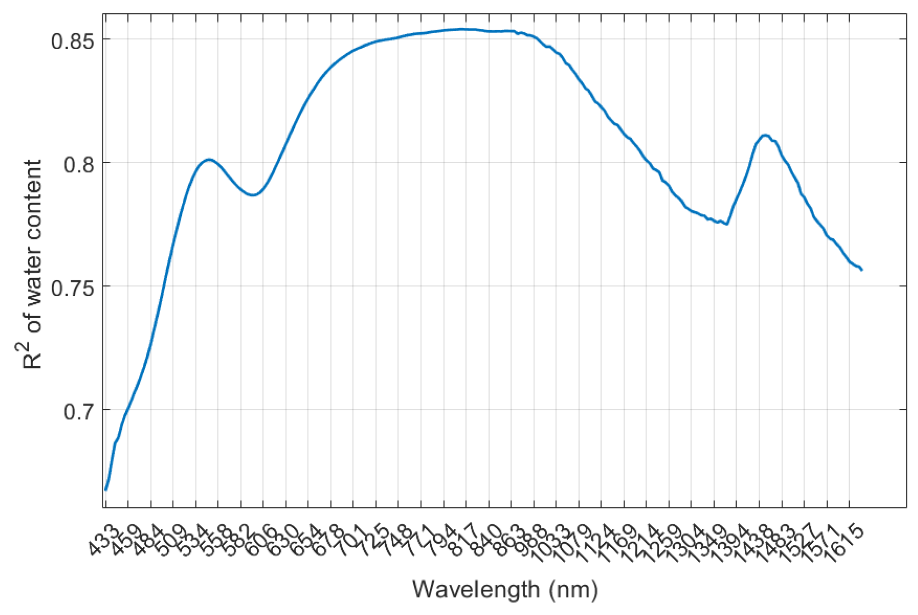
3.2.2. Water Content and Spectroscopy Data Correlogram

As mentioned earlier, correlograms are the best way to present data for analysis and to highlight one or more relationships between a data set. The purpose of this step was to identify the most sensitive (highly correlated) spectral regions to WC before applying the PCA algorithm. This will allow us to compute principal components that are uniquely sensitive to WC. It is very important to compute principal components that are as unaffected by noise from the other soil parameters (sand, silt, clay, etc.) as possible, as the first two will be used with the CART algorithm to develop our classifier. Contrary to expectations, the bands around 1400 nm were not the most correlated with the WC. The bands at the end of the visible range were the most correlated (Figure 12). This is most likely due to the high percentage of sand in the studied samples. The water retention capacity of sand is known to be low, and the dip around 1400 nm is very much related to the O-H molecules in water, which are generally more abundant in silt and clay. This may explain the relatively low correlation between WC and the wavelength around 1400 nm. Therefore, wavelengths with R2 > 0.85 were selected and used for the PCA calculation.

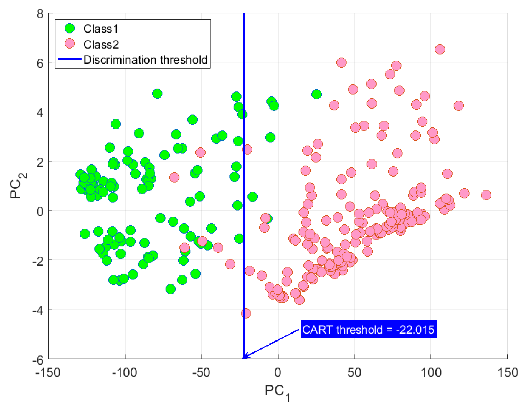
3.2.3. Classifier Parametrization

To develop the classifier that allows spectral discrimination between the two pre-identified classes, a PCA was first applied on the selected bands. The first principal component (PC1) explained 99.91% of the variance. For visualization purposes, the first two principal components (PC1 and PC2) are shown in Figure 13. A clear discrimination pattern is observed along the PC1. There is an area of confusion between the two classes, which is likely related to the spectra confusion discussed in the section above. PC1 and PC2 are orthogonal, which highlights the lack of dependence between the two variables (collinearity). In fact, efficiency of multivariable classification highly depends on correlation structure among predictive variables. When the covariates in the model are not independent one to another, collinearity problems arise, which leads to biased classification [29]. As mentioned earlier, the CART requires a set of partition variables, which are PC1 and PC2, in our case, and a training sample composed of a data set with pre-assigned classes for all observations. The unsupervised k-means classification result was used for this purpose. As expected, the CART algorithm utilized CP1 for discrimination of the two classes. The discrimination threshold is set to −22.015 (blue line in Figure 13).

3.2.4. Results of the Bootstrap k-Fold Cross-Validation (BKFCV)

Clay Percentage Estimates in Each Class

In both classes, for high (Figure 14A) and low (Figure 14B) WC, good accuracy is achieved. The R2 and Nash were greater than 0.80 and the RMSE was less than 1.07%. The high-WC observations achieved the best performance (R2 = Nash = 0.86; Figure 14B). The scatter points around the 1:1 line in both classes emphasize that the estimates tend to be slightly underestimated for high values percentage, particularly for low-WC (Figure 14B). The variance bars also tend to be wider with high percentages for both classes, reflecting the less robust modeling of these values compared to the low clay percentages.

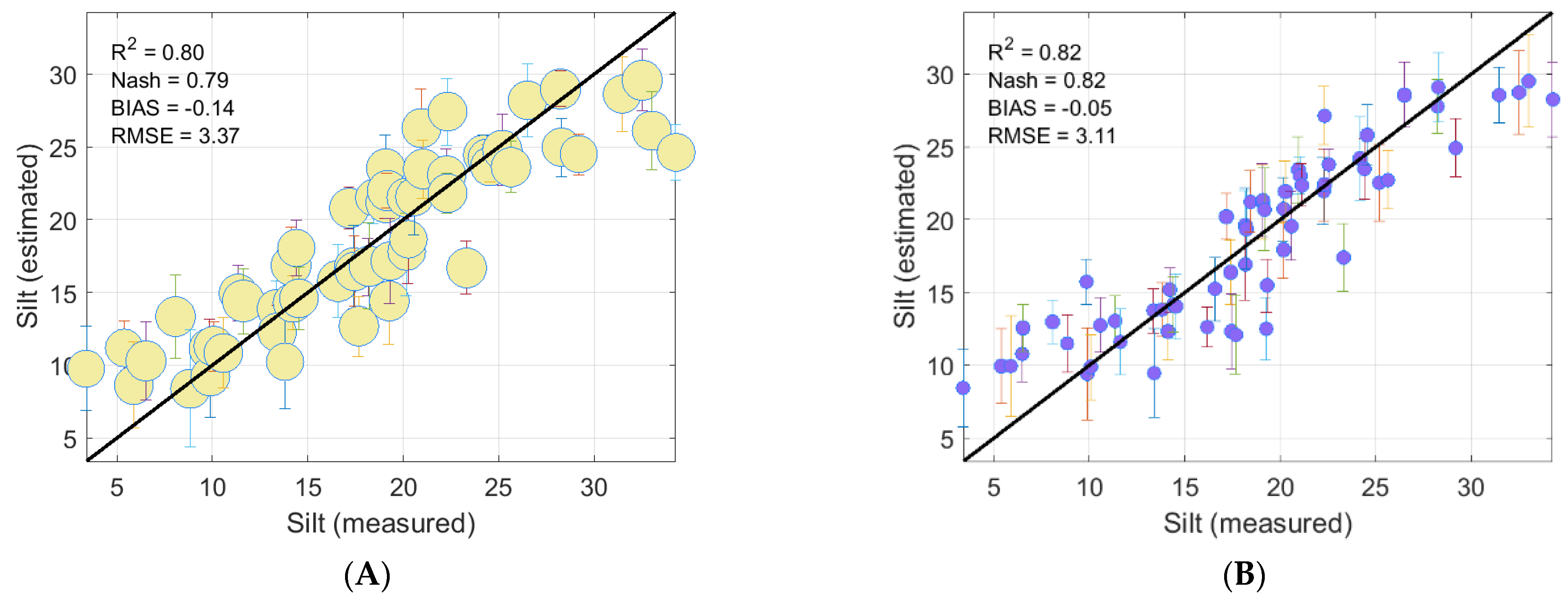
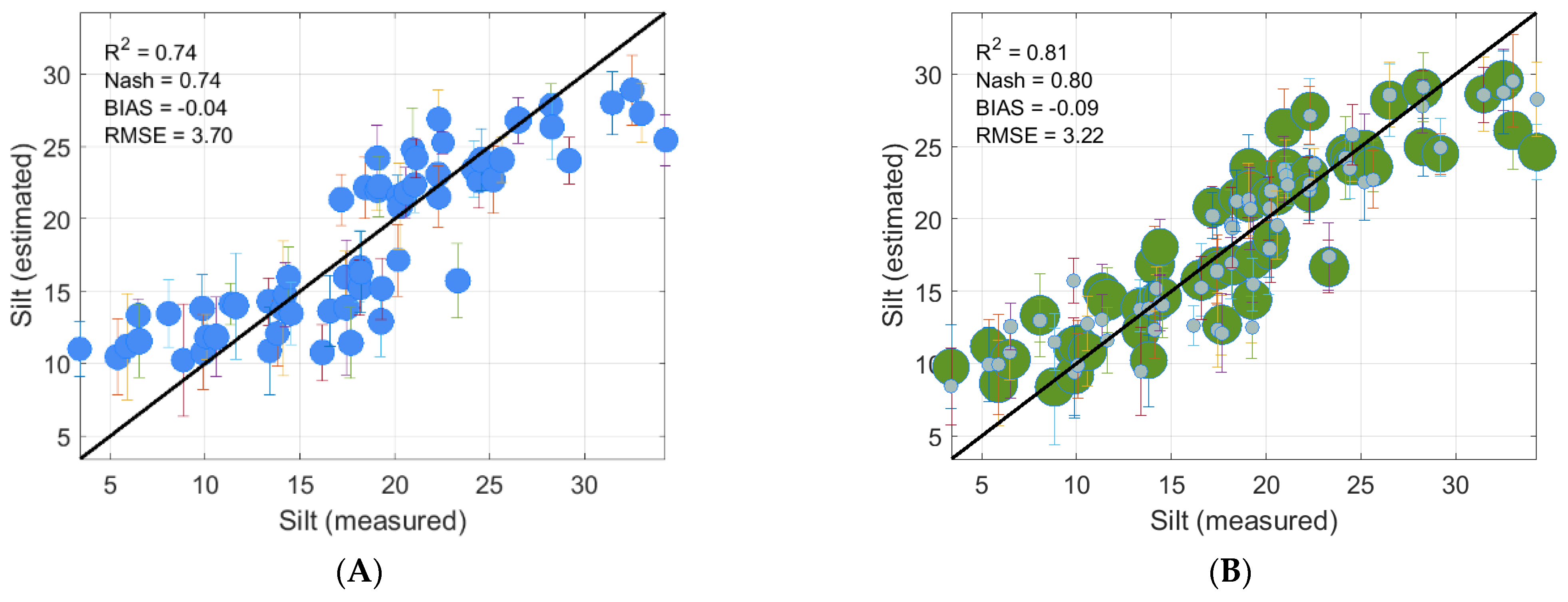
Silt Percentage Estimates in Each Class:

In both classes, for high (Figure 15A) and low (Figure 15B) WC, a relatively lower accuracy than the percentage estimate of clay is obtained, but it is still high. The R2 and Nash were greater than 0.79 and the RMSE was less than 3.37%. Unlike the clay percentage, the low-WC observations achieved the best performance (R2 = Nash = 0.82; Figure 15B). The scatter points around the 1:1 line in both classes emphasize that the silt tend to be slightly underestimated for high percentages and relatively overestimated for low percentages. The variance bars are narrower in the central modeling space (values between 15 to 25%) and wider at both extremities. This makes perfect sense, as the central values are well distributed around the 1:1 line (case of high modeling robustness), while the extreme values are located either above (case of overestimation) or below (case of underestimation) the 1:1 line, highlighting lower modeling robustness.

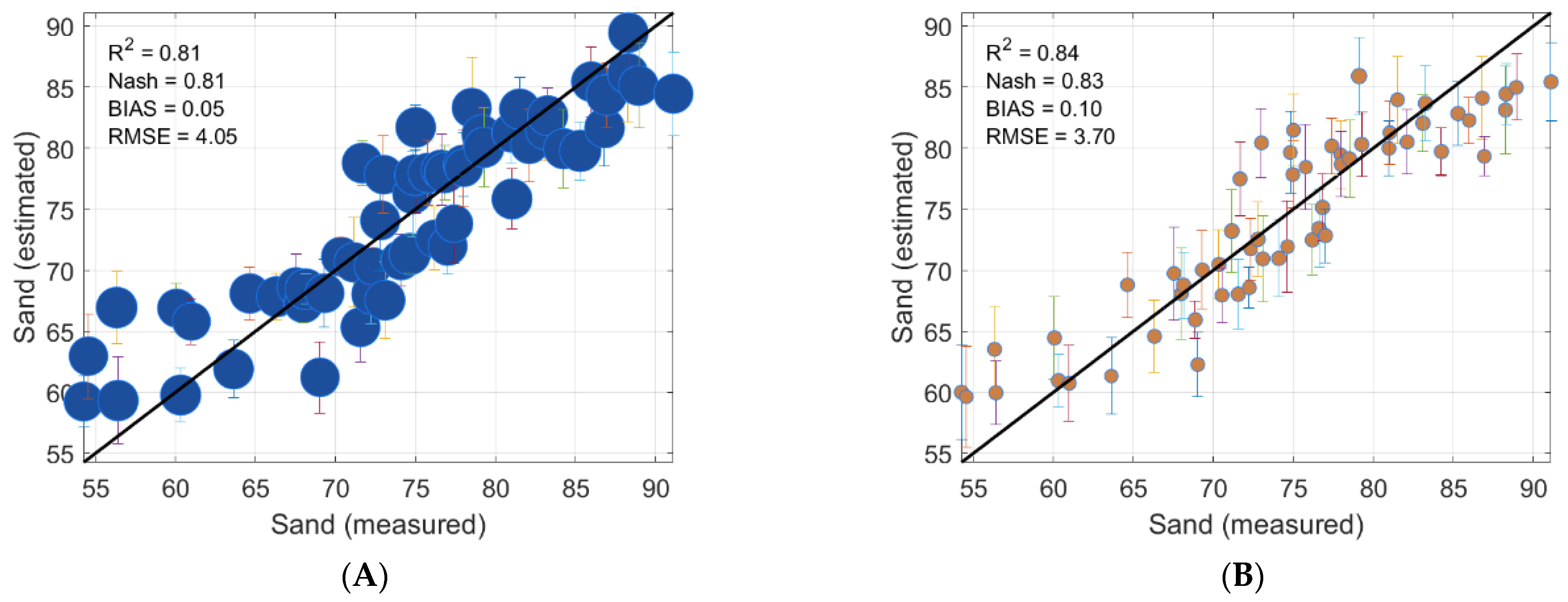
Sand Percentage Estimates in Each Class:

Accuracy performance of sand percentage estimate is quite equal to clay. The R2 and Nash were greater than 0.81, and the RMSE was less than 4.05%. Unlike the clay percentage, the low-WC observations achieved the best performance (R2 = 0.84 and Nash = 0.83; Figure 16B). However, a lack of quality estimates is apparent for low percentages (<70%), especially for observations with high WC (Figure 16A). This is likely because the range of sand percentages is higher than that of clay and silt (10%, 30%, and 37% for clay, silt, and sand, respectively). This could have created two different observation populations in the sand samples. Furthermore, the sum soil textures must be 100%, samples with less than 70% sand (where estimates are subject to error) must imperatively contain 30% to 50% clay and silt. Knowing that the physicochemical mechanisms and WC retention capacity of sand are not the same as those of clay and silt, this probably made the V/NIR spectra responses of the group of samples with 70% sand and above different from those with a lower fraction of sand (50% to 70%). The presence of large amounts of silt and clay must have interfered with the spectral signature and influenced the sensitive regions for sand detection. As for the two soil textures above, the error bars are larger at the extremities, especially for low percentages in both classes.

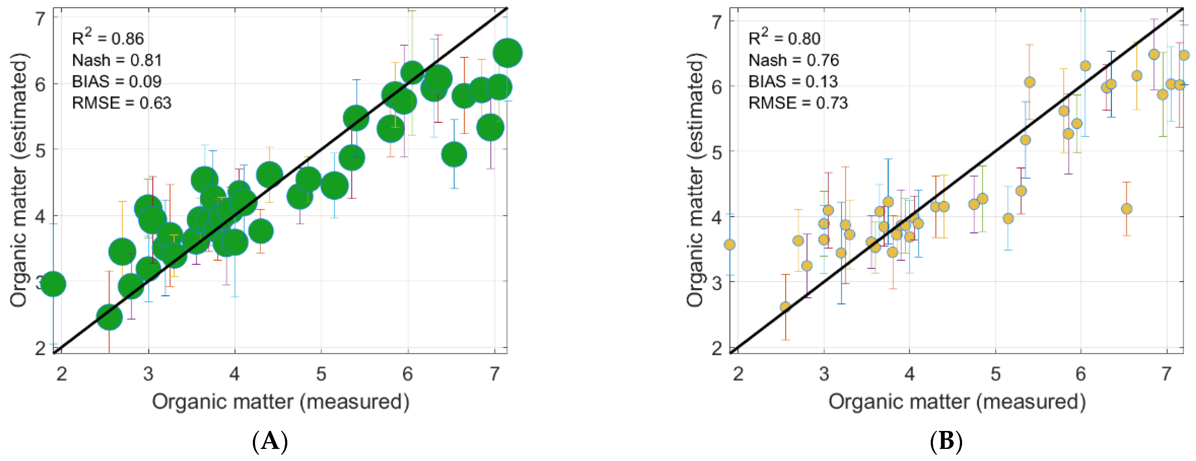
Organic Matter Percentage Estimates in Each Class:

Accuracy performance of OM percentage estimate is quite equal to the other soil textures in terms of R2 (>0.80). However, a clear decrease in Nash results, which is much more severe statistical evaluation index, is perceived (Figure 17B). The OM percentage with the high-WC observations achieved the best performance (R2 = 0.86 and Nash = 0.81; Figure 17A). In both classes, the scatter points around the 1:1 line are well distributed with a slight tendency of overestimation for low percentages and underestimation for high percentages. Nevertheless, one to two observations in each class are far from the 1:1 line, which explains the poor modeling performance assessed by Nash. Compared to the soil textures, error bars are in most cases wider, notably at the extremities.

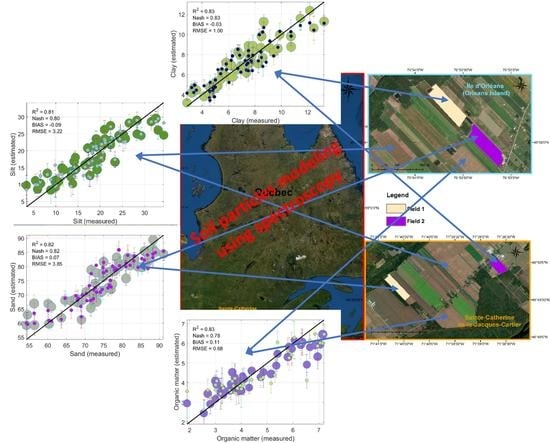
3.3. Modeling Soil Texture Parameters with and without Considering the Influence of Water Content

3.3.1. Clay Percentage Estimates:

The modeling performance is quite similar in both cases, with a slight increase in accuracy when WC is considered in the modeling process (Figure 18). This improvement in accuracy is probably related to the low percentage values, because they are well distributed around the 1:1 line (Figure 18B). In both cases, high percentage values tend to be underestimated, notably in the case of modeling clay percentage without considering WC (Figure 18A). The error bars are quite similar, with less pronounced bars for the high-WC class (green dots in Figure 18B), highlighting the similarity in the robustness of the clay modeling from the V/NIR spectroscopy data using both approaches. Overall, the accuracy achieved in both cases is a good modeling quality with R2 > 0.80, Nash > 0.80, and RMSE < 1.07%. Our results are consistent with the study of Jaconi, Vos and Don [9], where the authors have found an R2 = 0.82 of clay for loamy soils. It can be concluded that the WC does not much affect the clay percentage modeling.

3.3.2. Silt Percentage Estimates

The modeling performance is obviously not similar in both cases, with a clear increase in accuracy when WC is considered in the modeling process (Figure 19B). Two populations of observations are clearly distinguished in Figure 19A (group of samples below 20% silt and above this threshold). The two groups are merged into one when considering WC in the modeling process, resulting in a good estimation quality. In fact, dividing the silt samples into two classes allowed us to train two types of PLSR-based models. One with training coefficients and spectral regions that are sensitive to low-WC and another with training coefficients and spectral regions that are sensitive to high-WC. This enabled a much better distribution of observations around the 1:1 line (Figure 19B) resulting in a significant improvement in the accuracy. In both cases, high percentage values tend to be underestimated, and low percentage values tend to be overestimated, notably in the case of modeling clay without considering WC (Figure 19A). The error bars are quite similar, with less pronounced bars for the high WC class (green dots in Figure 19B), highlighting the similarity in the robustness of the silt modeling from the V/NIR spectroscopy data using both approaches. The accuracy of the silt estimates without considering WC was acceptable (R2 = Nash = 0.74, and RMSE = 3.70%) and was quite similar to the results of the study by Jaconi, Vos and Don [9] where the authors found an R2 = 0.77 of silt for sandy soils. On the other hand, the accuracy achieved when considering the WC effect is much higher with R2 = 0.81, Nash = 0.80, and RMSE = 3.22%. It can be concluded that the WC does affect the silt percentage modeling.

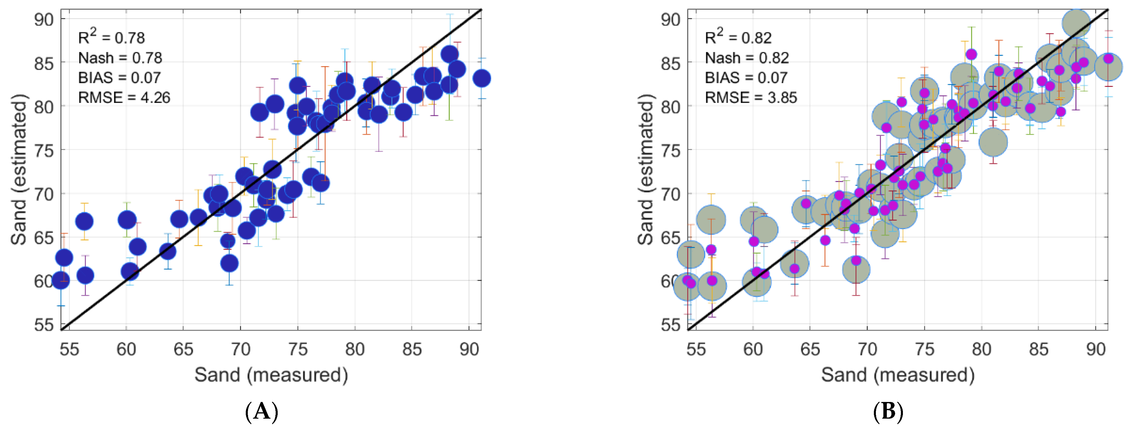
3.3.3. Sand Percentage Estimates

Again, the modeling performance is obviously not similar, with a clear increase in accuracy when the WC is considered in the modeling process (Figure 20B). Two populations of observations are clearly distinguished in Figure 20A (group of samples below 75% sand and above this threshold). These two groups are merged into one when considering WC in the modeling process, resulting in a better estimation quality. This improvement in accuracy is due to the PLSR models training mechanisms related to the subdivision of the database into two classes, as explained above. Nevertheless, in both cases, low percentages of sand are subject to high error rates, even after accounting for WC. This result may confirm the hypothesis raised earlier that the percentages of silt and clay may also strongly influence the spectral response of sand. This could be related to the color component (greyish, yellow, or whitish (light hue) versus brown or brown ochre (dark hue) for sand and silt and clay, respectively).
In fact, the spectral response of the light hue (sand) will of course have a higher magnitude than that of the dark hue (silt and clay), even for high percentages of WC, which can easily be confused with low WC silt and clay spectra (i.e., the confusion area when classifying the database using k-means algorithm; Figure 8). This confusion increases, of course, with lower percentages of sand, as the silt and clay portions are larger. This may explain the inaccuracy of low percentage values (overestimated) even when considering WC (Figure 20B). The error bars are quite similar, with less pronounced bars for the high WC class (grey dots in Figure 20B), highlighting the similarity in the robustness of the sand modeling from the V/NIR spectroscopy data using both approaches. The accuracy of the sand estimates without considering WC was acceptable (R2 = Nash = 0.78, and RMSE = 4.26%) and again was quite similar to the results of the study by Jaconi, Vos and Don [9] where the authors found a R2 = 0.80 of sand for sandy soils. On the other hand, the accuracy achieved when considering the WC effect is relatively higher with R2 = Nash = 0.82, and RMSE = 3.85%. It can be concluded that the WC does affect the sand percentage modeling, but it is not the only parameter that should be considered.

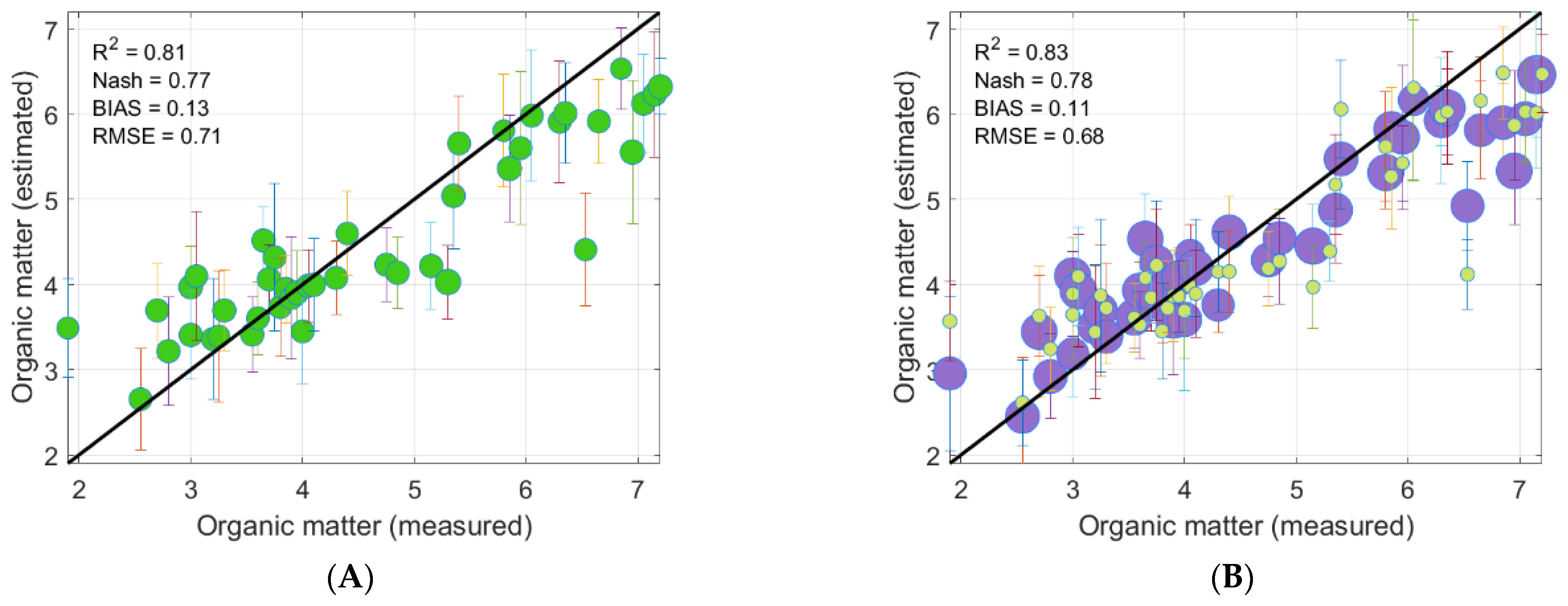
3.3.4. Organic Matter Percentage Estimates

The modeling performance is quite similar in both cases, with a slight increase in accuracy when the WC is considered in the modeling process. This improvement in accuracy is probably related values between 5% and 6%, as they became better distributed around the 1:1 line (Figure 21B). Two populations of observations (Figure 21A) can be distinguished (group of samples below 5.5% sand and above this threshold), but not as clearly as those of silt and sand percentages. However, these two groups are merged into one when considering the WC in the modeling process, resulting in a slightly better estimation quality. As for the silt, low percentage values tend to be overestimated and high percentage values tend to be underestimated in both cases. The error bars are quite similar highlighting the similarity in the robustness of the OM modeling from the V/NIR spectroscopy data using both approaches. It can be concluded that the WC does not much affect the OM percentage modeling. Overall, the accuracies of the OM estimates with or without considering WC were similar and acceptable (R2 = 81, Nash = 0.77, and RMSE = 0.71% and R2 = 83, Nash = 0.78, and RMSE = 0.68%). They were again quite similar to a result conducted by Lazaar et al. [30] where the authors found an R2 = 0.80 and R2 = 0.85 for OM estimated from samples collected from two different sites. It can be concluded that the WC does not affect the OM percentage modeling.

4. Conclusions

The purpose of this work was to compare the modeling performance of soil texture parameters (clay, silt, and sand) and organic matter (OM) with and without considering water content (WC) using visible and near infrared (V/NIR) spectroscopy data. Partial least squares regression was used to train the models in both cases, and the classification and regression tree method was added in the case of considering WC. Evaluation of the models was performed using four statistical indices (R2, Nash criterion (Nash), root-mean-square errors (RMSE), and BIAS) based on the Bootstrap k-fold cross-validation (BKFCV) technique in both cases. The results highlighted the potential of V/NIR spectra to estimate soil particles with sufficient accuracy. For soil texture parameters, the best performance was recorded when considering the WC in the modeling process (R2 up to 0.83, Nash up to 0.83, and RMSE down to 1.00%). Results when WC was not considered in the modeling process were less accurate (R2 up to 0.81, Nash up to 0.78, and RMSE down to 1.07%). For the OM, the best performance was recorded when the WC was taken into account in the modeling process (R2 = 0.83, Nash = 0.78, and RMSE = 0.63%). Results when WC was not considered in the modeling process were less accurate, but were acceptable (R2 = 0.81, Nash = 0.77, and RMSE = 0.71%). Clay and OM were less influenced, while silt and sand were much more influenced by WC. However, it appears that in most cases, whether WC was considered or not, low values tended to be slightly overestimated and high values tended to be slightly underestimated for all soil particles studied. This behavior was more pronounced when WC was not considered, highlighting the importance of taking into account this parameter when modeling soil particles. Nevertheless, the low percentages of sand remained affected by a strong overestimation even when considering WC, leading to the conclusion that sand modeling is also influenced by other soil components, notably the hue. This study highlighted the potential of V/NIR spectroscopy data and the added value of considering WC in the estimation of soil texture parameters and OM. The results showed that WC can, at some level, improve the quality of soil parameter modeling (Table 3), but some of the variance remained unexplained. Incorporating other soil properties (hue, structure, infiltration capacity, nutrient sorption, soil carbon turnover, compaction, etc.) into a deep learning model could further improve the accuracy of soil parameter modeling, especially sand and OM. This kind of tool could be of great help for soil quality monitoring managers, especially in provinces such as Quebec, which covers a very large territory.

Author Contributions

Conceptualization, K.C.; methodology, K.C., A.H., A.N.C. and A.E.A.; validation, A.H. and A.E.A.; formal analysis, K.C., A.H. and A.E.A.; resources, K.C. and A.H.; data curation, A.H.; writing—original draft preparation, A.E.A.; writing—review and editing, K.C., A.H., A.N.C. and A.E.A.; supervision, K.C. and A.N.C.; project administration, K.C.; funding acquisition, K.C. All authors have read and agreed to the published version of the manuscript.

Funding

This research received no external funding.

Data Availability Statement

All data collected, pre-processed, processed, or analyzed during this study are included in this work.

Acknowledgments

The authors would like to thank the Ministry of Agriculture, Fisheries and Food of Québec for providing the soil samples for this study. Our thanks also go to the INRS and the Tunisian government for their funding of the internships.

Conflicts of Interest

The authors declare no conflict of interest.

References

  1. Brabant, P. Activités Humaines et Dégradation des Terres. Collection Atlas Cédéroms. Indicateurs et Méthodes; IRD: Paris, France, 2008. Available online: www.cartographie.ird.fr/degra_PB.html (accessed on 15 May 2022).
  2. Phogat, V.; Tomar, V.; Dahiya, R. Soil physical properties. In Soil Science: An Introduction; Indian Society of Soil Science: New Delhi, India, 2015; pp. 135–171. [Google Scholar]
  3. Benedet, L.; Faria, W.M.; Silva, S.H.G.; Mancini, M.; Demattê, J.A.M.; Guilherme, L.R.G.; Curi, N. Soil texture prediction using portable X-ray fluorescence spectrometry and visible near-infrared diffuse reflectance spectroscopy. Geoderma 2020, 376, 114553. [Google Scholar] [CrossRef]
  4. Ball, D.W. Field Guide to Spectroscopy; SPIE Press: Bellingham, WA, USA, 2006; Volume 8. [Google Scholar]
  5. Pinheiro, É.F.; Ceddia, M.B.; Clingensmith, C.M.; Grunwald, S.; Vasques, G.M. Prediction of soil physical and chemical properties by visible and near-infrared diffuse reflectance spectroscopy in the central Amazon. Remote Sens. 2017, 9, 293. [Google Scholar] [CrossRef] [Green Version]
  6. Kizewski, F.; Liu, Y.T.; Morris, A.; Hesterberg, D. Spectroscopic approaches for phosphorus speciation in soils and other environmental systems. J. Environ. Qual. 2011, 40, 751–766. [Google Scholar] [CrossRef] [PubMed]
  7. Zaady, E.; Karnieli, A.; Shachak, M. Applying a field spectroscopy technique for assessing successional trends of biological soil crusts in a semi-arid environment. J. Arid. Environ. 2007, 70, 463–477. [Google Scholar] [CrossRef]
  8. Hermansen, C.; Knadel, M.; Moldrup, P.; Greve, M.H.; Karup, D.; de Jonge, L.W. Complete soil texture is accurately predicted by visible near-infrared spectroscopy. Soil Sci. Soc. Am. J. 2017, 81, 758–769. [Google Scholar] [CrossRef]
  9. Jaconi, A.; Vos, C.; Don, A. Near infrared spectroscopy as an easy and precise method to estimate soil texture. Geoderma 2019, 337, 906–913. [Google Scholar] [CrossRef]
  10. Villas-Boas, P.R.; Romano, R.A.; de Menezes Franco, M.A.; Ferreira, E.C.; Ferreira, E.J.; Crestana, S.; Milori, D.M.B.P. Laser-induced breakdown spectroscopy to determine soil texture: A fast analytical technique. Geoderma 2016, 263, 195–202. [Google Scholar] [CrossRef] [Green Version]
  11. Rossel, R.V.; Jeon, Y.; Odeh, I.; McBratney, A. Using a legacy soil sample to develop a mid-IR spectral library. Soil Res. 2008, 46, 1–16. [Google Scholar] [CrossRef]
  12. Bach, H.; Mauser, W. Modelling and model verification of the spectral reflectance of soils under varying moisture conditions. In Proceedings of the IGARSS’94-1994 IEEE International Geoscience and Remote Sensing Symposium, Pasadena, CA, USA, 8–12 August 1994; pp. 2354–2356. [Google Scholar]
  13. Somers, B.; Gysels, V.; Verstraeten, W.; Delalieux, S.; Coppin, P. Modelling moisture-induced soil reflectance changes in cultivated sandy soils: A case study in citrus orchards. Eur. J. Soil Sci. 2010, 61, 1091–1105. [Google Scholar] [CrossRef]
  14. Minasny, B.; McBratney, A.B.; Bellon-Maurel, V.; Roger, J.-M.; Gobrecht, A.; Ferrand, L.; Joalland, S. Removing the effect of soil moisture from NIR diffuse reflectance spectra for the prediction of soil organic carbon. Geoderma 2011, 167, 118–124. [Google Scholar] [CrossRef] [Green Version]
  15. Ji, W.; Viscarra Rossel, R.; Shi, Z. Accounting for the effects of water and the environment on proximally sensed vis–NIR soil spectra and their calibrations. Eur. J. Soil Sci. 2015, 66, 555–565. [Google Scholar] [CrossRef]
  16. Group, S.C.W. The Canadian System of Soil Classification; Agriculture and Agri-Food Canada: Ottawa, ON, Canada, 1998; 187p.
  17. Kroetsch, D.; Wang, C. Particle size distribution. Soil Sampl. Methods Anal. 2008, 2, 713–725. [Google Scholar]
  18. Lekshmi, S.; Singh, D.N.; Baghini, M.S. A critical review of soil moisture measurement. Measurement 2014, 54, 92–105. [Google Scholar]
  19. MacQueen, J. Some methods for classification and analysis of multivariate observations. In Proceedings of the Fifth Berkeley Symposium on Mathematical Statistics and Probability, Davis, CA, USA, 1 January 1967; pp. 281–297. [Google Scholar]
  20. Jolliffe, I. Principal component analysis. In Encyclopedia of Statistics in Behavioral Science; John Wiley & Sons, Ltd.: Hoboken, NJ, USA, 2005. [Google Scholar]
  21. Breiman, L.; Friedman, J.; Stone, C.J.; Olshen, R.A. Classification and Regression Trees; CRC Press: Boca Raton, FL, USA, 1984. [Google Scholar]
  22. Song, K.; Li, L.; Wang, Z.; Liu, D.; Zhang, B.; Xu, J.; Du, J.; Li, L.; Li, S.; Wang, Y. Retrieval of total suspended matter (TSM) and chlorophyll-a (Chl-a) concentration from remote-sensing data for drinking water resources. Environ. Monit. Assess. 2012, 184, 1449–1470. [Google Scholar] [CrossRef] [PubMed]
  23. Wold, H. Estimation of principal components and related models by iterative least squares. Multivar. Anal. 1966, 391–420. [Google Scholar]
  24. Wold, S.; Sjöström, M.; Eriksson, L. PLS-regression: A basic tool of chemometrics. Chemom. Intell. Lab. Syst. 2001, 58, 109–130. [Google Scholar] [CrossRef]
  25. Efron, B.; Tibshirani, R.J. An Introduction to the Bootstrap; CRC Press: Boca Raton, FL, USA, 1994. [Google Scholar]
  26. James, G.; Witten, D.; Hastie, T.; Tibshirani, R. An Introduction to Statistical Learning; Springer: Berlin/Heidelberg, Germany, 2013; Volume 112. [Google Scholar]
  27. Nash, J.E.; Sutcliffe, J.V. River flow forecasting through conceptual models part I—A discussion of principles. J. Hydrol. 1970, 10, 282–290. [Google Scholar] [CrossRef]
  28. Hunt, G.R. Spectral signatures of particulate minerals in the visible and near infrared. Geophysics 1977, 42, 501–513. [Google Scholar] [CrossRef] [Green Version]
  29. Yoo, W.; Mayberry, R.; Bae, S.; Singh, K.; Peter He, Q.; Lillard, J.W., Jr. A Study of Effects of MultiCollinearity in the Multivariable Analysis. Int. J. Appl. Sci. Technol. 2014, 4, 9–19. [Google Scholar] [PubMed]
  30. Lazaar, A.; Mouazen, A.M.; El Hammouti, K.; Fullen, M.; Pradhan, B.; Memon, M.S.; Andich, K.; Monir, A. The application of proximal visible and near-infrared spectroscopy to estimate soil organic matter on the Triffa Plain of Morocco. Int. Soil Water Conserv. Res. 2020, 8, 195–204. [Google Scholar] [CrossRef]
Figure 1. Geographic location of the experimental fields. The red, orange, and blue frames are zoomed in on the province of Quebec, Sainte-Catherine-de-la-Jacques-Cartier, and Île d’Orléans (Orleans Island), respectively.
Remotesensing 14 03510 g001
Figure 2. Division of each sample into three replicas.
Remotesensing 14 03510 g002
Figure 3. Flow chart of different soil samples treatments for generating the database.
Remotesensing 14 03510 g003
Figure 4. Ocean Optics’ system set for measuring the reflectance of soil samples.
Remotesensing 14 03510 g004
Figure 5. The k-fold cross-validation algorithm.
Remotesensing 14 03510 g005
Figure 6. The bootstrap k-fold cross-validation algorithm taking into account the influence of WC.
Remotesensing 14 03510 g006
Figure 7. The bootstrap k-fold cross-validation algorithm without taking into account the influence of WC.
Remotesensing 14 03510 g007
Figure 8. Flow chart of the methodological approach.
Remotesensing 14 03510 g008
Figure 9. Visible and near-infrared spectra of the database (A) and visible and near-infrared spectra of the database by intervals (B). WC refers to water content.
Remotesensing 14 03510 g009
Figure 10. Spectra of (A) 12.45% clay (equivalent to 32.99% silt, 54.55% sand, and 4.09% OM) and (B) 4.82% clay (equivalent to 14.22% silt, 80.97% sand, and 4.15% OM) according to the WC.
Remotesensing 14 03510 g010
Figure 11. The results of the k-means classification. Green spectra represent soils with low water content and orange spectra represent soils with high water content.
Remotesensing 14 03510 g011
Figure 12. Correlogram between water content and spectroscopy data.
Remotesensing 14 03510 g012
Figure 13. Results of the principal component analysis combined with the classification and regression tree.
Remotesensing 14 03510 g013
Figure 14. Evaluation of clay percentage modeling for (A) high and (B) low water content.
Remotesensing 14 03510 g014
Figure 15. Evaluation of silt percentage modeling for (A) high and (B) low water content.
Remotesensing 14 03510 g015
Figure 16. Evaluation of sand percentage modeling for (A) high and (B) low water content.
Remotesensing 14 03510 g016
Figure 17. Evaluation of organic matter percentage modeling for (A) high water content and (B) low water content.
Remotesensing 14 03510 g017
Figure 18. Evaluation of clay percentage modeling for (A) without considering and (B) considering water content (combined classes). The green and blue dots represent the high and low water content classes, respectively.
Remotesensing 14 03510 g018
Figure 19. Evaluation of silt percentage modeling for (A) without considering water content and (B) considering water content (combined classes). The green and blue dots represent the high and low water content classes, respectively.
Remotesensing 14 03510 g019
Figure 20. Evaluation of sand percentage modeling for (A) without considering water content and (B) considering water content (combined classes). The grey and pink dots represent the high and low water content classes, respectively.
Remotesensing 14 03510 g020
Figure 21. Evaluation of organic matter percentage modeling for (A) without considering water content and (B) considering water content (combined classes). The purple and green dots represent the high and low water content classes, respectively.
Remotesensing 14 03510 g021
Table 1. Classification and textures of soil samples [16].
Name of the SiteSainte-Catherine de la Jacques-CartierIle d’Orléans (Orleans Island)
Field1212
Soil TypeSandy soilSandy soilLoamy soilGravelly soil
Soil TextureLoamy coarse sandLoamy coarse sandCoarse sandy loamCoarse sandy loam
Soil seriesPont-RougeMorinOrléansSaint-Nicolas
Soil
Taxonomic
Orthic Humo-Ferric PodzolOrthic Humo-Ferric PodzolEluviated Dystric BrunisolOrthic Humo-Ferric Podzol
Table 2. Descriptive analysis for the different soil properties studied.
PropertyMinimumMaximumAverageStandard Deviation
Water content (%)0.0031.378.758.42
Clay content (%)2.7213.237.132.36
Silt content (%)3.4034.2718.547.41
Sand content (%)54.2591.1074.219.07
Organic matter content (%)1.907.204.341.35
Table 3. Summary table of results. The colors red, green, blue, and gray correspond to the evaluation indices of clay, silt, sand and organic matter, respectively.
Without Considering the Influence of Water Content Considering the Influence of Water Content
R2NashBIASRMSER2NashBIASRMSE
0.800.80−0.011.070.830.83−0.031.00
0.740.74−0.043.700.810.80−0.093.22
0.780.780.074.260.820.820.073.85
0.810.770.130.710.830.780.110.68
Publisher’s Note: MDPI stays neutral with regard to jurisdictional claims in published maps and institutional affiliations.

