Abstract
Hyperspectral data has attracted considerable attention in recent years due to its high accuracy in monitoring soil salinization. At present, most existing research focuses on the saline soil in a single area without comparative analysis between regions. The regional differences in the hyperspectral characteristics of saline soil are still unclear. Thus, we chose Golmud in the cold–dry Qaidam Basin (QB–G) and Gaotai–Minghua in the relatively warm–dry Hexi Corridor (HC–GM) as the study areas, and used the deep extreme learning machine (DELM) and sine cosine algorithm–Elman (SCA–Elman) to predict soil salinity, and then selected the most suitable algorithm in these two regions. A total of 79 (QB–G) and 86 (HC–GM) soil samples were collected and tested to obtain their electrical conductivity (EC) and corresponding hyperspectral reflectance (R). We utilized the land surface parameters that affect the soil based on Landsat 8 and digital elevation model (DEM) data, selected the variables using the light gradient boosting machine (LightGBM), and built SCA–Elman and DELM from the hyperspectral reflectance data combined with land surface parameters. The results revealed the following: (1) The soil hyperspectral reflectance in QB–G was higher than that in HC–GM. The soils of QB–G are mainly the chloride type and those of HC–GM mainly belong to the sulfate type, having lower reflectance. (2) The accuracies of some of the SCA–Elman and DELM models in QB–G (the highest MAEv, RMSEv, and were 0.09, 0.12 and 0.75, respectively) were higher than those in HC–GM (the highest MAEv, RMSEv, and were 0.10, 0.14 and 0.73, respectively), which has flatter terrain and less obvious surface changes. The surface parameters in QB–G had higher correlation coefficients with EC due to the regular altitude change and cold–dry climate. (3) Most of the SCA–Elman results (the mean in HC-GM and QB-G were 0.62 and 0.60, respectively) in all areas performed better than the DELM results (the mean in HC–GM and QB–G were 0.51 and 0.49, respectively). Therefore, SCA–Elman was more suitable for the soil salinity prediction in HC–GM and QB–G. This can provide a reference for soil salinization monitoring and model selection in the future.
1. Introduction
Soil salinization is an important land degradation problem that plagues the world and seriously threatens food security. From 1986 to 2016, the area of salinized land increased by more than 100 million hectares [1]. On 21 October 2021, the Food and Agriculture Organization of the United Nations (FAO) released a global map of the saline soil distribution [2]. This map shows that the world’s saline soil covered an area of 833 million hectares and was mainly distributed in the arid and semi-arid areas of Asia, Africa, and Latin America. In arid climate zones, 20–50% of the irrigated soils on all of the continents have an excessively high salt content. Therefore, it is imperative to monitor soil salinization in the future.
To date, many scholars have carried out research using multispectral, hyperspectral, thermal infrared, and microwave techniques to study soil salinization [3,4,5,6]. Among them, hyperspectral remote sensing data have the unique advantage of a continuous band and rich information, but the correlation between the different bands is relatively strong. Accordingly, characteristic bands need to be selected to solve the collinearity problem. The existing variable selection methods primarily include the following: (1) filtering (principal component analysis, correlation coefficient, gray correlation, and chi-square test); (2) embedding (variable selection method based on penalty items or tree models); and (3) encapsulation (generally combined with the multi-objective grey wolf optimizer (MOGWO) [7], whale optimization algorithm (WOA) [8], sine cosine algorithm (SCA) [9], or other heuristic algorithms). Heuristic algorithms can obtain a better solution in a short time and have been widely used in model prediction [10,11,12]. The filtering method is based on statistical principles for variable selection, and has high computational efficiency but low selection accuracy, and is prone to data redundancy. Embedding and encapsulation methods can effectively improve the selection accuracy and reduce the data dimensions [13].
Artificial intelligence methods are widely used in soil salinization research. The concept of artificial intelligence was introduced in 1956. At the end of the 20th century, non-linear machine learning algorithms developed rapidly and were gradually used by many scholars to construct salinity prediction models, and good results were achieved [14,15]. By 2012, deep learning algorithms had gradually become widely used. Deep learning is the further development of machine learning and can be used to mine data and obtain multiple levels of information. Such algorithms have a strong generalization ability and robustness [16]. Zhang et al. [17] used the Cubist, partial least squares regression (PLSR), and extreme learning machine (ELM) models to establish soil salinity models, and showed the Cubist model had the highest accuracy. Wang et al. [18] used a back propagation neural network (BPNN) to estimate the soil salt content in the Aibi Lake Wetland Nature Reserve and achieved good research results with an R2 of 0.95.
In the SCORPAN equation, the soil is related to a set of auxiliary data, such as the climate, living organisms, relief, parent material, time, and location [19]. Many studies have predicted the soil salinity based on these auxiliary data [20,21]. The soil ecosystem is highly complex, and there may be a nonlinear relationship between soil salinity and spectral reflectance. DELM improves the traditional ELM algorithm by adding the number of hidden layers that can process high-dimensional data more efficiently, and introduces regularization coefficients which can prevent the model from over-fitting [22]. Ouyang et al. [23] confirmed that the developed deep ELM model performed better than other evaluated regression models related to analyzing NOx. Many studies have used the SCA algorithm to optimize the weight and threshold of a neural network to improve its performance [24]. However, these algorithms (e.g., DELM, LightGBM, and SCA) have rarely been used in the salinization research area. Therefore, LightGBM, DELM, and SCA–Elman machine learning algorithms were selected for salinity inversion in this study. EC is a parameter that many researchers use to study soil salinity at the local scale [25,26]. The geographic environments of the Qaidam Basin and the Hexi Corridor are quite different, especially regarding their climates and altitudes. However, although the degree of salinization in these two places is serious, related research is lacking; thus, in this study these environments were chosen as the study areas, and comparative analysis was conducted. We used the LightGBM to select the modeling variables, and then predicted the EC of the different study areas based on hyperspectral data combined with the surface parameters of the SCORPAN equation and conducted a comparative analysis.
2. Material and Methods
2.1. Study Area
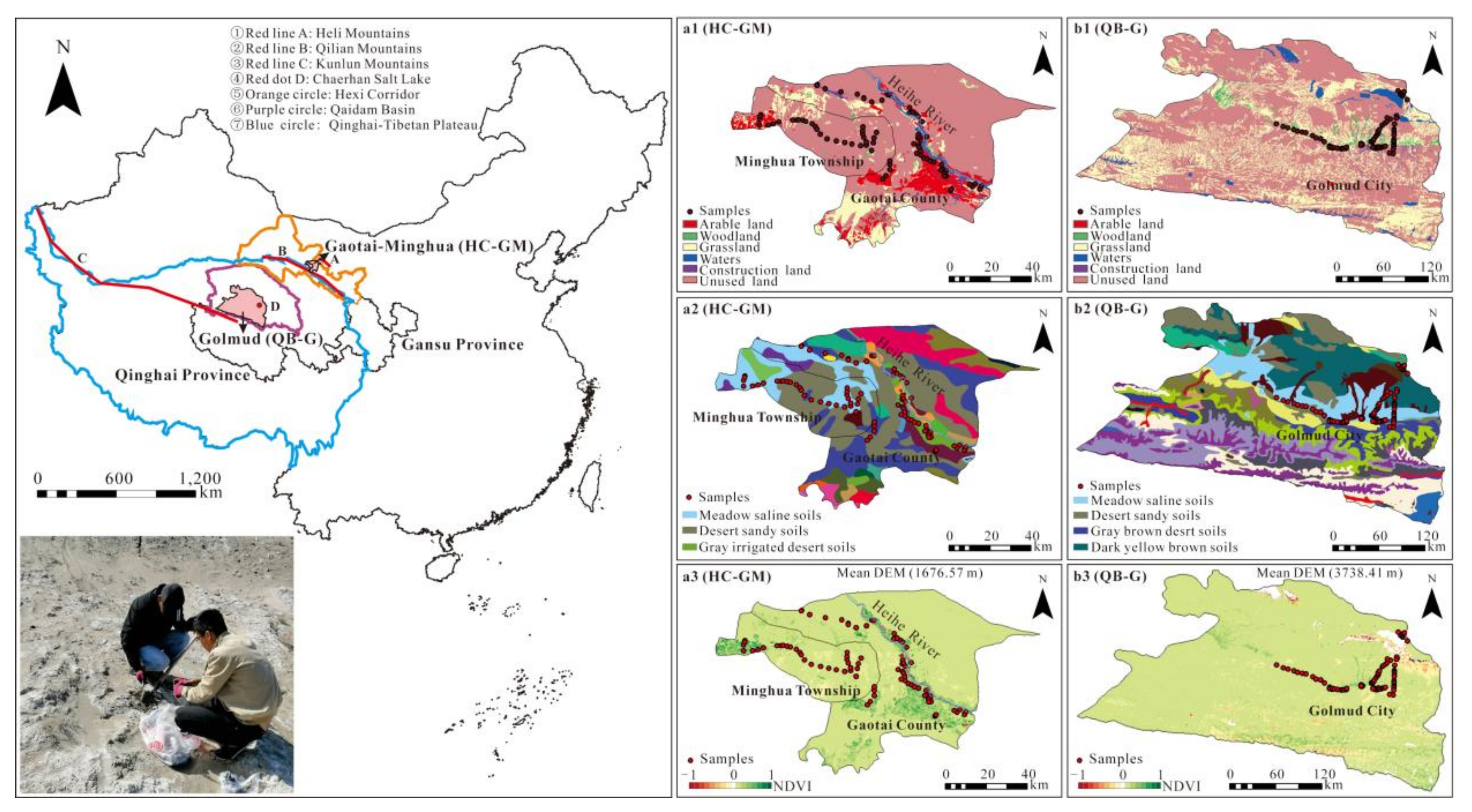
Gaotai County and Minghua Township in Yugur Autonomous County of Sunan are located in the Hexi Corridor (HC–GM) of China (Figure 1). The southern part of HC–GM in the Hexi Corridor contains the Qilian Mountains, and the northern part contains the Heli Mountains. The Heihe River flows through the central flat region of HC–GM. HC–GM has a continental arid climate with little precipitation, and the average annual temperature and precipitation are 8.1 °C and 112.3 mm, respectively. In HC–GM, 23, 2, 3, 5, 3, and 50 samples were collected from arable land, woodland, grassland, waters (e.g., beaches in this study), construction land, and unused land (e.g., sandy land, Gobi, saline–alkali land, marshland, bare land, and other lands), respectively. Among the samples from HC–GM, 21, 23, and 23 samples were categorized as meadow saline soils, desert sandy soils, and gray irrigated desert soils, respectively, and the remaining samples belonged to other soils. The soil type map used the Chinese soil genetic classification system. The normalized difference vegetation index (NDVI) was calculated from Landsat 8.

Figure 1.
Distribution of the samples in HC–GM and QB–G, including their (a1,b1) land use maps (from https://www.resdc.cn/Default.aspx) (accessed on 7 September 2021), (a2,b2) soil type maps (from https://www.resdc.cn/Default.aspx) (accessed on 7 September 2021), (a3,b3) NDVI maps (from https://www.gscloud.cn/) (accessed on 7 September 2021).
The Qaidam Basin is located in the northwestern part of Qinghai Province and the northeastern part of the Qinghai–Tibetan Plateau (Figure 1). It is one of the four major basins in China. The southern part of Golmud in the Qaidam Basin (QB–G) contains the Kunlun Mountains, and the northern part contains the Chaerhan Salt Lake. The landform types in QB–G from south to north include a plateau, a proluvial plain, an alluvial–proluvial plain, an alluvial plain, a salt lake sedimentary plain, and a denudation plain. QB–G has a plateau continental climate, with an average temperature of −6.5 °C in winter and 17.5 °C in summer. This area has a high altitude and a cold climate. In QB–G, 17, 11, 28, and 23 samples were collected from arable land, woodland, grassland, and unused land, respectively. The soil types of 35, 12, 10, and 15 samples were classified as meadow saline soils, desert sandy soils, gray–brown desert soils, and dark yellow–brown soil, respectively, and the remaining samples belonged to other types.
2.2. Datasets
2.2.1. Electrical Conductivity and Eight Major Saline Ions Data
In this study, 79 and 86 samples were collected from QB–G and HC–GM, respectively, based on the accessibility of the areas from September to October 2020 when there was no precipitation to wash the salt away and the evaporation was strong; thus, the salt was exposed at the surface as the water evaporated. We collected samples at a depth of 10 cm below the surface and three replicates at each sample point were collected. The collected soil samples were dried in a ventilated laboratory and then sieved through a 1 mm sieve to test the soil EC and hyperspectral reflectance in the laboratory.
The soil solution was prepared according to a water–soil ratio of 5:1. It was stirred well and left to stand for 1 h. The EC of the filtrate was measured after extraction. In addition, we also measured the eight major saline ions in the soil (, , , , , , , and ).
2.2.2. Hyperspectral Reflectance Data
We used an ASD FieldSpec 4 spectrometer (Analytical Spectral Devices, Boulder, Colorado, USA) with a spectral range of 350–2500 nm to measure the hyperspectral reflectance of soil samples, with a resampling interval of 1 nm. We placed a 70 W halogen lamp that simulates sunlight in a darkroom in the laboratory. A dark-colored vessel with a diameter of 20 cm and a depth of 2 cm was used to hold the soil samples. The distances between the light source and the probe, and between the probe and the soil, were 50 and 10 cm, respectively, and the zenith angle was 15°. Before each measurement, we used a whiteboard for calibration, and then we collected 20 spectral curves from four directions. Finally, we took the average value as the original hyperspectral reflectance of the sample.
2.2.3. Landsat 8 Remote Sensing Data
Due to the availability of Landsat data for the study areas, eight Landsat 8 OLI datasets from 30 August to 7 October 2020 were selected for use in this study to mosaic into an image. The cloud content was less than 10%, and the resolution was 30 m. The path/row values of the eight Landsat 8 OLI images were 134/32, 134/33, 136/34, 136/35, 137/34, 137/35, 138/34, and 138/35. We used ENVI 5.3 to perform the radiometric calibration and atmospheric correction of the Landsat 8 OLI.
2.2.4. Soil and Terrain Influence Factors
Soil is a complex system. The reflectance of soil is also affected by the parent material, climate, vegetation, topography, water, and salt content [27]. The higher the degree of salinization, the lower the vegetation coverage [28]. The smaller the particle size of the soil, the weaker the absorption of the spectrum [29]. In this study, salinity indexes, vegetation indexes, water indexes, terrain attributes, and drought indexes were included as modeling parameters (Table 1, Table 2, Table 3 and Table 4). The terrain attributes were calculated based on the DEM using the System for Automated Geoscientific Analyses–Geographic Information System (SAGA–GIS), and the other parameters were calculated using the Landsat 8 data in ENVI 5.3. Due to the complexity of the UNVI formula, we calculated it in PyCharm Community Edition 2021.2.1.

Table 1.
Salinity indexes required for the model.
Table 2.
Vegetation indexes required for the model.
Table 3.
Water indexes, drought indexes and remote sensing data required for the model.
Table 4.
Terrain attributes required for the model.
2.3. Methods
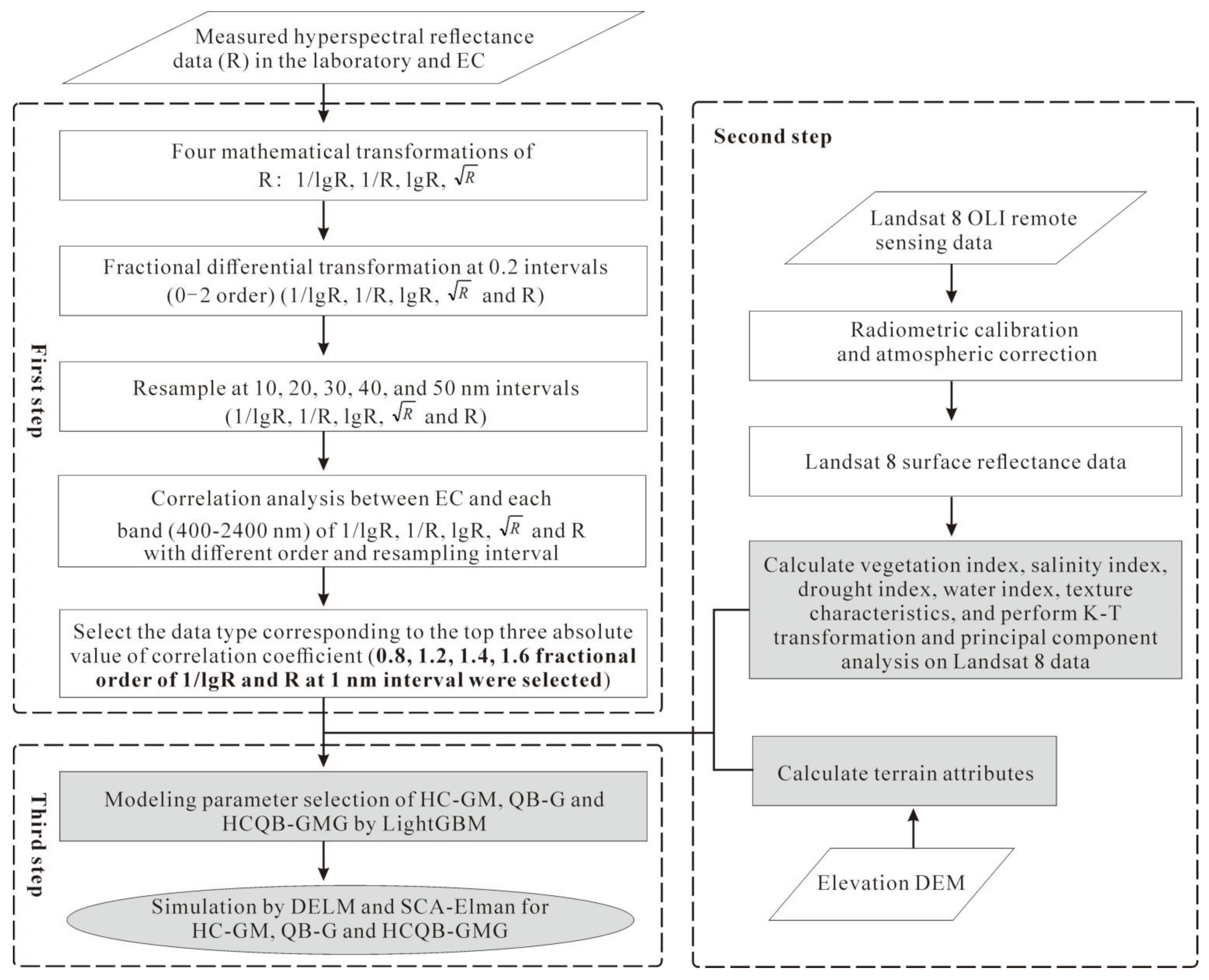
The method used in this study included three main steps (Figure 2). The first step was to select the forms (mathematical form, order, and resampling interval) of the hyperspectral reflectance that corresponded to the top three absolute values of the Pearson correlation coefficient. The hyperspectral reflectances of the selected forms were combined with land surface parameters as the data source of the model. The second step was to calculate the land surface parameters that affect the soil based on Landsat 8 and DEM data. The third step was selecting the variables using LightGBM and modeling using DELM and SCA–Elman for HC–GM, QB–G, and HCQB–GMG.
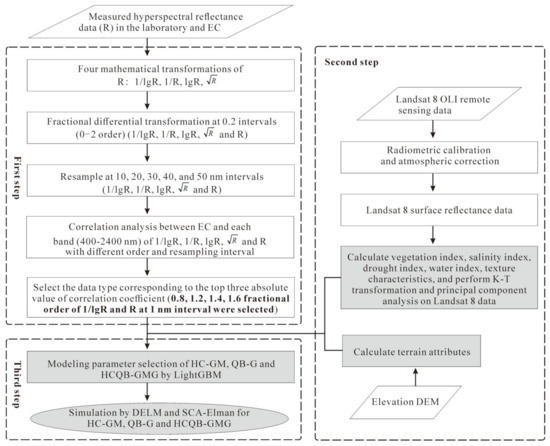
Figure 2.
Technical flowchart of this study.
2.3.1. Hyperspectral Reflectance Data Processing
The band range of hyperspectral data is 350–2500 nm with good band continuity. In this study, first, the 350–399 nm and 2401–2500 nm intervals in the region with low signal-to-noise ratios were deleted, and then Savitzky–Golay filtering of the spectral data was conducted. The Savitzky–Golay smoothing filter is a low-pass filter based on polynomial fitting [53]. The Savitzky–Golay filtering formula is shown in Equation (1).
where is the fitting value of the smoothing noise reduction at the i-point of the spectrum. is the original reflectance at the i-point. is the weight coefficient, and 2m + 1 is the width of the filter window. k is the order of the smoothing polynomial. The number of the left and right size point was 10 and the polynomial order was 2 in the Unscrambler X 10.4.
The 1/lgR, lgR, and 1/R mathematical transformations were performed to eliminate noise interference. Then, we used the fractional differential formula to perform 0–2 order (interval is 0.2 order) differential processing and utilized a resampling method whose intervals included 10, 20, 30, 40, and 50 nm. The Grünwald–Letnikov fractional differential formula is shown in Equation (2).
where α is the order, h is the step size, and t and a are the upper and lower limits of the differential. In the Gamma function, [54,55]. These processes were implemented in MATLAB R2018b.
2.3.2. Variable Selection and Inversion of EC
In this study, the Kennard–Stone algorithm was used to divide the soil samples. The calibration dataset consisted of 2/3 of the data, and the validation dataset consisted of the other 1/3 of the data. There were 57 samples in the calibration dataset and 29 samples in the validation dataset, for a total of 86 soil samples in HC–GM. Among the 79 samples in QB–G, the calibration dataset and validation dataset consisted of 53 and 26 samples, respectively. Among the 165 samples in HCQB–GMG, the calibration dataset and validation dataset contained 110 and 55 samples, respectively.
- (1)
- LightGBM
The LightGBM is an ensemble learning algorithm. An ensemble learning algorithm integrates the prediction results of multiple base learners to improve the generalization ability and robustness of the base learners [56]. The existing ensemble learning methods include serialization methods (e.g., the boosting and LightGBM) and parallelization methods (e.g., bagging and random forest). The LightGBM measures the importance of variable i in a single tree by calculating the reduced loss value of variable i after splitting. The variables with importance values greater than 0 were used in the model in this study. The LightGBM was implemented using the machine learning library (Sklearn) in Python3.7.
- (2)
- DELM
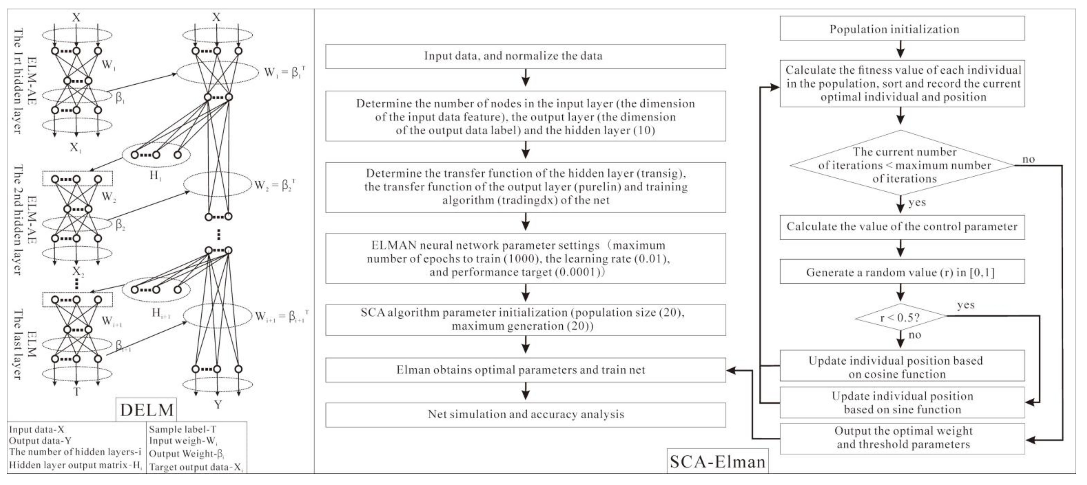
The extreme learning machine (ELM) was developed in 2004 [57]. Wang et al. [58] provided the code for the ELM in their book. The DELM uses multiple extreme learning machine–auto encoders (ELM–AE) to perform unsupervised training (Figure 3). The DELM is initialized based on the output weights of the different ELMs. Therefore, the DELM is also called the multi-layer extreme learning machine (ML–ELM). The deep ELM method both significantly improves the network training time relative to a single ELM and can improve the classification accuracy [59]. Other studies have shown that DELM’s performance is significantly better than that of principal components regression, partial least squares regression, and neural networks [23]. The activation function in this study was the sigmoid function, and the regularization coefficient was introduced in the solution of the weight coefficient to improve the generalization ability of the model. In this study, the DELM model was built in MATLAB R2018b.
- (3)
- SCA–Elman
The Elman model was proposed by J. L. Elman in 1990. It mainly consists of an input layer, hidden layer, inheritance layer, and output layer. Compared with the BP neural network, it has one more inheritance layer, which is beneficial to improving the global stability of the network. Wang et al. [58] provided the code for the Elman model in their book. The SCA is a stochastic optimization algorithm proposed by Seyedali Mirjalili in 2016, and he provided download link (http://www.alimirjalili.com/SCA.html) (accessed on 1 September 2021) for the code in his paper [9]. SCA uses a mathematical model based on sine and cosine to find the optimal solution, and can effectively converge to the global optimal solution. Liu et al. [60] optimized the weights and thresholds of BPNN through particle swarm optimization (PSO), which effectively prevents the training from falling into the local optimum. In the learning process of Pi–Sigma artificial neural networks (PS–ANNs), a position of SCA consists of weight and bias values of the PS–ANNs, and the use of the SCA method in the training of PS–ANNs produces better results than the use of many other artificial intelligence optimization algorithms [24]. Similarly, SCA–Elman used the SCA to optimize the weights and threshold parameters of the Elman model. In this study, SCA–Elman was constructed in MATLAB R2018b.

Figure 3.
Model structure of DELM and SCA–Elman.
Figure 3.
Model structure of DELM and SCA–Elman.
2.3.3. Model Verification
The RMSE, coefficient of determination (R2), and mean absolute error (MAE) were used to verify the model’s ability to predict the EC. The larger the R2, the more stable the model. The smaller the RMSE, the higher the accuracy of the model. The range of MAE is [0, +∞). An MAE of 0 means that the predicted value is basically the same as the true value. As the error increases, the MAE also increases [61].
3. Results
3.1. Descriptive Statistics of the EC and Chemistry Types of the Soil Samples
The mean, SD, and CV of the values corresponding to EC for all of the samples in HC–GM, QB–G, and HCQB–GMG were between those of the calibration dataset and the validation dataset (Table 5), indicating that the quality of the selected samples was good. The CVs of the EC for the samples from HC–GM, QB–G, and HCQB–GMG were all greater than 1, indicating a large degree of variation. The CV for HC–GM was greater than that for QB–G.
Table 5.
Statistical characteristics of the EC of the soil samples from the different areas.
3.2. Hyperspectral Reflectance Curve of Soil Samples
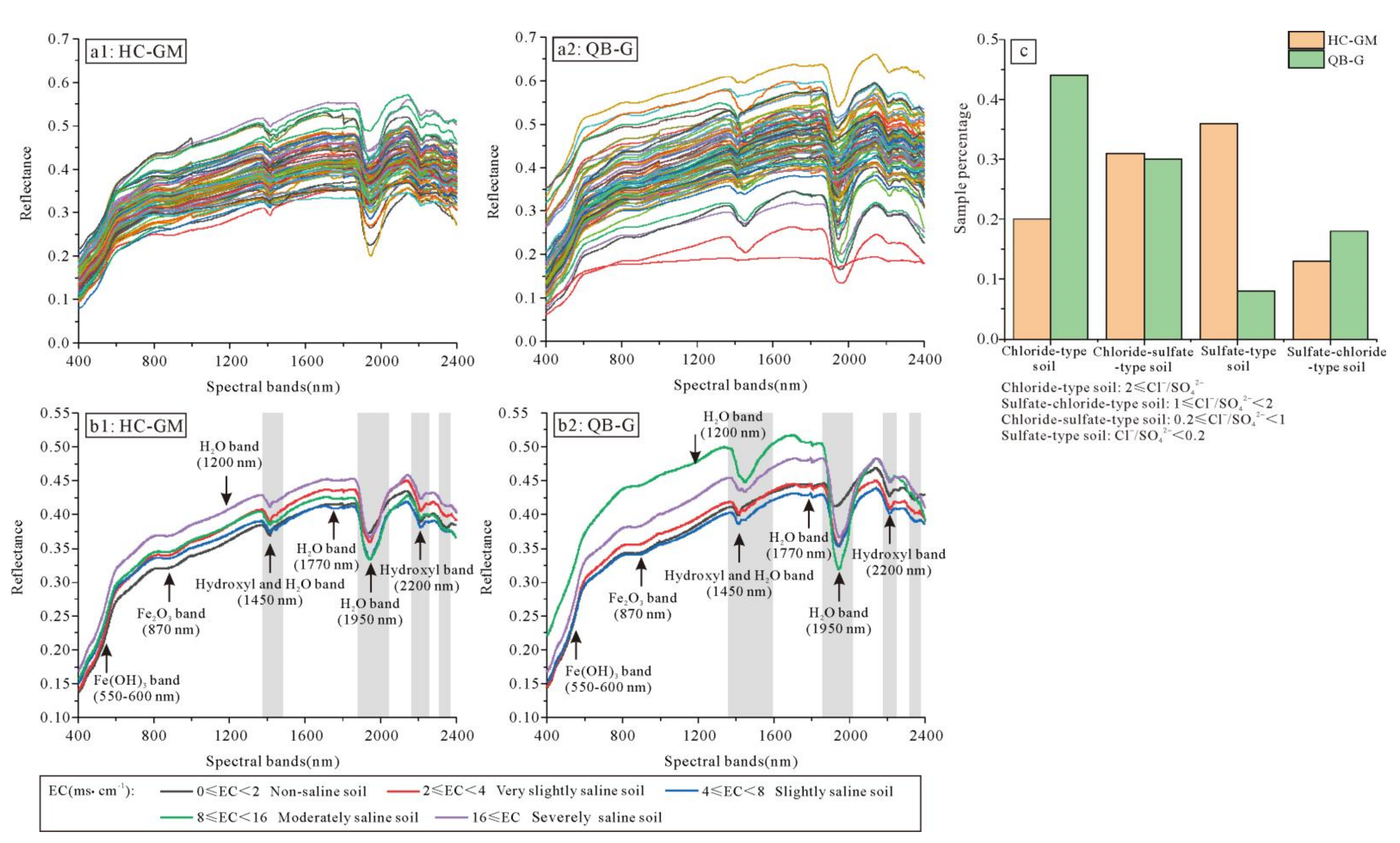
Based on the soil salinity classification standard and the actual situation in the study area, we classified the soil samples as non-saline soil, very slightly saline soil, slightly saline soil, moderately saline soil, and severely saline soil [62] (Figure 4). The slope of the hyperspectral curve for HC–GM and QB–G increased rapidly at 400–600 nm, remained stable at 600–1800 nm with wide and shallower troughs, and gradually decreased at 2000–2400 nm (Figure 4). This revealed that the hyperspectral reflectance curve for HC–GM and QB–G have obvious wave type characteristics [63]. The hyperspectral reflectance of QB–G’s severely saline soil and moderately saline soil was significantly higher than those of the other soils, and the hyperspectral reflectance values of HC–GM samples were directly proportional to their EC. Hygroscopic water refers to the water still contained in the soil after the fresh soil has been dried for 1 week and stabilized under ventilated conditions. The higher the salt content, the greater the moisture content [64]. The soil samples in this study were naturally air dried indoors, so the reflectance of the severely saline soil from QB–G was not the highest. However, this phenomenon was not observed for HC–GM samples, which may be due to their lower salt contents. The shape of soil reflectance curves was affected by the strong water absorption bands at 1450 and 1950 nm, and occasionally weaker water absorption bands at 1200 and 1770 nm in HC–GM and QB–G [65]. An absorption band at 2200 nm was influenced by the vibrational mode of the hydroxyl ion in HC–GM and QB–G [66]. Hydroxyl ion absorption also occurs at 1450 nm, the same as the case of water absorption. Weak absorption bands at 1200 and 1770 nm correspond to the absorption bands observed in transmission spectra of relatively thick water films [67]. Bands at 1450 and 1950 nm were sharp in HC–GM, and the water molecules were located in well-defined, ordered sites; on the contrary, the relatively broader bands at 1450 and 1950 nm in QB–G indicated the water molecules were in relatively unordered sites, probably as water films on soil particle surfaces [66]. The 2200 nm hydroxyl absorption band could be seen in samples of HC–GM and QB–G. The organic-affected form exhibits a concave shape from 500 to 750 nm with a convex shape from 750 to 1300 nm [68], which showed that the spectral curves in HC–GM and QB–G belonged to the organic-affected form. Karmanov [69] found that the reflection intensity of iron hydroxides containing little water and having a dark brown–red color increased most strongly in the wave interval from 550 to 600 nm, which was same as the curve in HC–GM and QB–G. The curve in the study areas was distinguished by an iron absorption band at around 870 nm [66].
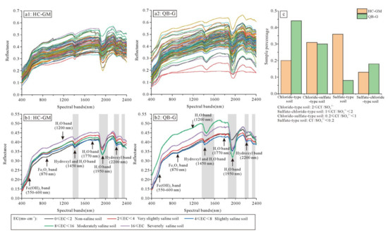
Figure 4.
Hyperspectral reflectance curves of all of the soil samples (a1,a2), curve corresponding to different EC (b1,b2) and the chemical types of the soil samples measured in the laboratory (c).
Based on the soil classification scheme [70], 20%, 13%, 31%, and 36% of all samples from HC–GM and 44%, 18%, 30%, and 8% of all samples from QB–G were classified as chloride-type, sulfate-chloride-type, chloride-sulfate-type, and sulfate-type soils, respectively (Figure 4). Thus, the samples from HC–GM and QB–G were mainly sulfate type and chloride type, respectively. The soil chemicals in the central and southern parts of the Qaidam Basin are mainly NaCI and KCl [71], whereas those in the Hexi Corridor are dominated by sulfate and chloride–sulfate [72], which was consistent with the contents of the eight major saline ions measured in this study. Moreover, NaCl and KCl have weak absorption from the visible to thermal infrared bands, and the average reflectivity of NaCl is higher than that of NaSO4 [64,73,74]. Therefore, the reflectance of the soil in QB–G was generally higher than that in HC–GM.
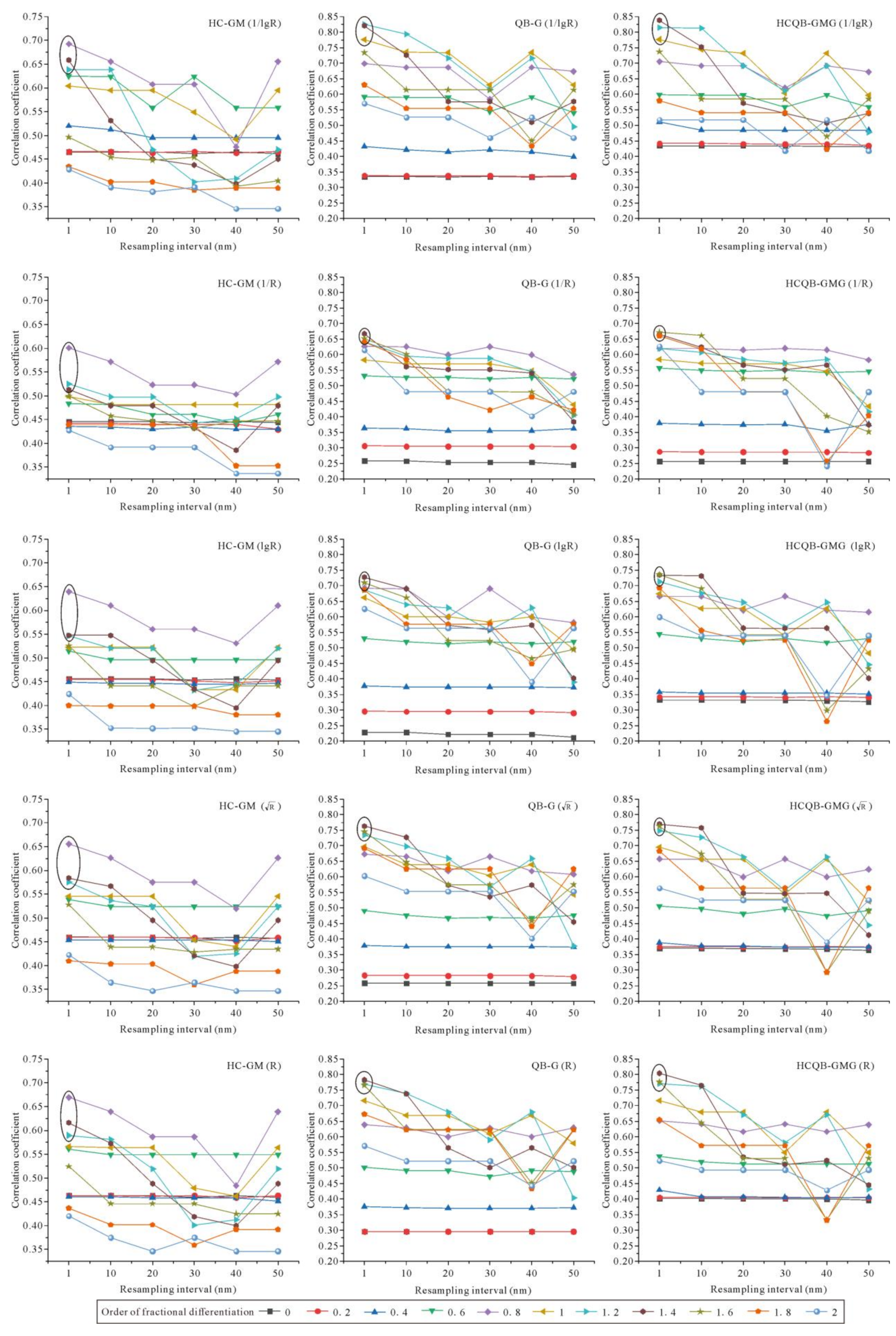
3.3. Correlation between EC and Different Forms of Hyperspectral Reflectance Data
In this study, the correlation coefficients between the EC and each band (400–2400 nm) of the five forms (R, 1/lgR, 1/R, lgR, and ) of hyperspectral reflectance in the 0–2 order at different resampling intervals were calculated. Obviously, the absolute value of the correlation coefficient when the resampling interval was 1 nm was significantly higher. The correlation coefficients of 1/lgR and R were better than those of 1/R, lgR, and for HC–GM, QB–G, and HCQB–GMG (Figure 5). The order of hyperspectral reflectance of the five forms in all study areas corresponding to the top three absolute values of the correlation coefficients was 0.8, 1.2, 1.4, and 1.6. Based on this, we selected 1/lgR and R of orders 0.8, 1.2, 1.4, and 1.6 for the modeling when the band interval was 1 nm.
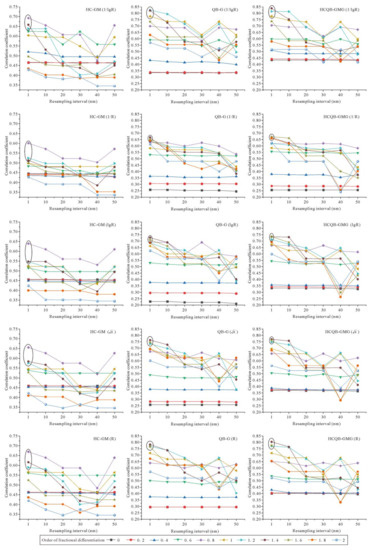
Figure 5.
The absolute value of the correlation coefficient between EC and hyperspectral reflectance with different resampling intervals and orders, and the circles denote the fractional order corresponding to the top three absolute values of the correlation coefficients.
3.4. Simulation of Soil EC Using DELM and SCA–Elman
3.4.1. Modeling Results of DELM and SCA–Elman
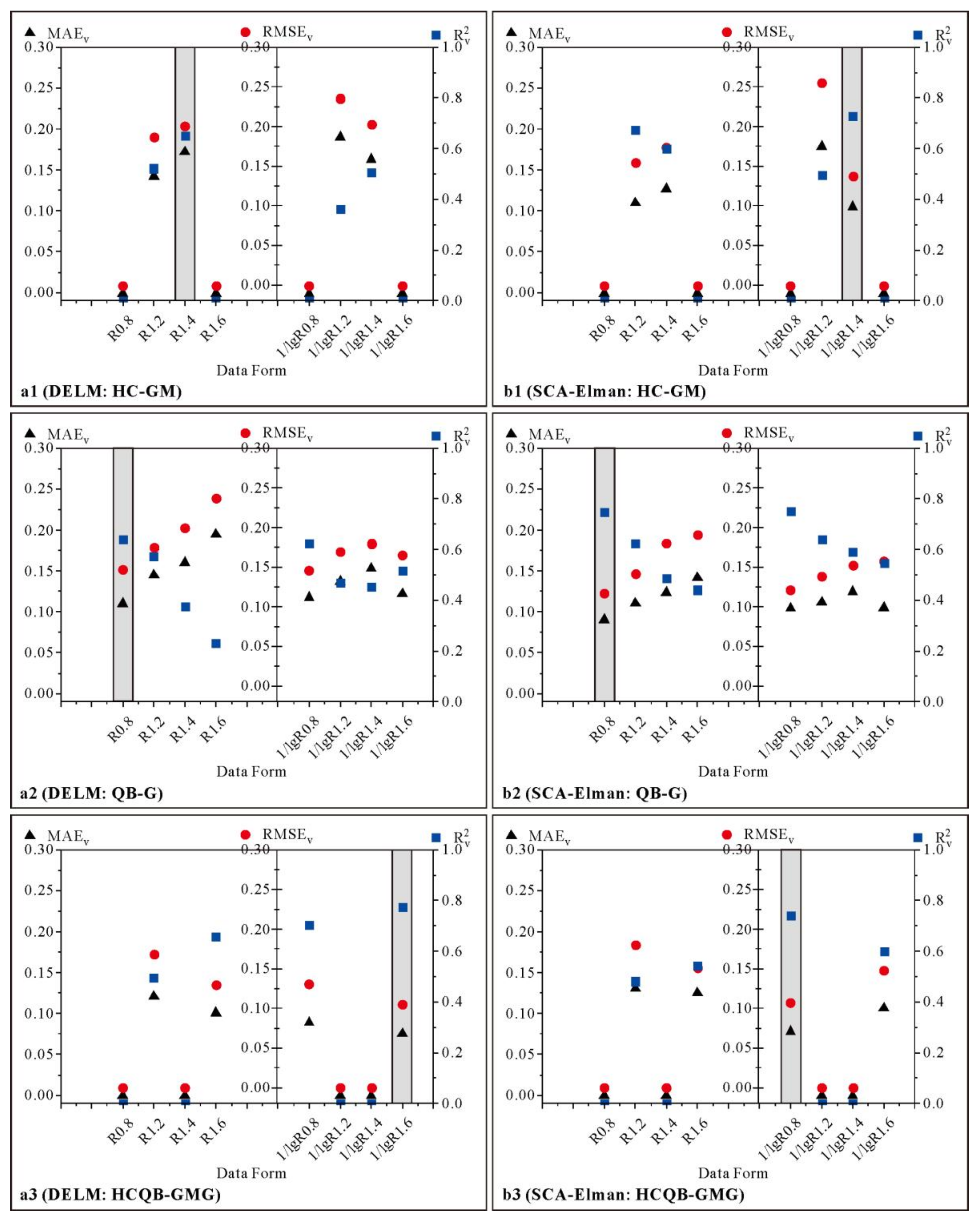
The MAEv, RMSEv, and of the best model among all of the SCA–Elman models in HC–GM were 0.10, 0.14, and 0.73, respectively, which were better than those of DELM for HC–GM. The model with the highest accuracy for QB–G was SCA–Elman whose MAEv, RMSEv, and were 0.09, 0.12 and 0.75, respectively. The best model from all of the models in HC–GM, QB–G and HCQB–GMG was DELM because its multiple hidden layers were more suitable for handling large samples in HCQB–GMG (MAEv = 0.08, RMSEv = 0.11, = 0.77), and whose accuracy was slightly higher than that of SCA–Elman (Figure 6). The accuracy of SCA–Elman for HC–GM and QB–G was basically higher than that of the DELM, but the accuracy of DELM for HCQB–GMG was slightly higher than that of SCA–Elman. Therefore, SCA–Elman is more suitable for salinity prediction in the study areas.
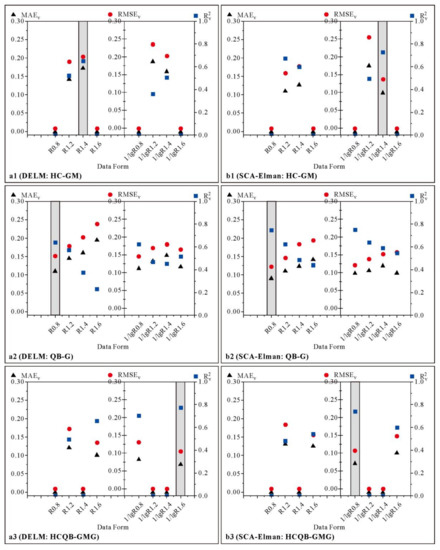
Figure 6.
The modeling results of the validation dataset of the DELM for (a1) HC–GM, (a2) QB–G, and (a3) HCQB–GMG and SCA–Elman for (b1) HC–GM, (b2) QB–G, and (b3) HCQB–GMG with different data sources (the values of MAE and RMSE were processed with min–max normalization). The gray column indicates the optimal model’s accuracy.
3.4.2. Modeling Results for Different Data Forms and Different Regions
For HC–GM, the order with the highest accuracy of DELM was 1.4 for R, whereas that of SCA–Elman was 1.4 for 1/lgR (Figure 6). For QB–G, the order with the highest accuracy of DELM and SCA–Elman was 0.8 for R. For HCQB–GMG, the order with the highest accuracy of DELM was 1.6 for 1/lgR, whereas that of SCA–Elman was 0.8 for 1/lgR. Overall, the accuracies for the 1/lgR with different fractional orders were slightly higher than those of R, and its over-fitting and under-fitting phenomena appeared less frequently than those of R. The accuracies of most of the models with data sources on the order of 0.8 were basically better than those with orders of 1.2, 1.4, and 1.6, indicating that the fractional differential transformation and mathematical transformation improved the accuracy of the model.
By counting the average values of the accuracy indicators of the different models for HC–GM, QB–G, and HCQB–GMG, we found that the accuracy of all of the SCA–Elman and DELM models for HC–GM and QB–G was similar (Table 6). In HC-GM and QB-G, the accuracy of SCA-Elman was slightly higher than DELM, which indicated that SCA-Elman was more suitable for salinity prediction in these two study areas.
Table 6.
The mean values of all of the model validation indicators for the different regions (the values of MAE and RMSE were the values after min–max normalization).
3.5. Correlation between Different Surface Parameters and EC
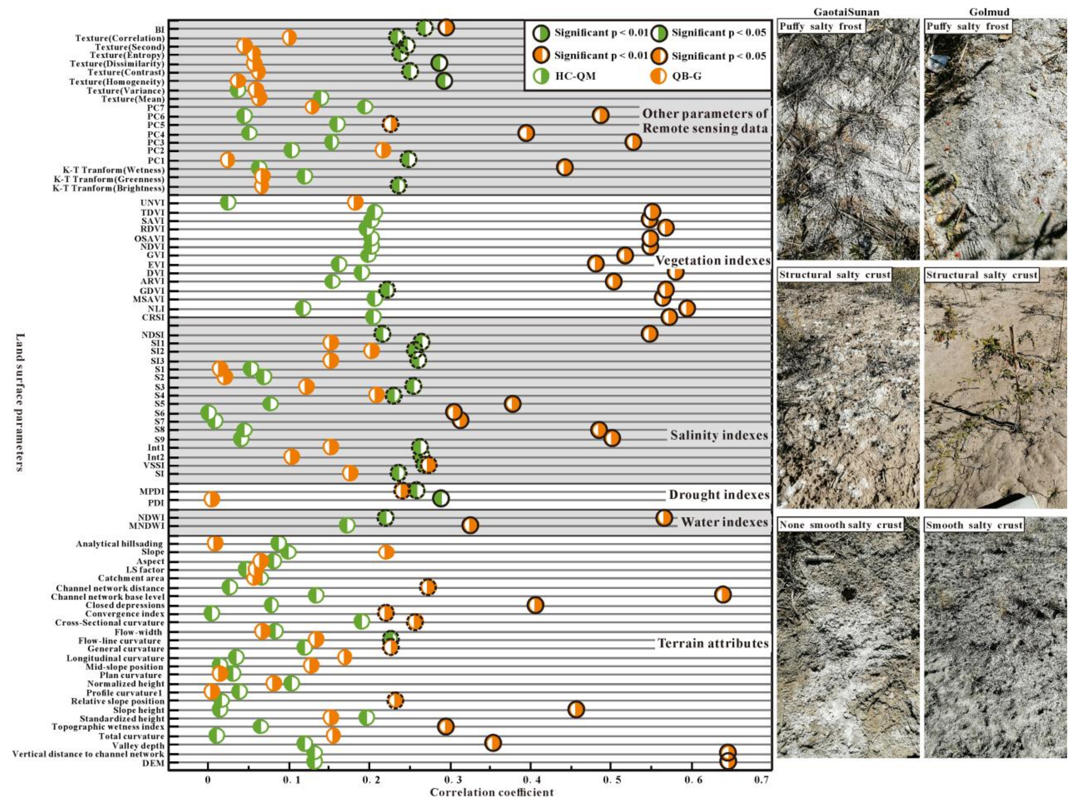
All vegetation indexes in QB–G passed the significance test, whereas in HC–GM only GDVI passed the significance test (Figure 7). GDVI has higher sensitivity than NDVI, SAVI, EVI, and SARVI under low vegetation coverage [37]. Most of the salinity indexes in HC–GM passed the significance test, and the number was slightly greater than that of QB–G. The MPDI and NDWI of QB–G and HC–GM passed the significance test. Among all the terrain attributes in HC–GM, only flow-line curvature passed the significance test, whereas many terrain attributes in QB–G showed a high correlation with EC. Other parameters of remote sensing data that passed the significance test in QB–G were wetness of Kauth–Thomas (K–T) transformation, PC3–6, and BI. Brightness of K–T transformation, PC1, texture (homogeneity, contrast, dissimilarity, entropy, second, correlation), and BI passed the significance test in HC–GM.

Figure 7.
The absolute value of Pearson correlation coefficients between the land surface parameters and soil EC, and the field photos of HC–GM and QB–G.
4. Discussion
4.1. Analysis of Correlation between Different Surface Parameters and EC
The correlations between the vegetation indexes and the EC in the two regions were relatively high, but they were higher in QB–G than in HC–GM. Generally, the higher the degree of salinization, the lower the vegetation coverage [75]. The EC of most of the samples from QB–G was higher, and was coupled with the cold–dry climate of this area. This had a harmful impact on the vegetation, which mainly comprises salt-sensitive plants, and enhanced the sensitivity of the vegetation to salinity. The Heihe River Basin in the Hexi Corridor is becoming warmer and wetter [76,77], which enhances the salt tolerance of vegetation, especially halophytes. NDVI proved to be an ambiguous indicator of soil salinization because it is also related to biomass, leaf area, plant cover, and nitrogen and chlorophyll content, and its sensitivity differs among species [78]. Zhang et al. found that most vegetation indexes have a weak relationship with soil salinity (mean R2 = 0.28) [79]. In the study of Wang et al., NDVI, RVI, GDVI, SAVI, and EVI failed the significance test (p < 0.05) with the soil EC [21]. In addition, most of the samples (50 of 86 samples) on HC–GM were distributed on unused land with low vegetation coverage, which was proved by the NDVI map of Figure 1, and most vegetation indexes are not applicable to this land use type. However, there were fewer samples (23 of 79 samples) of unused land in QB–G.
The climates of HC–GM and QB–G are dry. Evaporation is relatively strong in high salinity regions, and the surface is relatively dry [80]. PDI is more suitable for bare soil. Ghulam et al. introduced the vegetation coverage factor into the PDI and proposed the MPDI [52]. In this study, some samples were distributed in grassland and arable land with vegetation. HC–GM is located in an oasis in the middle reaches of the Heihe River, so its terrain is flat. The altitude in QB–G gradually decreases from the southern mountains to the salt lake in the center of the Qaidam Basin, and the vegetation cover decreases with decreasing distance from the salt lake. Akramkhanov et al. [81] found that most of the terrain attributes had a low correlation with soil salinity because the study area was very flat, which was similar to HC–GM. However, other research proved that combining satellite data with DEM data to study soil salinity will make the results more effective and improve accuracy [6], when the surface terrain is similar to that of QB–G.
In another study, we found that PC2 and PC3 attained the highest correlation with the soil EC and there was a statistically significant correlation between the measured soil salinity and the wetness of K–T transformation [21]. Wang found that the wetness of K–T transformation and the salinity index were important [82], which was consistent with the research in this article. QB–G and HC–CS have many salinity indexes that pass the 0.05 and 0.01 significance tests, and their number was higher than that of other indexes. The correlation between the texture and EC was higher in HC–GM than that in QB–G. The mean EC of HC–GM (8.06) was far below that of QB–G (30.92). There were obvious salty crusts in QB–G. In the field investigation, we found that the soil of QB–G has a puffy salty frost and structural crust due to irrigation in the cultivated land, and a smooth salty crust in the grassland, which had higher reflectance than the slight and non-saline soil without crust or salty frost [75,83,84]; this indicated that its surface conditions were relatively uniform (Figure 7). The soil type of Figure 1 shows that most of the samples in HC–GM were evenly distributed in different soil types, whereas many samples (35 in 79) from QB–G were distributed in meadow saline soils. Thus, the texture in QB–G had a weak correlation with EC. Because BI carries the brightness information of the image, BI is positively correlated with EC, and the area with high BI corresponds to the high EC in the image [85]. The BI of QB–G and HC–CS were both significantly correlated with EC. According to remote sensing images, the high values of PC are mainly distributed in high brightness areas [86]. PC3 and EC were highly correlated in QB–G, and PC1 and EC were significantly correlated in HC–CS, because of the high amount of information of the first three components of the PCA. Metternicht and Zinck [75] proved that PCA of remote sensing images was a useful method to distinguish saline soils. In the Ardakan region of Yazd Province in central Iran, the most important of various auxiliary data for EC prediction were PC1–3 and terrain attributes [87].
The indexes that passed the significance test in HC–GM (PDI, MPDI, VSSI, Int2, SI2, NDSI, BI, GDVI) and QB–G (MPDI, MSAVI, CRSI, NLI, VSSI, S5, NDSI, BI, GDVI, DVI, EVI, GVI, and NDVI) were all calculated with the fourth (red band) and fifth bands (near infrared band) of Landsat 8. Other studies have shown that the red and near-infrared bands contain more soil salinity information [88,89]. Over-fitting and under-fitting problems indicate that the generalization ability of the model is weak [90]. HCQB–GMG ( = 0.77) had the highest accuracy among all of the models for all of the areas. It was even slightly higher than that of SCA–Elman ( = 0.74), which shows that the two areas have similarities in terms of dry climate. However, DELM and SCA–Elman had serious over-fitting problems for HC–GM and higher accuracies for QB–G. The changes in the surface environment, especially the altitude and vegetation, are subject to more obvious natural laws in QB–G, whereas HC–GM is located in the flatter oasis of the Heihe River with a single surface environment. Some studies achieved similar results [82,91,92,93] (Table 7), including those of Peng et al. [91] and Wang et al. [82], whose study areas comprised flat alluvial fans and oases, respectively. Thus, most of the land surface parameters had higher correlation coefficients in QB–G than in HC–GM. This resulted in the lower accuracies of the models for HC–GM. In addition, this may be due to the relatively lower matching between the sub-samples and pixels of Landsat 8 in HC–GM than that in QB–G.
Table 7.
The absolute value of correlation coefficients between soil EC and land surface parameters of different studies.
4.2. Advantages of Hyperspectral Data and Fractional Differential Transformation
Hyperspectral data contain abundant spectral information [94], but they are prone to data redundancy, so it is necessary to select characteristic variables. The image filtering method based on the fractional order is better than that based on the integer order, which can significantly enhance image edges and avoid large noise [95]. The 0.8, 1.2, 1.4, and 1.6 order differential transformations in this study significantly enhanced the correlation between the hyperspectral reflectance and the EC. The models based on these four fractional orders performed better than those based on the original spectral reflectance in HC–GM, QB–G, and HCQB–GMG. Other scholars have reached similar conclusions. Hong et al. [96] reported that the partial least squares support vector machine (PLS–SVM) based on an order of 1.25 achieved the best performance.
4.3. Analysis of the Different Machine Learning Algorithms
At present, many improved algorithms for ELM have been developed [97,98,99]. In this study, the introduction of a regularization coefficient improved the generalization ability of the model [23]. Thus, the simulation accuracy of the DELM for HCQB–GMG was the highest among all of the models for all of the areas. ELM has a single hidden layer, and DELM uses a multi-hidden layer structure to increase the applicability for large samples. The SCA algorithm is characterized by a simple structure, fast convergence speed, high exploratory power, and local optimal avoidance. In this study, the SCA algorithm was used to optimize the weight and threshold parameters of the Elman net. The simulation accuracies of most of the SCA–Elman results for HC–GM and QB–G were better than those of the DELM. Even for HCQB–GMG, the accuracy of SCA–Elman was only slightly lower than that of DELM. Nabiollahi et al. reported similar results using three optimization algorithms (i.e., particle swarm optimization (PSO), genetic algorithm (GA), and bat algorithm (BAT)) to compare the hybridized RF and the standard RF, and concluded that the PSO–RF performed best [100].
Taghadosi et al. extracted features from the radar intensity images and texture analysis of Sentinel-1 data and established soil salinization monitoring models [101]. Zhang et al. extracted normalized backscatter coefficient, entropy, alpha, anisotropy, and other radar indexes from Sentinel-1 dual-polarized data for salinization inversion [102]. Two gamma–nought backscattering coefficients and various textures features were included in the soil salinity mapping in the study of Hoa et al. [103], all of which achieved good results. Shi et al. conducted a meta-analysis of salinization prediction research, selected 57 articles, and found that models using radar data such as Sentinel-1 outperformed Landsat, whereas models using hyperspectral satellite data such as HJ-1 and EO-1 Hyperion performed similarly to Landsat [104]. Therefore, radar data can be used for soil salinization prediction modeling and regional mapping in the future.
5. Conclusions
Soil salinization is a serious land degradation problem in arid and semi-arid regions of the world. Hyperspectral data has the advantages of high spectral resolution, continuous bands, and rich information, which are beneficial to the modeling of this research. In this study, QB–G in the Qaidam Basin and HC–GM in the Hexi Corridor were chosen, combined with machine learning methods to monitor the difference in the salinization in these two areas. The 1/lgR mathematical transformation was found to improve the correlation between the hyperspectral reflectance and the EC. In addition, the correlations between the hyperspectral reflectance of the 0.8, 1.2, 1.4, and 1.6 orders and the EC were significantly better. The soils of QB–G mainly belonged to the chloride type, whereas sulfate-type soils predominated in HC-GM. The reflectance of the chloride-type soil was higher than that of sulfate-type soil. The results of most of the SCA–Elman modeling for HC–GM and QB–G were better than those of DELM, indicating that SCA–Elman was more suitable for monitoring salinity in these areas. The accuracy of the salinization monitoring model for QB–G was higher than that for HC–GM. The topography of the oasis in HC–GM is flatter with less obvious surface changes. The topography and vegetation in QB–G exhibit regular changes as the altitude decreases from the south to the center of Qaidam Basin, and its cold–dry climate weakens the tolerance of the vegetation to salt, which results in a higher correlation with the EC. However, DELM for HCQB–GMG had the highest accuracy for HC–GM, QB–G, and HCQB–GMG, which shows that HC–GM and QB–G are similar in terms of their dry climates. This study can provide a valuable reference for salinity prediction and regional development.
Author Contributions
X.J. and P.G. participated in collecting samples in the field sampling. X.X., H.D., J.L., C.H. helped design the sampling in the field. X.J. completed the experiment in the laboratory, data analysis and paper writing. X.X. and H.D. revised the manuscript. All authors have read and agreed to the published version of the manuscript.
Funding
This research was funded by the Special Fund Project for the Central Government to Guide the Development of Local Science and Technology of China and the National Key Research and Development Program of China (2017YFE0119100).
Data Availability Statement
Publicly available datasets were used in this study. Land use maps is from https://www.resdc.cn/Default.aspx (accessed on 7 September 2021); Soil type maps is from https://www.resdc.cn/Default.aspx (accessed on 7 September 2021); NDVI maps is from https://www.gscloud.cn/ (accessed on 7 September 2021); The code of SCA algorithm is from http://www.alimirjalili.com/SCA.html (accessed on 1 September 2021).
Conflicts of Interest
The authors declare no conflict of interest.
References
- Ivushkin, K.; Bartholomeus, H.; Bregt, A.K.; Pulatov, A.; Kempen, B.; de Sousa, L. Global mapping of soil salinity change. Remote Sens. Environ. 2019, 231, 111260. [Google Scholar] [CrossRef]
- FAO. Status of the world’s soil resources. Agric. Compr. Dev. China 2021, 10, 64. [Google Scholar]
- Csillag, F.; Pasztor, L.; Biehl, L.L. Spectral band selection for the characterization of salinity status of soils. Remote Sens. Environ. 1993, 43, 231–242. [Google Scholar] [CrossRef]
- Dwivedi, R.S.; Sreenivas, K. Image transforms as a tool for the study of soil salinity and alkalinity dynamics. Int. J. Remote Sens. 1998, 19, 605–619. [Google Scholar] [CrossRef]
- Muller, S.J.; van Niekerk, A. Identification of WorldView-2 spectral and spatial factors in detecting salt accumulation in cultivated fields. Geoderma 2016, 273, 1–11. [Google Scholar] [CrossRef]
- Fathizad, H.; Ardakani, M.A.H.; Sodaiezadeh, H.; Kerry, R.; Taghizadeh-Mehrjardi, R. Investigation of the spatial and temporal variation of soil salinity using random forests in the central desert of Iran. Geoderma 2020, 365, 114233. [Google Scholar] [CrossRef]
- Mirjalili, S.; Saremi, S.; Mirjalili, S.M.; Coelho, L.D.S. Multi-objective grey wolf optimizer: A novel algorithm for multi-criterion optimization. Expert Syst. Appl. 2016, 47, 106–119. [Google Scholar] [CrossRef]
- Mirjalili, S.; Lewis, A. The whale optimization algorithm. Adv. Eng. Softw. 2016, 95, 51–67. [Google Scholar] [CrossRef]
- Mirjalili, S. SCA: A sine cosine algorithm for solving optimization problems. Knowl.-Based Syst. 2016, 96, 120–133. [Google Scholar] [CrossRef]
- Li, L.; Sun, J.; Tseng, M.; Li, Z. Extreme learning machine optimized by whale optimization algorithm using insulated gate bipolar transistor module aging degree evaluation. Expert Syst. Appl. 2019, 127, 58–67. [Google Scholar] [CrossRef]
- Chen, W.; Hong, H.; Panahi, M.; Shahabi, H.; Wang, Y.; Shirzadi, A.; Pirasteh, S.; Alesheikh, A.A.; Khosravi, K.; Panahi, S. Spatial prediction of landslide susceptibility using gis-based data mining techniques of anfis with whale optimization algorithm (woa) and grey wolf optimizer (gwo). Appl. Sci. 2019, 9, 3755. [Google Scholar] [CrossRef] [Green Version]
- Khan, N.A.; Sulaiman, M.; Aljohani, A.J.; Kumam, P.; Alrabaiah, H. Analysis of multi-phase flow through porous media for imbibition phenomena by using the LeNN-WOA-NM algorithm. IEEE Access 2020, 8, 196425–196458. [Google Scholar] [CrossRef]
- Cheng, L.; Tang, X.F. Improved sine cosine algorithm optimizing feature selection and data classification. J. Comput. Appl. 2021, 1–11. Available online: https://kns.cnki.net/kcms/detail/detail.aspx?FileName=JSJY20210926007&DbName=CAPJ2021 (accessed on 7 September 2021).
- Farifteh, J.; Van der Meer, F.; Atzberger, C.; Carranza, E.J.M. Quantitative analysis of salt-affected soil reflectance spectra: A comparison of two adaptive methods (PLSR and ANN). Remote Sens. Environ. 2007, 110, 59–78. [Google Scholar] [CrossRef]
- Fourati, H.T.; Bouaziz, M.; Benzina, M.; Bouaziz, S. Modeling of soil salinity within a semi-arid region using spectral analysis. Arab. J. Geosci. 2015, 8, 11175–11182. [Google Scholar] [CrossRef]
- Chollet, F. Deep Learning with Python; Manning Publications: New York, NY, USA, 2017. [Google Scholar]
- Zhang, J.; Zhang, Z.; Chen, J.; Chen, H.; Jin, J.; Han, J.; Wang, X.; Song, Z.; Wei, G. Estimating soil salinity with different fractional vegetation cover using remote sensing. Land Degrad. Dev. 2020, 32, 597–612. [Google Scholar] [CrossRef]
- Wang, X.; Zhang, F.; Ding, J.; Kung, H.T.; Latif, A.; Johnson, V.C. Estimation of soil salt content (SSC) in the Ebinur Lake Wetland National Nature Reserve (ELWNNR), Northwest China, based on a Bootstrap-BP neural network model and optimal spectral indices. Sci. Total Environ. 2018, 615, 918–930. [Google Scholar] [CrossRef] [PubMed]
- McBratney, A.B.; Santos, M.M.; Minasny, B. On digital soil mapping. Geoderma 2003, 117, 3–52. [Google Scholar] [CrossRef]
- Arruda, G.P.D.; Demattê, J.A.M.; Chagas, C.D.S.; Fiorio, P.R.; Souza, A.B.E.; Fongaro, C.T. Digital soil mapping using reference area and artificial neural networks. Scientia Agric. 2016, 73, 266–273. [Google Scholar] [CrossRef] [Green Version]
- Wang, J.; Peng, J.; Li, H.; Yin, C.; Liu, W.; Wang, T.; Zhang, H. Soil salinity mapping using machine learning algorithms with the Sentinel-2 MSI in arid areas, China. Remote Sens. 2021, 13, 305. [Google Scholar] [CrossRef]
- Naz, N.S.; Khan, M.A.; Abbas, S.; Ather, A.; Saqib, S. Intelligent routing between capsules empowered with deep extreme machine learning technique. SN Appl. Sci. 2020, 2, 108. [Google Scholar] [CrossRef] [Green Version]
- Ouyang, T.; Wang, C.; Yu, Z.; Stach, R.; Mizaikoff, B.; Huang, G.; Wang, Q. NOx measurements in vehicle exhaust using advanced deep ELM networks. IEEE Trans. Instrum. Meas. 2021, 70, 1–10. [Google Scholar] [CrossRef]
- Bas, E.; Egrioglu, E.; Karahasan, O. A Pi-Sigma artificial neural network based on sine cosine optimization algorithm. Granular Comput. 2021. [Google Scholar] [CrossRef]
- Wang, F.; Yang, S.; Wei, Y.; Shi, Q.; Ding, J. Characterizing soil salinity at multiple depth using electromagnetic induction and remote sensing data with random forests: A case study in Tarim River Basin of southern Xinjiang, China. Sci. Total Environ. 2021, 754, 142030. [Google Scholar] [CrossRef]
- Paz, M.C.; Farzamian, M.; Paz, A.M.; Castanheira, N.L.; Gonçalves, M.C.; Monteiro Santos, F. Assessing soil salinity dynamics using time-lapse electromagnetic conductivity imaging. Soil 2020, 6, 499–511. [Google Scholar] [CrossRef]
- Mougenot, B.; Pouget, M.; Epema, G.F. Remote sensing of salt affected soils. Remote Sens. Rev. 1993, 7, 241–259. [Google Scholar] [CrossRef]
- Everitt, J.H.; Gerbermann, A.H.; Cuellar, J.A. Distinguishing saline from nonsaline rangelands with Skylab imagery. Remote Sens. Earth Resour. 1977, 6, 51–65. [Google Scholar]
- Eastes, J.W. Spectral properties of halite-rich mineral mixtures: Implications for middle infrared remote sensing of highly saline environments. Remote Sens. Environ. 1989, 27, 289–303. [Google Scholar] [CrossRef]
- Khan, N.M.; Rastoskuev, V.V.; Sato, Y.; Shiozawa, S. Assessment of hydrosaline land degradation by using a simple approach of remote sensing indicators. Agric. Water Manag. 2005, 77, 96–109. [Google Scholar] [CrossRef]
- Douaoui, A.E.K.; Nicolas, H.; Walter, C. Detecting salinity hazards within a semiarid context by means of combining soil and remote-sensing data. Geoderma 2006, 134, 217–230. [Google Scholar] [CrossRef]
- Abbas, A.; Khan, S. Using remote sensing techniques for appraisal of irrigated soil salinity. In International Congress on Modelling and Simulation (MODSIM 2007)—Land, Water & Environmental Management: Integrated Systems for Sustainability, Christchurch, New Zealand, 10–13 December 2007; Modelling and Simulation Society of Australia and New Zealand: Canberra, Australia, 2007. [Google Scholar]
- Bannari, A.; Guedon, A.M.; El Harti, A.; Cherkaoui, F.Z.; El Ghmari, A. Characterization of slightly and moderately saline and sodic soils in irrigated agricultural land using simulated data of advanced land imaging (EO-1) sensor. Commun. Soil Sci. Plan. 2008, 39, 2795–2811. [Google Scholar] [CrossRef]
- Dehni, A.; Lounis, M. Remote Sensing Techniques for salt affected soil mapping: Application to the Oran Region of Algeria. Procedia Eng. 2012, 33, 188–198. [Google Scholar] [CrossRef] [Green Version]
- Rouse, J.W.; Haas, R.H.; Schell, J.A.; Deering, D.W. Monitoring Vegetation Systems in the Great Plains with ERTS; Texas A&M University: College Station, TX, USA, 1974. [Google Scholar]
- Huete, A.; Didan, K.; Miura, T.; Rodriguez, E.P.; Gao, X.; Ferreira, L.G. Overview of the radiometric and biophysical performance of the MODIS vegetation indices. Remote Sens. Environ. 2002, 83, 195–213. [Google Scholar] [CrossRef]
- Wu, W. The generalized difference vegetation index (GDVI) for dryland characterization. Remote Sens. 2014, 6, 1211–1233. [Google Scholar] [CrossRef] [Green Version]
- Goel, N.S.; Qin, W. Influences of canopy architecture on relationships between various vegetation indices and LAI and Fpar: A computer simulation. Remote Sens. Rev. 1994, 10, 309–347. [Google Scholar] [CrossRef]
- Qi, J.; Chehbouni, A.; Huete, A.R.; Kerr, Y.H.; Sorooshian, S. A modified soil adjusted vegetation index. Remote Sens. Environ. 1994, 48, 119–126. [Google Scholar] [CrossRef]
- Zhang, L.; Qiao, N.; Baig, M.H.A.; Huang, C.; Lv, X.; Sun, X.; Zhang, Z. Monitoring vegetation dynamics using the universal normalized vegetation index (UNVI): An optimized vegetation index-VIUPD. Remote Sens. Lett. 2019, 10, 629–638. [Google Scholar] [CrossRef]
- Kaufman, Y.J.; Tanre, D. Atmospherically resistant vegetation index (ARVI) for EOS-MODIS. IEEE Trans. Geosci. Remote 1992, 30, 261–270. [Google Scholar] [CrossRef]
- Jordan, C.F. Derivation of leaf-area index from quality of light on the forest floor. Ecology 1969, 50, 663–666. [Google Scholar] [CrossRef]
- Dalposso, G.H.; Uribe-Opazo, M.A.; Mercante, E.; Lamparelli, R.A. Spatial autocorrelation of NDVI and GVI indices derived from Landsat/TM images for soybean crops in the western of the state of Paraná in 2004/2005 crop season. Engenharia Agrícola 2013, 33, 525–537. [Google Scholar] [CrossRef] [Green Version]
- Rondeaux, G.; Steven, M.; Baret, F. Optimization of soil-adjusted vegetation indices. Remote Sens. Environ. 1996, 55, 95–107. [Google Scholar] [CrossRef]
- Roujean, J.; Breon, F. Estimating PAR absorbed by vegetation from bidirectional reflectance measurements. Remote Sens. Environ. 1995, 51, 375–384. [Google Scholar] [CrossRef]
- Huete, A.R. A soil-adjusted vegetation index (SAVI). Remote Sens. Environ. 1988, 25, 295–309. [Google Scholar] [CrossRef]
- Bannari, A.; Asalhi, H.; Teillet, P.M. Transformed difference vegetation index (TDVI) for vegetation cover mapping. In IEEE International Geoscience and Remote Sensing Symposium; IEEE: Toronto, ON, Canada, 2005. [Google Scholar]
- Scudiero, E.; Skaggs, T.H.; Corwin, D.L. Regional scale soil salinity evaluation using Landsat 7, western San Joaquin Valley, California, USA. Geoderma Reg. 2014, 2, 82–90. [Google Scholar] [CrossRef]
- Xu, H.Q. A study on information extraction of water body with the modified normalized difference water index (MNDWI). J. Remote Sens. 2005, 5, 589–595. [Google Scholar]
- McFeeters, S.K. The use of the normalized difference water index (NDWI) in the delineation of open water features. Int. J. Remote Sens. 1996, 17, 1425–1432. [Google Scholar] [CrossRef]
- Ghulam, A.; Qin, Q.; Zhan, Z. Designing of the perpendicular drought index. Environ. Geol. 2007, 52, 1045–1052. [Google Scholar] [CrossRef]
- Ghulam, A.; Qin, Q.; Teyip, T.; Li, Z. Modified perpendicular drought index (MPDI): A real-time drought monitoring method. ISPRS J. Photogramm. 2007, 62, 150–164. [Google Scholar] [CrossRef]
- Savitzky, A.; Golay, M.J. Smoothing and differentiation of data by simplified least squares procedures. Anal. Chem. 1964, 36, 1627–1639. [Google Scholar] [CrossRef]
- Oldham, K.B.; Spanier, J. The Fractional Calculus; Academic Press: New York, NY, USA; London, UK, 1974. [Google Scholar]
- Podlubny, I. Fractional Differential Equations: An Introduction to Fractional Derivatives, Fractional Differential Equations, to Methods of Their Solution and Some of Their Applications; Academic Press: San Diego, CA, USA; Boston, MA, USA; New York, NY, USA; London, UK; Sydney, Austria; Tokyo, Japan; Toronto, ON, Canada, 1998. [Google Scholar]
- Dong, X.; Yu, Z.; Cao, W.; Shi, Y.; Ma, Q. A survey on ensemble learning. Front. Comput. Sci. 2020, 14, 241–258. [Google Scholar] [CrossRef]
- Huang, G.; Zhu, Q.; Siew, C. Extreme learning machine: A new learning scheme of feedforward neural networks. In Proceedings of the 2004 IEEE International Joint Conference on Neural Networks (IEEE Cat. No.04CH37541), Budapest, Hungary, 25–29 July 2004; pp. 985–990. [Google Scholar] [CrossRef]
- Wang, X.C.; Shi, F.; Yu, L.; Li, Y. Analysis of 43 Cases of Neural Network in MATLAB; Beihang University Press: Beijing, China, 2013. [Google Scholar]
- Tissera, M.D.; McDonnell, M.D. Deep extreme learning machines: Supervised autoencoding architecture for classification. Neurocomputing 2016, 174, 42–49. [Google Scholar] [CrossRef]
- Liu, X.; Liu, Z.; Liang, Z.; Zhu, S.; Correia, J.A.F.O.; De Jesus, A.M.P. PSO-BP neural network-based strain prediction of wind turbine blades. Materials 2019, 12, 1889. [Google Scholar] [CrossRef] [PubMed] [Green Version]
- Chai, T.; Draxler, R.R. Root mean square error (RMSE) or mean absolute error (MAE)?—Arguments against avoiding RMSE in the literature. Geosci. Model Dev. 2014, 7, 1247–1250. [Google Scholar] [CrossRef] [Green Version]
- Wang, J.; Ding, J.; Yu, D.; Teng, D.; He, B.; Chen, X.; Ge, X.; Zhang, Z.; Wang, Y.; Yang, X.; et al. Machine learning-based detection of soil salinity in an arid desert region, Northwest China: A comparison between Landsat-8 OLI and Sentinel-2 MSI. Sci. Total Environ. 2020, 707, 136092. [Google Scholar] [CrossRef] [PubMed]
- Dai, C.D.; Jiang, X.G.; Tang, L.L. Remote Sensing Image Application Processing and Analysis; Tsinghua University Press: Beijing, China, 2004. [Google Scholar]
- Wang, Q.; Li, P.; Chen, X. Modeling salinity effects on soil reflectance under various moisture conditions and its inverse application: A laboratory experiment. Geoderma 2012, 170, 103–111. [Google Scholar] [CrossRef]
- Bowers, S.A.; Smith, S.J. Spectrophotometric determination of soil-water content. Soil Sci. Soc. Am. J. 1972, 36, 978–980. [Google Scholar] [CrossRef]
- Baumgardner, M.F.; Silva, L.F.; Bieh, L.L.; Stoner, E.R. Reflectance properties of soils. Adv. Agron. 1985, 38, 1–44. [Google Scholar]
- Lindberg, J.D.; Snyder, D.G. Diffuse reflectance spectra of several clay-minerals. Am. Miner. 1972, 57, 485. [Google Scholar]
- Stoner, E.R.; Baumgardner, M.F. Characteristic variations in reflectance of surface soils. Soil Sci. Soc. Am. J. 1981, 45, 1161–1165. [Google Scholar] [CrossRef] [Green Version]
- Karmanov, I.I. Study of soils from spectral composition of reflected radiation. Soviet Soil Science-Ussr 1970, 2, 226. Available online: https://apps.webofknowledge.com/full_record.do?product=UA&search_mode=GeneralSearch&qid=2&SID=7CAMmr3NAVtWbMXpd7Y&page=1&doc=1 (accessed on 7 September 2021).
- Wen, Z.W. Discussion on the classification of saline soil in Xinjiang Province. Xinjiang Agric. Sci. 1963, 463–469. Available online: https://kns.cnki.net/kcms/detail/detail.aspx?dbcode=CJFD&dbname=CJFD7984&filename=XJNX196312000&uniplatform=NZKPT&v=y4lGY2wIESlvvhpmFrpQ1a4rzvrukV5FeP-WT2plO6W2tANIbB838fafPUV7vzZD (accessed on 7 September 2021).
- Li, L.Q.; Wang, Z.Q. Salt-affected soils type and saline-geochemical features in Qaidam Basin. Acta Pedol Sin. 1990, 27, 43–53. [Google Scholar]
- Yu, R.P.; Wang, Z.Q.; Zhu, S.Q. Chinese Saline Soil; Science Press: Beijing, China, 1993. [Google Scholar]
- Farifteh, J.; van der Meer, F.; van der Meijde, M.; Atzberger, C. Spectral characteristics of salt-affected soils: A laboratory experiment. Geoderma 2008, 145, 196–206. [Google Scholar] [CrossRef]
- Hunt, G.R.; Salisbury, J.W.; Lenhoff, C.J. Visible and near-infrared spectra of minerals and rocks: V. Halides, phosphates, arsenates, vanadates and borates. Mod. Geol. 1972, 3, 121–132. [Google Scholar]
- Metternicht, G.I.; Zinck, J.A. Remote sensing of soil salinity: Potentials and constraints. Remote Sens. Environ. 2003, 85, 1–20. [Google Scholar] [CrossRef]
- Cheng, Q.; Zhong, F.; Wang, P. Potential linkages of extreme climate events with vegetation and large-scale circulation indices in an endorheic river basin in northwest China. Atmos. Res. 2021, 247, 105256. [Google Scholar] [CrossRef]
- An, Q.; He, H.; Gao, J.; Nie, Q.; Cui, Y.; Wei, C.; Xie, X. Analysis of temporal-spatial variation characteristics of drought: A case study from Xinjiang, China. Water 2020, 12, 741. [Google Scholar] [CrossRef] [Green Version]
- Tilley, D.R.; Ahmed, M.; Son, J.H.; Badrinarayanan, H. Hyperspectral reflectance response of freshwater macrophytes to salinity in a brackish subtropical marsh. J. Environ. Qual. 2007, 36, 780–789. [Google Scholar] [CrossRef] [PubMed]
- Zhang, T.; Zeng, S.; Gao, Y.; Ouyang, Z.; Li, B.; Fang, C.; Zhao, B. Using hyperspectral vegetation indices as a proxy to monitor soil salinity. Ecol. Indic. 2011, 11, 1552–1562. [Google Scholar] [CrossRef]
- Ding, J.; Yu, D. Monitoring and evaluating spatial variability of soil salinity in dry and wet seasons in the Werigan–Kuqa Oasis, China, using remote sensing and electromagnetic induction instruments. Geoderma 2014, 235–236, 316–322. [Google Scholar] [CrossRef]
- Akramkhanov, A.; Martius, C.; Park, S.J.; Hendrickx, J.M.H. Environmental factors of spatial distribution of soil salinity on flat irrigated terrain. Geoderma 2011, 163, 55–62. [Google Scholar] [CrossRef]
- Wang, F.; Shi, Z.; Biswas, A.; Yang, S.; Ding, J. Multi-algorithm comparison for predicting soil salinity. Geoderma 2020, 365, 114211. [Google Scholar] [CrossRef]
- Rao, B.; Sankar, T.R.; Dwivedi, R.S.; Thammappa, S.S.; Venkataratnam, L.; Sharma, R.C.; Das, S.N. Spectral behavior of salt-affected soils. Int. J. Remote Sens. 1995, 16, 2125–2136. [Google Scholar] [CrossRef]
- Singh, R.P.; Sirohi, A. Spectral reflectance properties of different types of soil surfaces. ISPRS J. Photogramm. 1994, 49, 34–40. [Google Scholar] [CrossRef]
- Allbed, A.; Kumar, L.; Aldakheel, Y.Y. Assessing soil salinity using soil salinity and vegetation indices derived from IKONOS high-spatial resolution imageries: Applications in a date palm dominated region. Geoderma 2014, 230, 1–8. [Google Scholar] [CrossRef]
- Gutierrez, M.; Johnson, E. Temporal variations of natural soil salinity in an arid environment using satellite images. J. S. Am. Earth Sci. 2010, 30, 46–57. [Google Scholar] [CrossRef]
- Taghizadeh-Mehrjardi, R.; Minasny, B.; Sarmadian, F.; Malone, B.P. Digital mapping of soil salinity in Ardakan region, central Iran. Geoderma 2014, 213, 15–28. [Google Scholar] [CrossRef]
- Wang, H.; Chen, Y.; Zhang, Z.; Chen, H.; Li, X.; Wang, M.; Chai, H. Quantitatively estimating main soil water-soluble salt ions content based on Visible-near infrared wavelength selected using GC, SR and VIP. PeerJ 2019, 7, e6310. [Google Scholar] [CrossRef]
- Yang, N.; Yang, S.; Cui, W.; Zhang, Z.; Zhang, J.; Chen, J.; Ma, Y.; Lao, C.; Song, Z.; Chen, Y. Effect of spring irrigation on soil salinity monitoring with UAV-borne multispectral sensor. Int. J. Remote Sens. 2021, 42, 8952–8978. [Google Scholar] [CrossRef]
- Hagiwara, K.; Fukumizu, K. Relation between weight size and degree of over-fitting in neural network regression. Neural Netw. 2008, 21, 48–58. [Google Scholar] [CrossRef] [PubMed]
- Peng, J.; Biswas, A.; Jiang, Q.S.; Zhao, R.Y.; Hu, J.; Hu, B.F.; Shi, Z. Estimating soil salinity from remote sensing and terrain data in southern Xinjiang Province, China. Geoderma 2019, 337, 1309–1319. [Google Scholar] [CrossRef]
- Chi, Y.; Sun, J.; Liu, W.; Wang, J.; Zhao, M. Mapping coastal wetland soil salinity in different seasons using an improved comprehensive land surface factor system. Ecol. Indic. 2019, 107, 105517. [Google Scholar] [CrossRef]
- Wang, J.; Wang, W.; Hu, Y.; Tian, S.; Liu, D. Soil moisture and salinity inversion based on new remote sensing index and neural network at a salina-alkaline wetland. Water 2021, 13, 2762. [Google Scholar] [CrossRef]
- Ghamisi, P.; Plaza, J.; Chen, Y.; Li, J.; Plaza, A.J. Advanced spectral classifiers for hyperspectral images: A review. IEEE Geosci. Remote Sens.Mag. 2017, 5, 8–32. [Google Scholar] [CrossRef] [Green Version]
- Wang, X.; Zhang, F.; Kung, H.; Johnson, V.C.; Latif, A. Extracting soil salinization information with a fractional-order filtering algorithm and grid-search support vector machine (GS-SVM) model. Int. J. Remote Sens. 2020, 41, 953–973. [Google Scholar] [CrossRef]
- Hong, Y.; Liu, Y.; Chen, Y.; Liu, Y.; Yu, L.; Liu, Y.; Cheng, H. Application of fractional-order derivative in the quantitative estimation of soil organic matter content through visible and near-infrared spectroscopy. Geoderma 2019, 337, 758–769. [Google Scholar] [CrossRef]
- Wang, M.; Chen, H.; Li, H.; Cai, Z.; Zhao, X.; Tong, C.; Li, J.; Xu, X. Grey wolf optimization evolving kernel extreme learning machine: Application to bankruptcy prediction. Eng. Appl. Artif. Intel. 2017, 63, 54–68. [Google Scholar] [CrossRef]
- Wang, Z.; Wu, D.; Gravina, R.; Fortino, G.; Jiang, Y.; Tang, K. Kernel fusion based extreme learning machine for cross-location activity recognition. Inform. Fusion. 2017, 37, 1–9. [Google Scholar] [CrossRef]
- Xu, Z.; Yao, M.; Wu, Z.; Dai, W. Incremental regularized extreme learning machine and it׳ s enhancement. Neurocomputing 2016, 174, 134–142. [Google Scholar] [CrossRef]
- Nabiollahi, K.; Taghizadeh-Mehrjardi, R.; Shahabi, A.; Heung, B.; Amirian-Chakan, A.; Davari, M.; Scholten, T. Assessing agricultural salt-affected land using digital soil mapping and hybridized random forests. Geoderma 2021, 385, 114858. [Google Scholar] [CrossRef]
- Taghadosi, M.M.; Hasanlou, M.; Eftekhari, K. Soil salinity mapping using dual-polarized SAR Sentinel-1 imagery. Int. J. Remote Sens. 2019, 40, 237–252. [Google Scholar] [CrossRef]
- Zhang, Q.; Li, L.; Sun, R.; Zhu, D.; Zhang, C.; Chen, Q. Retrieval of the soil salinity from Sentinel-1 Dual-Polarized SAR data based on deep neural network regression. IEEE Geosci. Remote Sens. 2022, 19, 1–5. [Google Scholar] [CrossRef]
- Hoa, P.; Giang, N.; Binh, N.; Hai, L.; Pham, T.; Hasanlou, M.; Tien Bui, D. Soil salinity mapping using SAR Sentinel-1 data and advanced machine learning algorithms: A case study at Ben Tre Province of the Mekong River Delta (Vietnam). Remote Sens. 2019, 11, 128. [Google Scholar] [CrossRef] [Green Version]
- Shi, H.; Hellwich, O.; Luo, G.; Chen, C.; He, H.; Ochege, F.U.; Van de Voorde, T.; Kurban, A.; de Maeyer, P. A global meta-analysis of soil salinity prediction integrating satellite remote sensing, soil sampling, and machine learning. IEEE Trans. Geosci. Remote Sens. 2021, 1–15. Available online: https://ieeexplore.ieee.org/document/9538387/ (accessed on 7 September 2021). [CrossRef]
Publisher’s Note: MDPI stays neutral with regard to jurisdictional claims in published maps and institutional affiliations. |
© 2022 by the authors. Licensee MDPI, Basel, Switzerland. This article is an open access article distributed under the terms and conditions of the Creative Commons Attribution (CC BY) license (https://creativecommons.org/licenses/by/4.0/).