A Voxel-Based Individual Tree Stem Detection Method Using Airborne LiDAR in Mature Northeastern U.S. Forests

Abstract

This paper describes a new method for detecting individual tree stems that was designed to perform well in the challenging hardwood-dominated, mixed-species forests common to the northeastern U.S., where canopy height-based methods have proven unreliable. Most prior research in individual tree detection has been performed in homogenous coniferous or conifer-dominated forests with limited hardwood presence. The study area in central Pennsylvania, United States, includes 17+ tree species and contains over 90% hardwoods. Existing methods have shown reduced performance as the proportion of hardwood species increases, due in large part to the crown-focused approaches they have employed. Top-down approaches are not reliable in deciduous stands due to the inherent complexity of the canopy and tree crowns in such stands. This complexity makes it difficult to segment trees and accurately predict tree stem locations based on detected crown segments. The proposed voxel column-based approach has advantages over both traditional canopy height model-based methods and computationally demanding point-based solutions. The method was tested on 1125 reference trees, ≥10 cm diameter at breast height (DBH), and it detected 68% of all reference trees and 87% of medium and large (sawtimber-sized) trees ≥28 cm DBH. Significantly, the commission rate (false predictions) was negligible as most raw false positives were confirmed in follow-up field visits to be either small trees below the threshold for recording or trees that were otherwise missed during the initial ground survey. Minimizing false positives was a priority in tuning the method. Follow-up in-situ evaluation of individual omission and commission instances was facilitated by the high spatial accuracy of predicted tree locations generated by the method. The mean and maximum predicted-to-reference tree distances were 0.59 m and 2.99 m, respectively, with over 80% of matches within <1 m. A new tree-matching method utilizing linear integer programming is presented that enables rigorous, repeatable matching of predicted and reference trees and performance evaluation. Results indicate this new tree detection method has potential to be operationalized for both traditional forest management activities and in providing the more frequent and scalable inventories required by a growing forest carbon offsets industry.

1. Introduction

1.1. Evolution of Remote Sensing for Next-Gen Forest Inventories

Forest inventories have traditionally been used to establish valuations for timber sales and to develop forest management plans. More recently, the growth of bio-renewable products and increased focus on climate change remediation have fueled a need for more accurate, scalable and frequent measures of forest inventory and related metrics—such as above-ground biomass (AGB) and carbon [1,2]. These evolving market demands indicate that next-generation forest inventories will play a critical role in the success of carbon sequestration initiatives and carbon offset trading markets.

In recent decades, the use of remote sensing data has been at the forefront of innovation in forest inventory methodologies, with LiDAR data gaining traction [3,4]. Aerial LiDAR, or airborne laser scanning (ALS), is an established remote-sensing technology with the potential to revolutionize forest ecosystem measurements. ALS data have been used to support area-based models for over a decade and represent an opportunity for considerable cost savings over traditional field inventory approaches [5,6]. However, area-based approaches (ABAs) based on ALS have both broad and specific challenges. The logistics and equipment costs of collecting ALS data are non-trivial, and significant upfront investment and planning are required. In addition, area-based approaches require considerable ground-collected data to build the required estimation models [6,7,8], which necessitates costly fieldwork. Lastly, ABAs do not provide tree locations, stem maps, or measured stem distributions, which limits their utility [5], and they ignore the impact of edge effects, which can bias estimates [9,10].

To address the limitations of ABAs and meet evolving market demands, research has increasingly focused on individual tree detection (ITD) solutions [11], as they hold promise for providing higher-resolution estimates of AGB and carbon, and the ability to scale to smaller forest plots than area-based approaches due to their ground-up nature. ITD methods are, however, typically costly and complex to implement as they require higher quality LiDAR data and are more computationally demanding [5,12,13,14]. Even with these challenges, studies involving ITD approaches based on active data, such as LiDAR, have more than tripled in the past two decades [11]. This is an indicator of the potential of ITD to significantly impact precision forestry and forest inventory processes.

1.2. Application and Challenges of Individual Tree Detection in Hardwood Forests

Much of the research in ITD has focused on conifer-dominated forests and homogenous stands, such as plantations [15,16,17]. A recent review of 207 individual tree detection studies [11] found that only 6.3% were performed in closed hardwood forest types. Tree detection rates above 65% in coniferous or conifer-dominated forest types are common throughout the literature, whereas performance in deciduous or mixed-species forests typically is notably lower [18,19,20,21]. Numerous characteristics of hardwood forests explain this disparity in performance and, perhaps, also the lack of focus in prior research. For example, hardwood forests, like those found in the northeastern United States, are composed of a range of species, numerous variations of multi-stemmed, forked, leaning and arced trees, and dead trees or snags that are often broken off and short. In contrast to many conifer-dominated forests, the canopy structure of hardwood forests is more complex, and the species, age, size and height of trees can be quite varied. The height variation results in suppressed and intermediate trees that are particularly difficult to identify with top-down ITD methods that use the top canopy for crown segmentation [22]. Furthermore, the forking and branching patterns of hardwood trees often result in multiple apparent canopy segments that belong to a single tree. Given the poor performance of existing ITD methods in deciduous forests, many of which are top-down approaches that rely on canopy height models (CHMs) to infer details and locations of the underlying trees [23,24,25], there exists an opportunity to develop an alternative ITD method that is designed specifically for, and performs well in, hardwood-dominated forests.

1.3. Inconsistency in ITD Evaluation Metrics and Methods

Our review of the ITD literature indicates that evaluation and comparison of ITD performance is not straightforward, and there is little consistency in metrics and validation approaches used across studies. Commonly used metrics, such as recall (total number of trees segmented or identified) and precision (rate at which recalled trees match with reference trees), and the associated commission and omission rates [20,26,27], were often treated differently. Additionally, the quality and spatial accuracy of reference tree data and the method used to match predicted and reference trees, if reported at all, further complicate performance evaluation. At the core of the evaluation challenge are the criteria used to define a tree detection or detected tree. In general, ITD methods generate a set of locations where a tree is predicted to be. In some cases, no attempt at matching predicted trees to specific reference trees is performed, and the detection rate is simply a ratio of the number of predicted trees to the number of reference trees [13,18]. In cases where predicted trees are matched with reference trees, the techniques range from manual matching [28,29,30] to rules-based association, based on variables such as distance and height [26,31,32]. In some instances, the ITD method was not evaluated [33], or was tested on a relatively small number of trees, as in Kandare et al. [18] with less than 70 trees, and Lamprecht et al. [34] with 109 trees. In addition, specifics with respect to training and testing were rarely delineated, and, in some instances, the area used to develop and/or tune the ITD method was also used to assess the performance of the method [10,14,18].

A fundamental problem with comparing the performance of ITD methods is that there is a trade-off between false positives (commission errors (FPs)) and false negatives (omission errors (FNs)). Often the FN rate can be reduced by increasing the FP rate. A key question is which metric is more important. As an example, we may wish to compare a method with a 5% FP rate and a 30% FN rate with another method that has a 30% FP rate and a 5% FN rate. Which one is better? Furthermore, if a method produces a 30% FP rate and a 30% FN rate, then the total number of trees will be accurate, but can we conclude this a good method? A basic issue with FPs is that they can be confused with true positives (TPs). In the extreme case, one could generate a large number of FPs, then match enough of them to reference trees to say that a 0% FN rate had been achieved. Since a key risk of allowing a high FP rate is that FPs will be mistaken for TPs, clear and rigorous criteria must be used to distinguish FPs from TPs. Since our goal is to generate an accurate tree map for an area, we chose to minimize FPs because we wanted to be able to say, with a high degree of confidence, that when we detect a tree it corresponds to an actual tree on the ground. Minimizing FPs also has the advantage that the evaluation of the method can focus primarily on the percentage of FNs and secondarily on the average distance between predicted trees and the corresponding reference trees.

Given the variability in ITD evaluation approaches in prior studies, there is a clear opportunity to standardize the metrics and methods used to measure their performance. A repeatable, deterministic method of predicted-to-reference tree matching with rigorous rules for identifying a TP would help standardize the quantification of performance and could serve a critical role in both the development and objective evaluation of ITD methods.

1.4. Study Objectives

This study addressed several gaps in the existing ITD methods and research as represented by three key goals. The primary research goal was to develop an ALS-based individual tree detection method that performed well on sub-hectare plots in northeastern U.S. hardwood forests. Addressing this goal required specifying clear performance metrics. Therefore, a second related goal was to define a new and more stringent definition of a “true” tree detection—whereby detected trees (as an output of the ITD method) must be associated in a one-to-one match with ground-measured reference trees with a high degree of spatial agreement. In essence, a tree detection can only be labeled as such if it can confidently be determined that the predicted tree represents a specific reference tree on the ground. Spatial accuracy was a key requirement both in developing the method and as a criterion for validating detected trees. This focus also was key in meeting the practical goal of generating reliable tree stem counts and stem maps. To develop a method that provides a one-to-one association of predicted trees to reference trees, a new tree matching approach and software were required. Thus, our third goal was to develop a method to automate and optimize the tree matching process, enabling a quantitative and repeatable evaluation of ITD performance.

2. Materials and Methods

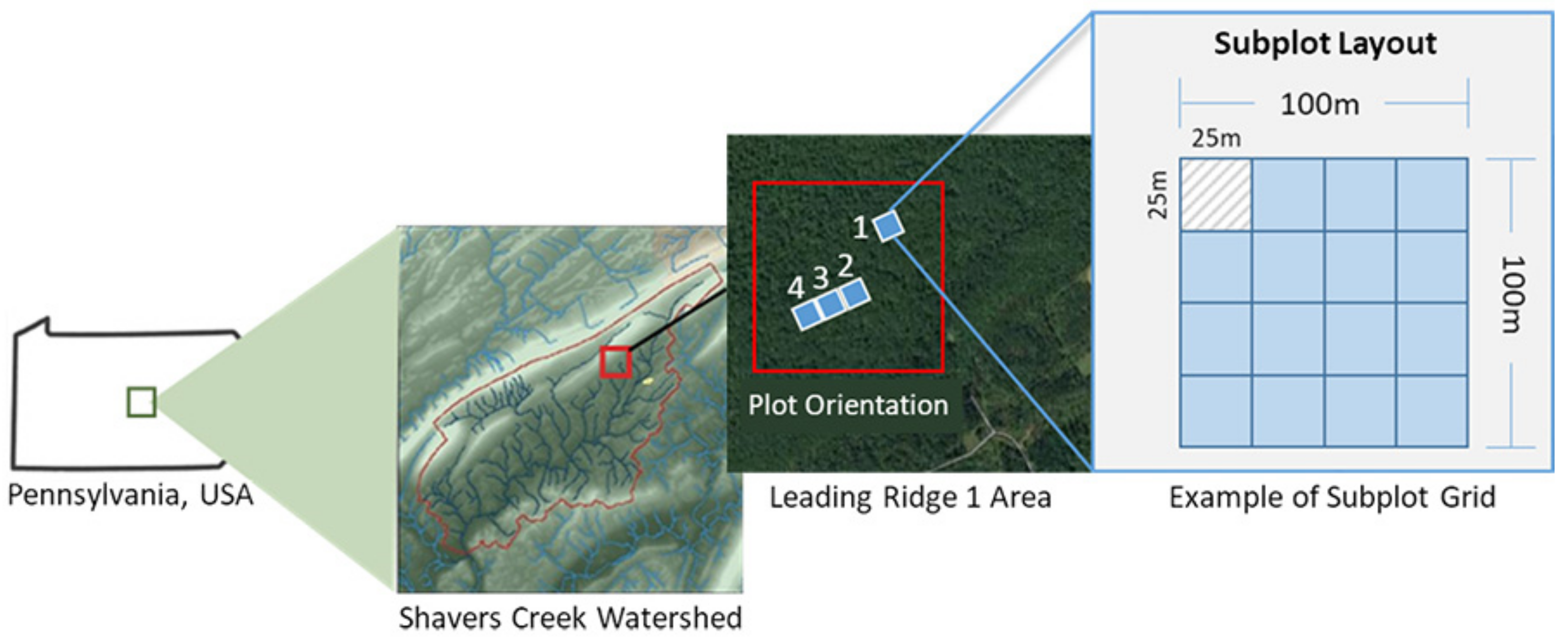
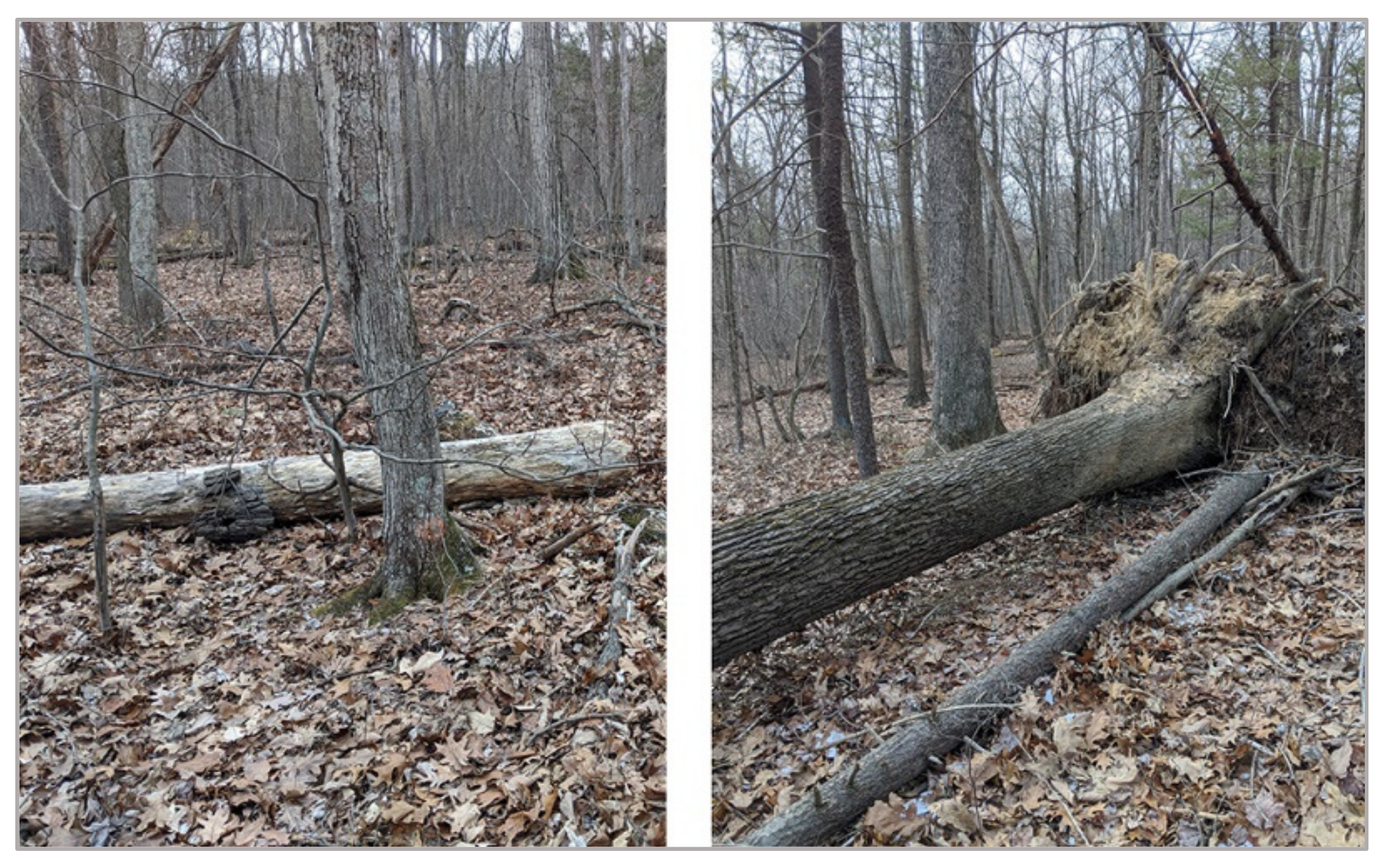
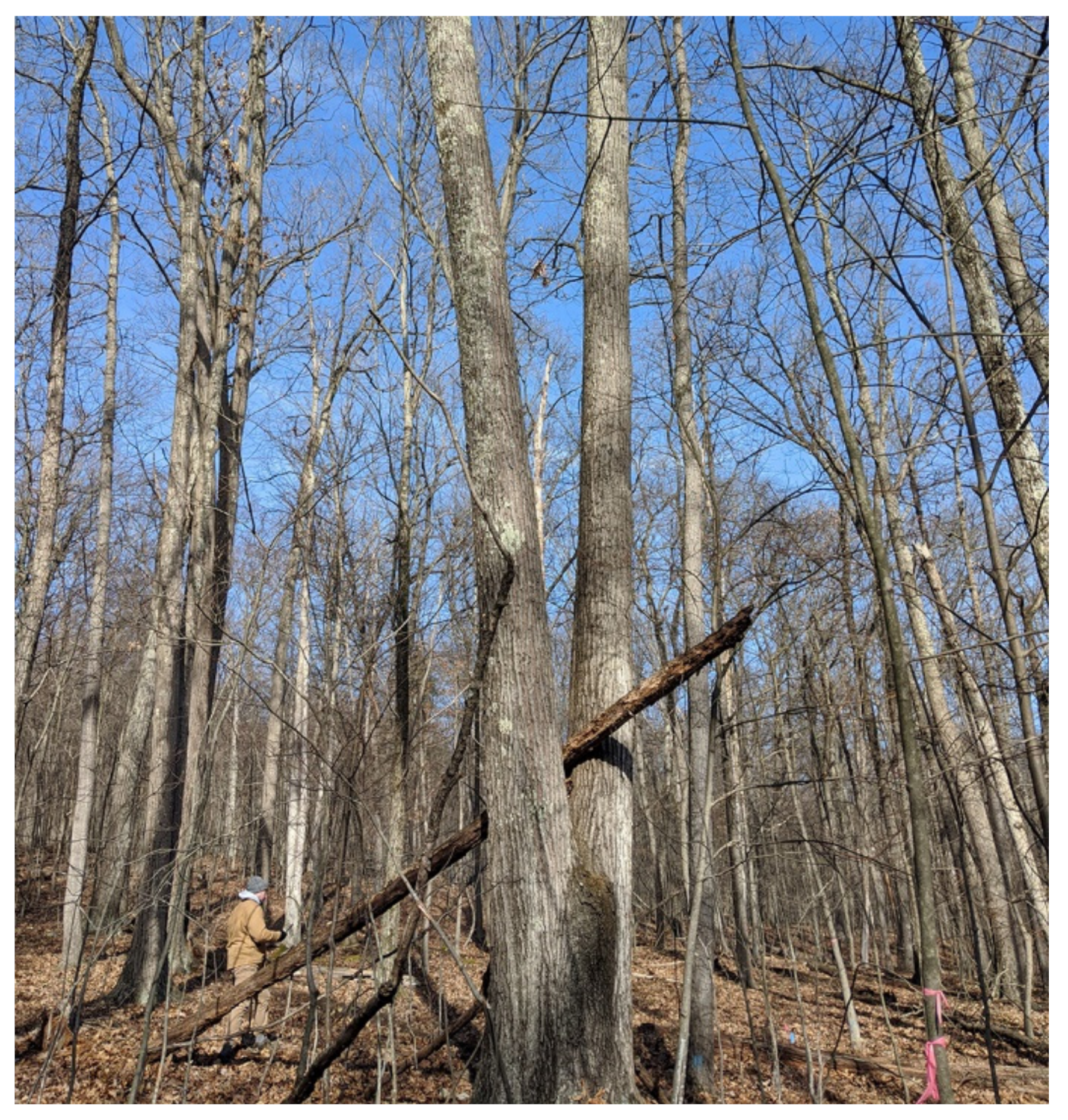
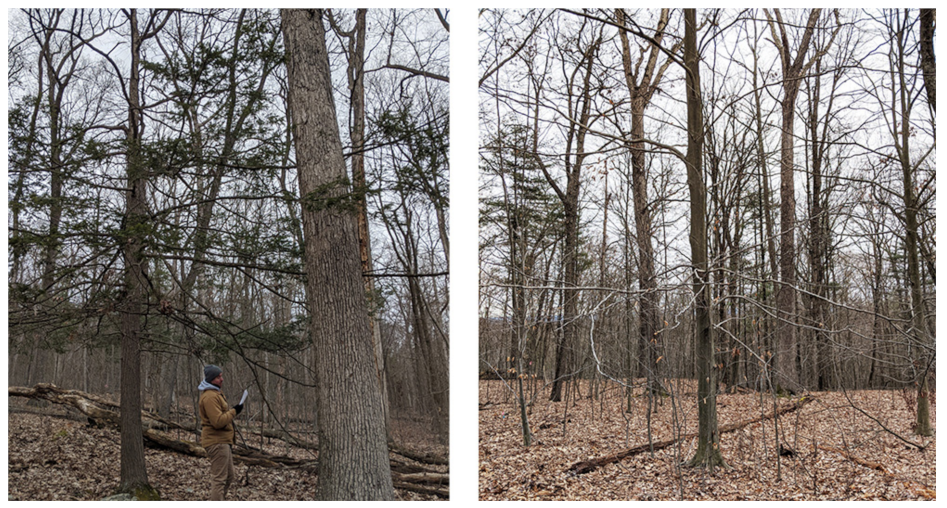
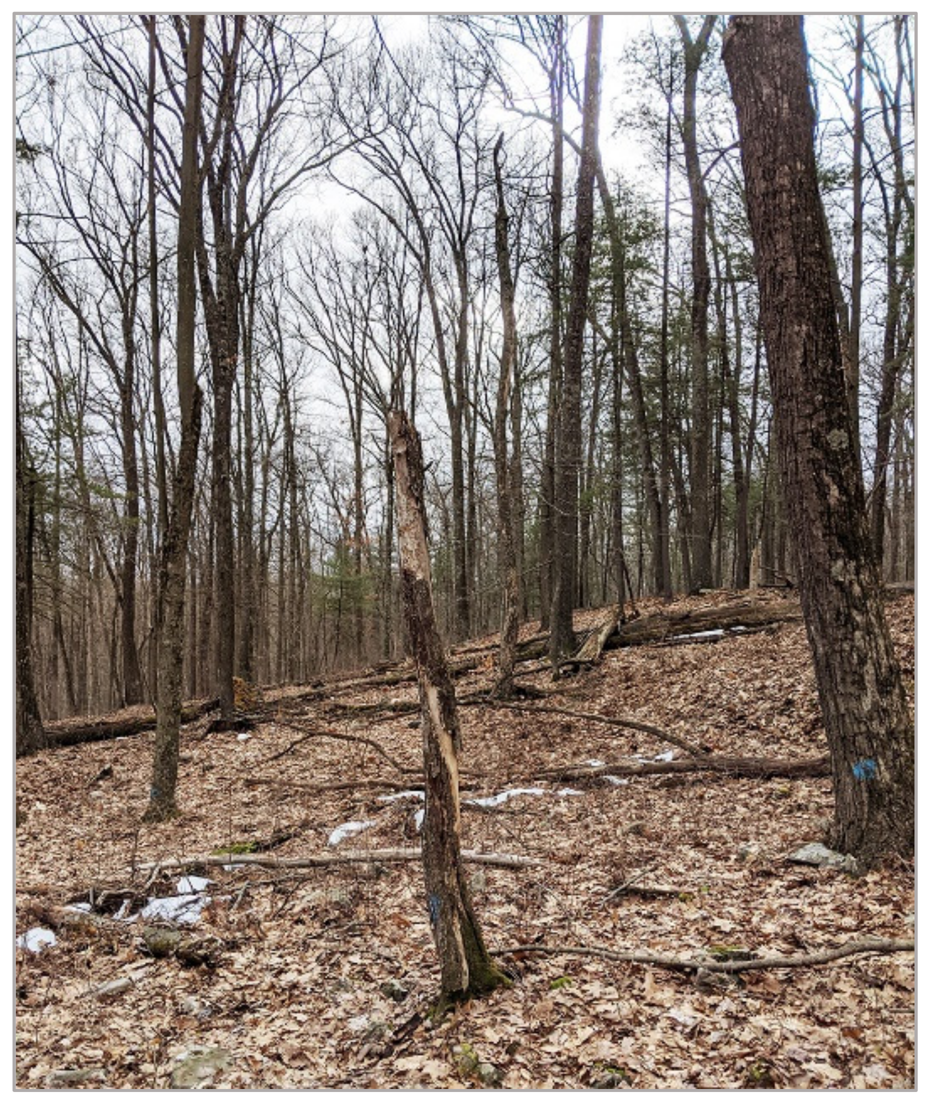
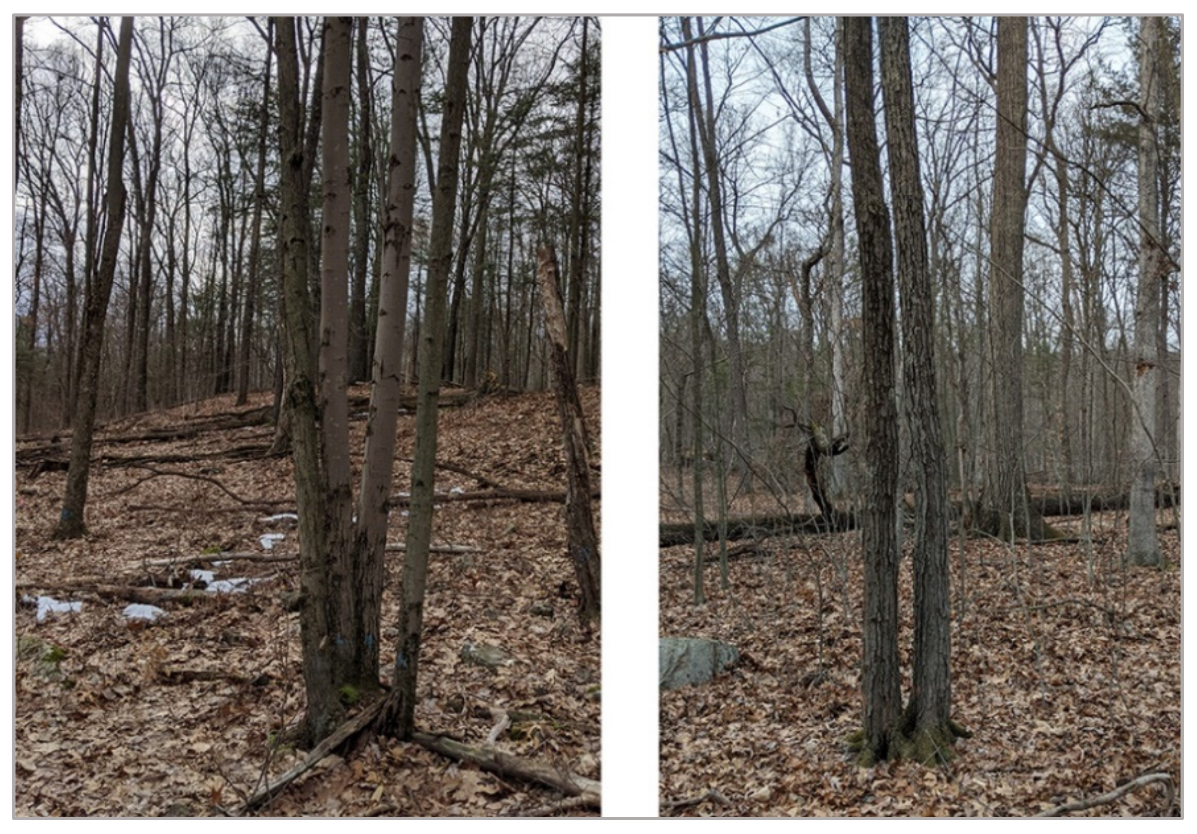
2.1. Study Area

The study area is located in central Pennsylvania, United States, and is comprised of four one-hectare (100 m × 100 m) forest plots. The plots are situated in the Leading Ridge 1 subsection of the Shavers Creek Watershed. Each plot was divided into sixteen 25 m × 25 m subplots, for a total of 64 subplots, with the corner and center points of each marked with durable stakes to enable accurate georeferencing and to support ongoing research efforts. Plot 1 was used to develop and refine or train the method, and plots 2−4 were used as test plots to evaluate the method’s performance. Figure 1 illustrates the relative location of the study area and plots, as well as the subplot configuration.

The study area is in a mature oak-hickory forest stand and has a mean elevation of 331 m, with a range of 315 m to 358 m. The topography varies moderately across the plots, including areas with more ground moisture and narrow waterflows in the lower elevation plots and drier, rockier terrain in the highest elevation plot (Plot 1). These minor variations in terrain are reflected in the tree species composition of the plots, but the predominant species are generally consistent from plot to plot. The most abundant species are hardwood deciduous trees, such as red maple (Acer rubrum), chestnut oak (Quercus montana), white oak (Q. alba), black oak (Q. velutina), blackgum (Nyssa sylvatica), and northern red oak (Q. rubra). Although most of the trees in the study area are hardwood species, approximately 10% are eastern white pine (Pinus strobus) and there is one eastern hemlock (Tsuga canadensis).

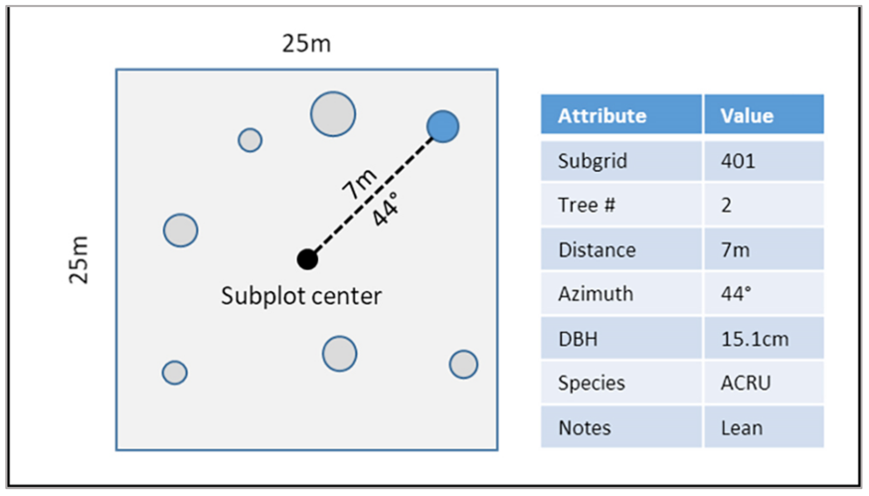
2.2. Reference Tree Data

Ground-based data were collected between summer 2019 and fall 2020 utilizing manual tree survey methods. Measurements were taken using forestry standard tools, including diameter tapes and handheld compasses. Working from the center of each subplot (Figure 2), each tree above 10.1 cm diameter at breast height (DBH) was cataloged and its relative location determined by recording the distance and azimuth reading from the center of the subplot (if obstructed, distance and azimuth measurements were taken from the nearest corner). Stems that forked below DBH were counted as separate trees, following standard forestry practice for the region. During ground data collection, a tree was assumed to be located at the center of the base of the tree. In addition to location, the DBH, species, and any notable characteristics of the trees (e.g., dead trees, forks above DBH, arcs or leans) were noted. Though labor-intensive, these ground data were crucial for both the development of the ITD method and evaluation of its performance. The field-measured tree data include 1467 tree records, including at least 17 species (Figure 3). The mean DBH was 29.01 cm, with a range of 10.16 cm to 100.33 cm and a standard deviation of 16.56 cm. Figure 4 shows the distribution of study area trees by DBH.

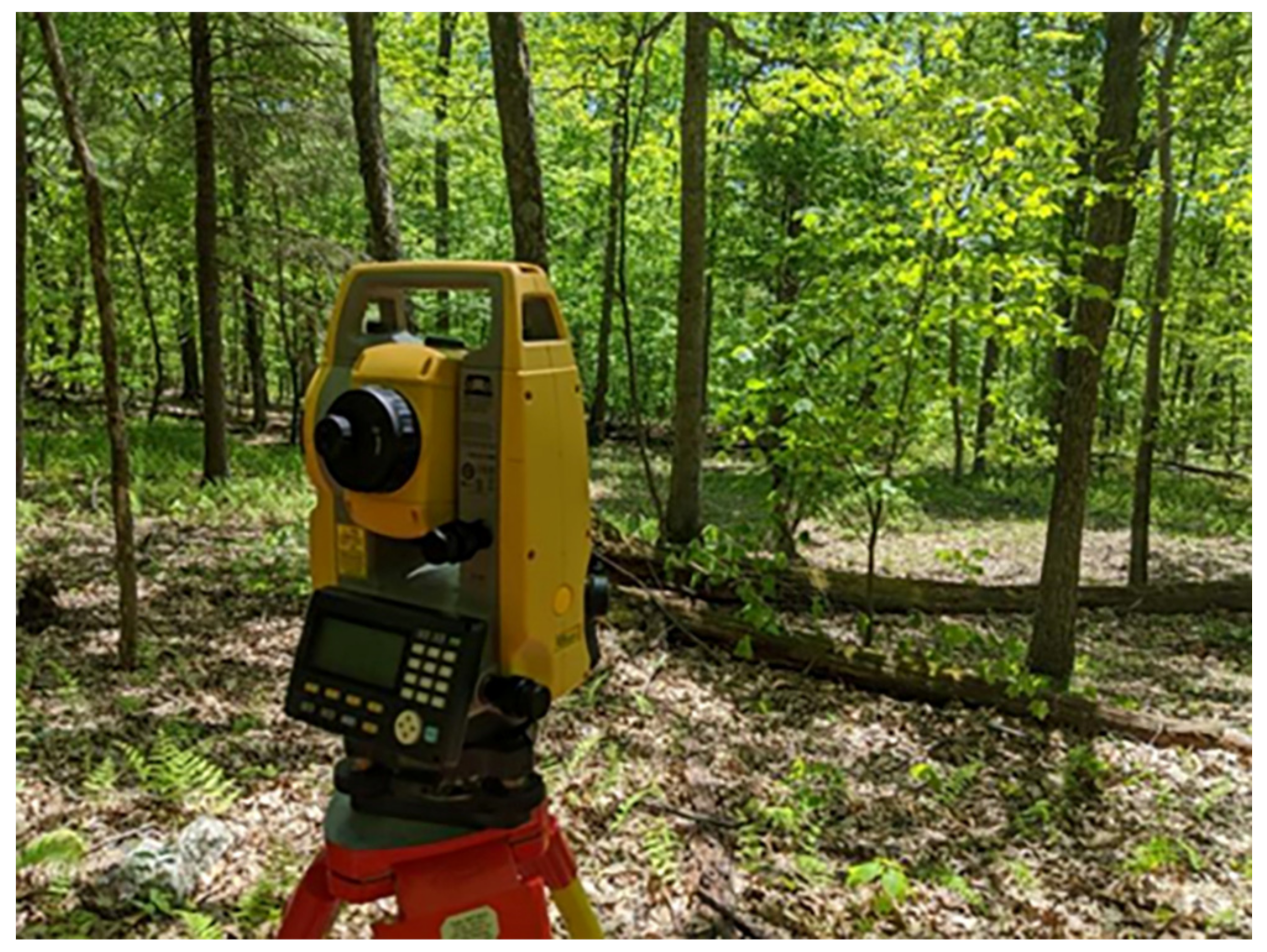
2.2.1. Surveying Ground Plots

Survey-grade instruments were used to accurately georeference the locations of study plot corners and center stakes within a local coordinate system. A TopCon Total Station (ES-105, Topcon Positioning Systems, Inc., Tokyo, Japan) was used to gather relative distances and horizontal and zenith angles between multiple locations within each plot (Figure 5). Standard surveying protocols for back-sighting and number of points measured were followed to ensure accuracy. A constrained least squares regression model was used to generate an accurate grid of the corner and center markers for each of the 64 subplots.

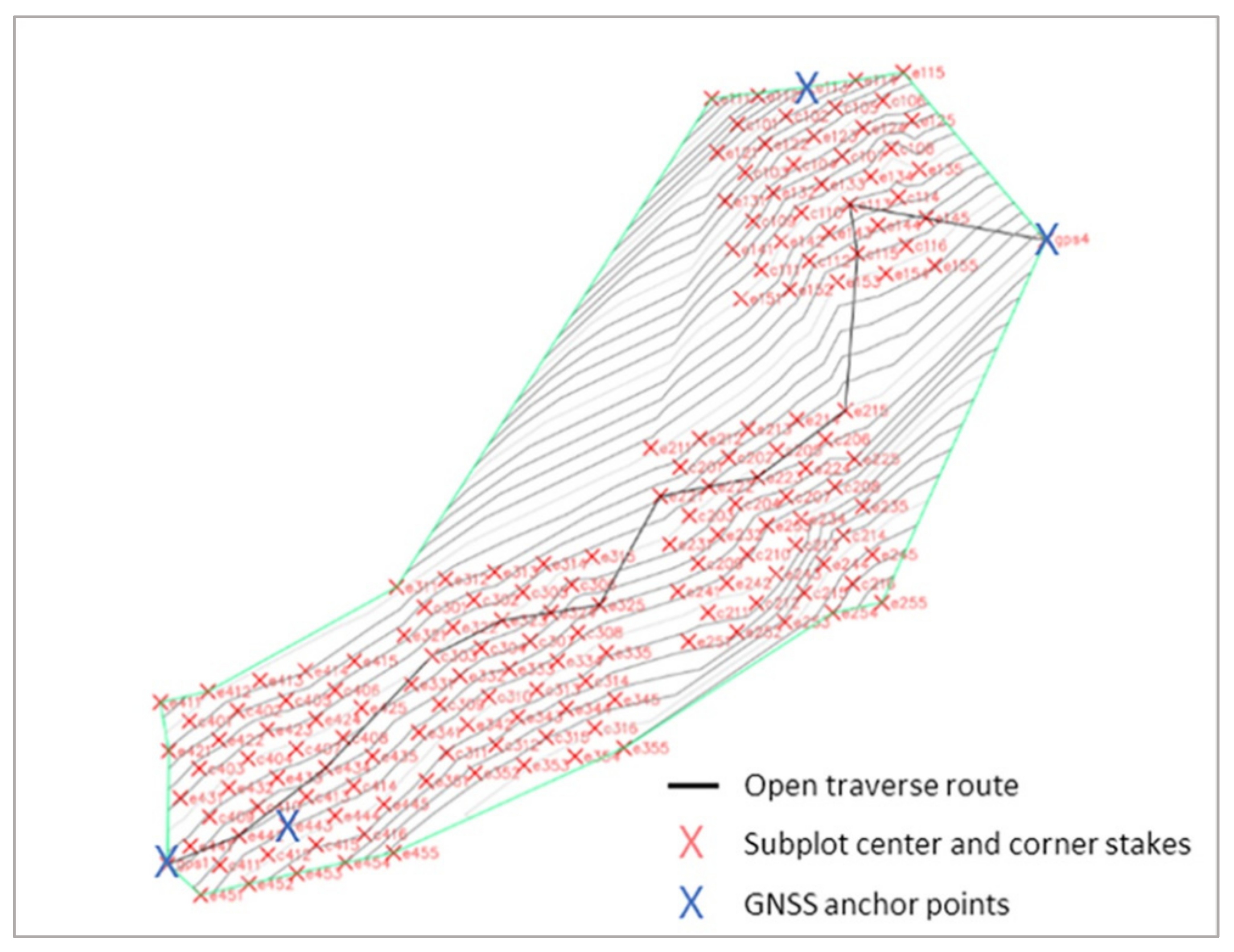
2.2.2. Linking the Local Coordinate System to Geographic Coordinates via GPS

Tree locations were linked to a global coordinate system by placing multi-band GNSS receivers (Emlid, Saint Petersburg City, Russian Federation) at relatively open locations on opposite ends of the grid and gathering satellite signals for several hours to establish high-precision GPS anchor points (Figure 6). An Emlid GPS unit was also placed on a permanent USGS control point approximately 1.6 km from the study area to enable differential correction of the anchor points. An open traverse was performed with the TopCon Total Station to link the anchor points to the grid of center and corner stake locations. This procedure resulted in a mean horizontal accuracy of 11.3 cm for plot corners and centers. To support the ArcGIS Pro [35] portions of the workflow, easting and northing coordinates for each tree were used to create a shapefile for each study plot using the lidR plugin [36] for R software [37].

2.3. Airborne Laser Scanning (ALS) Data

Given the research goal of developing a method to serve as the foundation for operationalizable tools, leaf-off LiDAR was chosen as it aligns with the most widely available datasets in the region. The use of leaf-off LiDAR was also ideal for our voxel-based approach that focused on tree stem detection, as the lack of crown foliage enabled greater penetration of LiDAR pulses and increased the number of pulses that reached tree stems (trunk sections). The LiDAR data used for tree detection were collected in March 2020 by Quantum Spatial, Inc. (QSI) (

Table 1. Technical specification of the ALS data collection.

Attribute	Value
Flight date	22 March 2020
Condition	Leaf-off
Sensor	Riegl VQ1560i
Flying height	950 m
Flight speed	150 kts
Field of view	60°
Scan rate	422 Hz
Pulse rate	2000 kHz
Average point spacing	0.18 m
Average point density	31.2 pts/m2

). A LiDAR sensor (Riegl VQ-1560i, Riegl Laser Measurement Systems GmbH, Horn, Austria) was utilized with a scan angle of ±30° and opposing flight lines with a minimum side-lap of 55%. RMSEz was ≤ 10 cm and the average point density was 31.2 points per m².

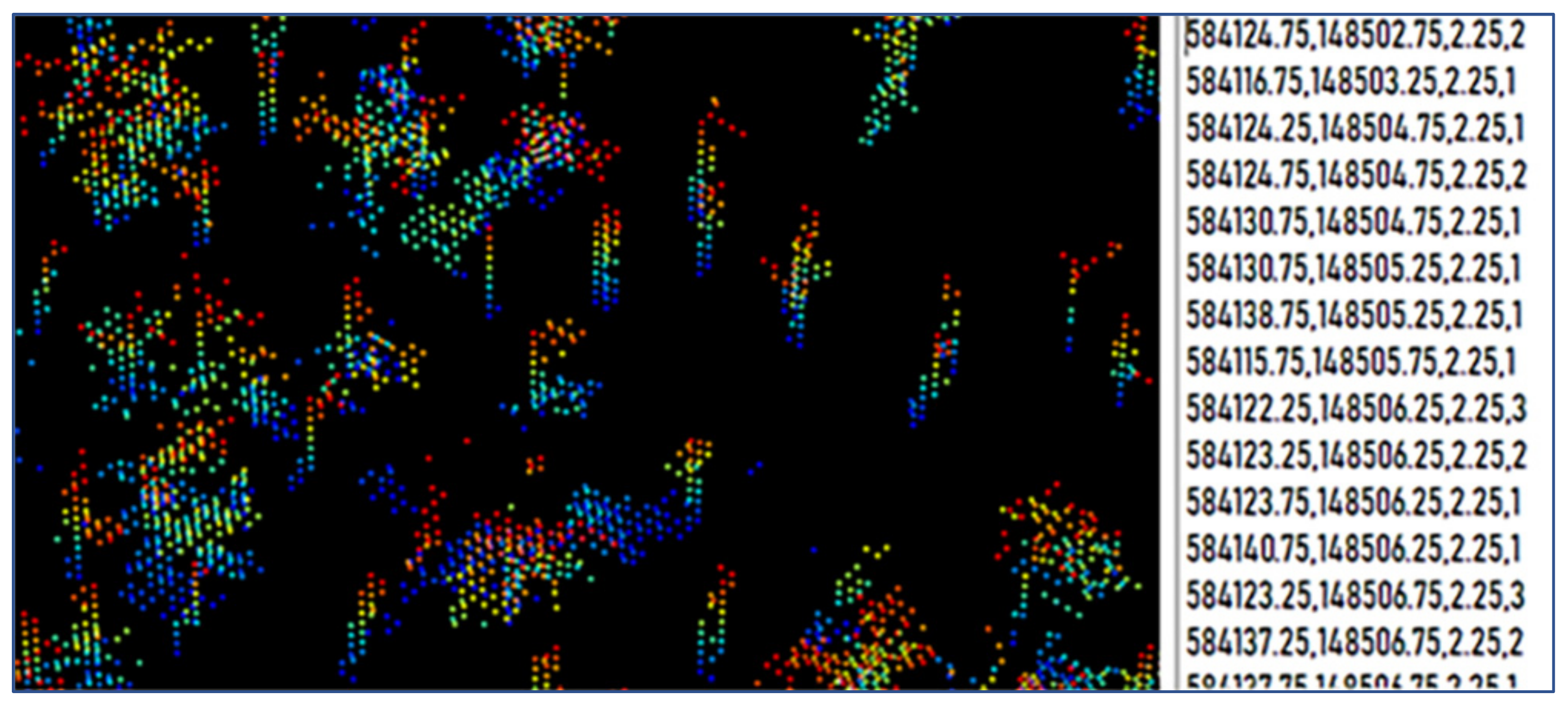
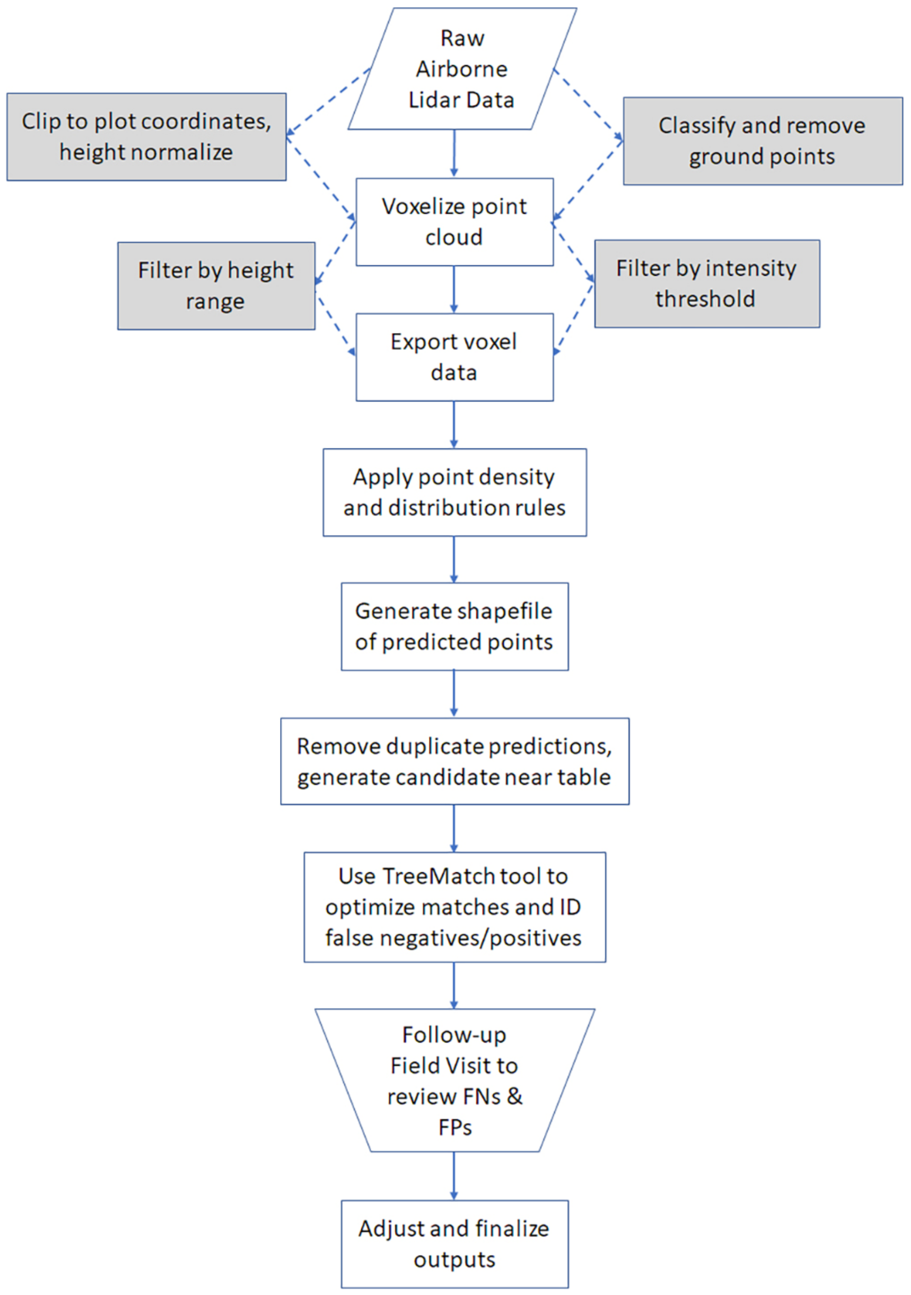
LiDAR Data Preprocessing

The LiDAR point cloud data are stored in tiles measuring 250 m × 250 m that, when abutted edge to edge, create a mosaic of the entire data collection area. Prior to applying the tree detection algorithm, the raw ALS tiles were clipped to the coordinates of the ground plots with a buffer that allowed for variance in ground data collection (e.g., trees slightly outside plot boundaries). These plot-matched point clouds were height-normalized and de-noised, both of which are standard procedures when working with ALS data for tree detection [38]. In addition, ground points were removed to reduce extraneous data and the overall size of the point cloud files. Finally, point clouds were saved in the NAD83(2011)/Pennsylvania South coordinate system, consistent with the other data sources used. All preprocessing steps were performed using LAStools software [39].

2.4. Tree Detection

2.4.1. Background

The choice of a voxel-based approach emerged from initial experiments using established canopy height-based and point-based methods [32,40] with data from the study area and extensive manual visual analysis of LiDAR point clouds. While in some cases tree crowns can be identified in the point clouds, it is often difficult to do so in the mixed-species hardwood forests in our study area. Because the canopy contours are very subtle, canopy height model-based approaches, such as watershed methods, do not reliably determine where one crown ends, and another begins. In addition, what appear to be multiple crown segments are frequently all part of the same tree due to the tree having several large branches. Moreover, the crowns of hardwood trees often are not centered over the tree trunk location due to forking, leaning, and other structural attributes. As a result, even if the crown of an individual tree is successfully segmented, it does not necessarily provide an accurate tree location, making it difficult to link crown segments to ground-based tree records.

Since the existing methods that we tested failed to provide acceptable tree detection performance in our study area, we decided to try to model the pattern recognition humans might use to visually discern trees from the point cloud. In considering how humans visually distinguish trees within the point cloud, tree boles or stems are generally linear, more solid than other features in LiDAR point clouds, and most are readily identifiable visually. For these reasons, a “stem detection” approach was developed to emulate how humans would visually discern individual trees within the point cloud.

While other research [41,42] has focused on region-growing or clustering approaches to build or reconstruct tree stems in the point cloud, these methods can be operationally complex and require considerable computing power—representing significant barriers to scalability. Our proposed method was devised with scalability and simplicity in mind, such that it ultimately can be applied to large datasets and support a broad range of applications where speed and repeatability are key criteria.

The first step in the process is to voxelize the point cloud into 3D bins. These bins serve as an index for the point cloud and enable the application of systematic rules to identify areas with vertical structures, such as tree stems. After testing various voxel sizes, final voxel dimensions of 0.5 m × 0.5 m × 0.5 m were chosen, which provided sufficient granularity while remaining larger than the single tree stems typical of the area. Point clouds were voxelized using LAStools, and the data for non-empty voxels were exported for use in the tree detection algorithm.

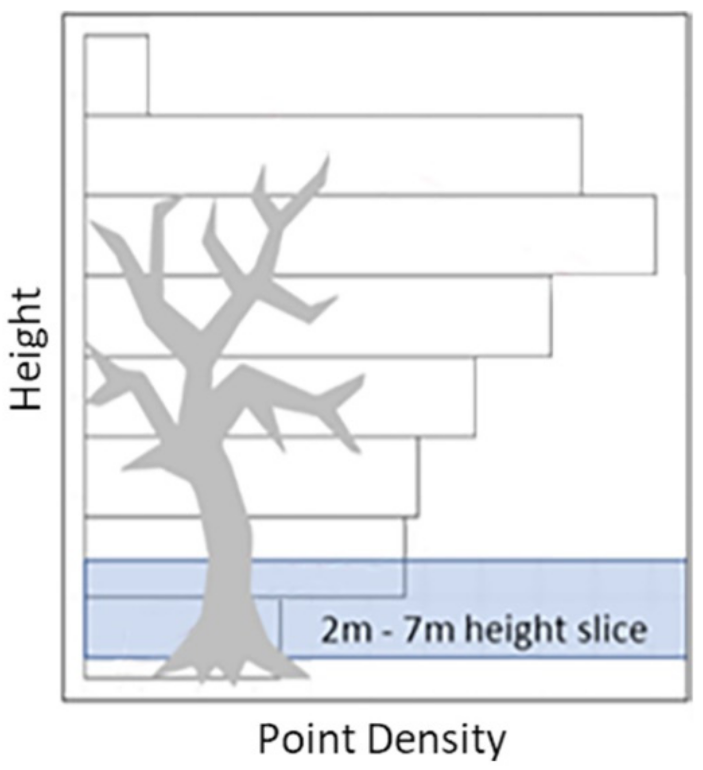
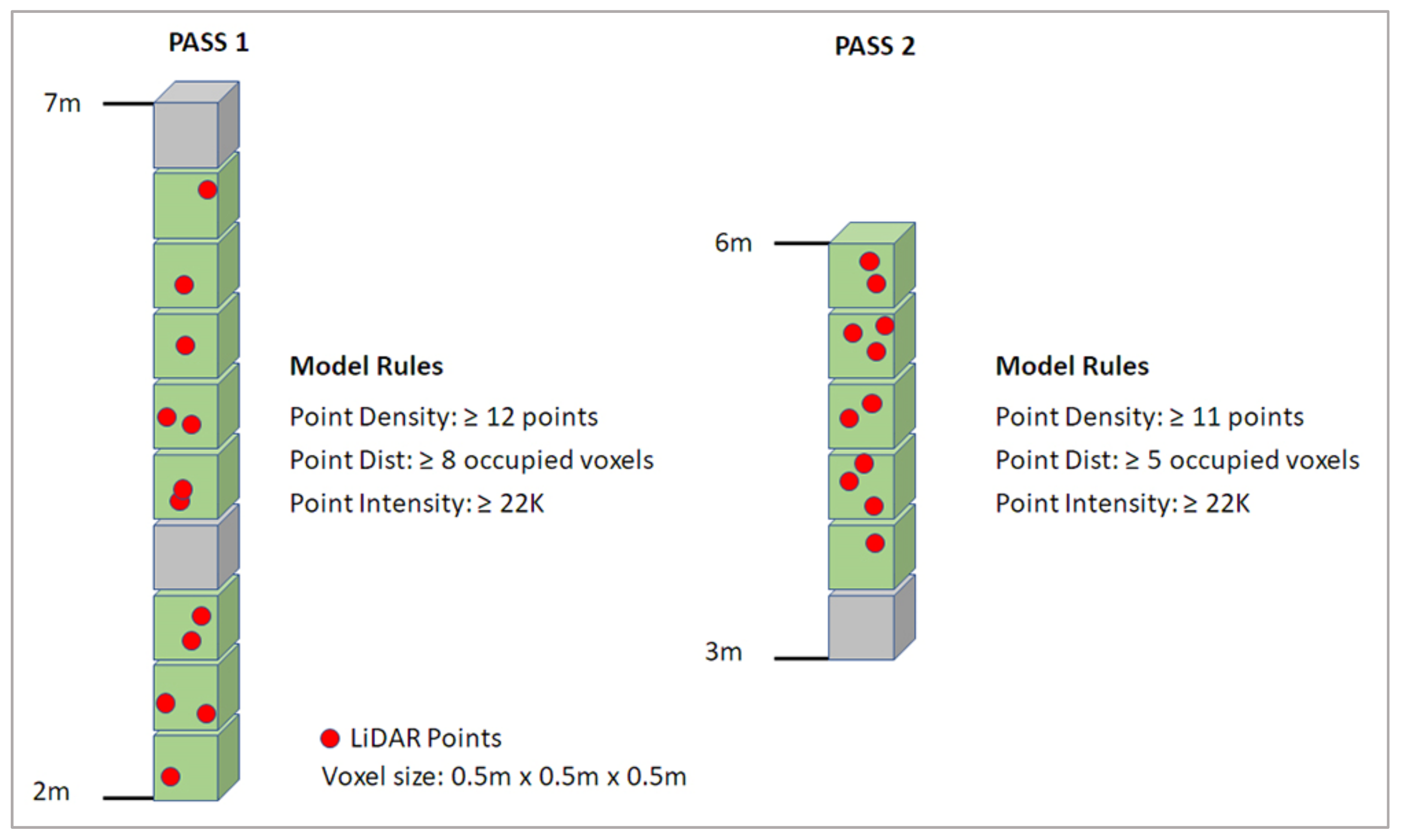
2.4.2. Vertical Segmentation of the Point Cloud

The LiDAR point clouds associated with each one-hectare plot contain over a million points. To efficiently process these clouds and focus on stem detection, we selected a specific vertical range to eliminate points representing the canopy and the dense ground cover often found in northeastern U.S. forests. A histogram of point density (Figure 7) was generated and used (similar to [34,38]), along with field observations, to determine an optimal range of 2 m to 7 m above ground level. This range allows us to efficiently segment and detect tree stems as it excludes low-lying foliage and the major branches of most trees in the plots, providing a clearer perspective of the vertical trunk structures. Segmenting the point cloud in this way also drastically reduced the number of points to be analyzed, resulting in increased efficiency and processing speed, which supports our goal of scalability.

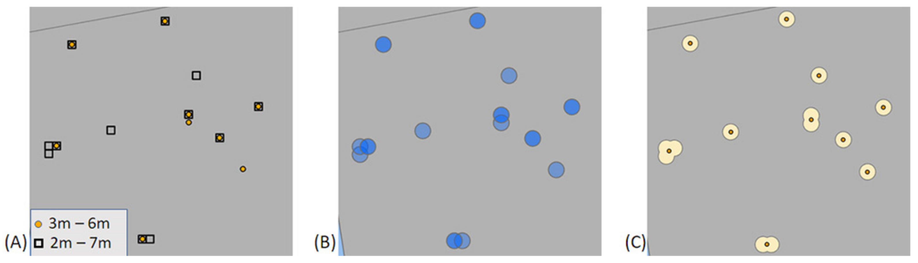
2.4.3. Voxel Column Analysis

The method considers three key factors in identification and assessment of “voxel columns”, or stacks of voxels. Point density, the total number of points in a given vertical voxel column, and point distribution, the number of occupied voxels in a given column, were used as initial indicators of a solid vertical object. To further aid in isolating potential tree stems, LiDAR return intensity was used to filter out smaller, less dense objects, such as branches or foliage. Intensity is a relative value that represents the return strength of each laser pulse and is related to attributes such as surface characteristics and reflectance [43].

Plot 1 was used to develop and refine the rules for the method. The point cloud for Plot 1 was voxelized using LAStools software, and points outside of the 2 m to 7 m vertical slice were excluded. In addition, points with intensity below 22,000 were discarded to filter out smaller branches and non-stem structures [23]. Experimentation indicated that intensity performed well as a filtering variable that helped reduce FPs. The 22,000-intensity threshold was selected based on experimentation with values ranging from 15,000 to 23,000 in intervals of 1000. While lower values yielded more TPs with field measured trees, they also increased the number of FPs disproportionately. Given a key objective was to minimize FPs, the intensity threshold was increased until an optimal balance between minimizing FPs and retaining TPs was achieved.

Data from the voxelized, height-sliced, and intensity-filtered point cloud were converted to text format using LAStools LAS2Text [39] for input to the prediction algorithm. The data output included a 2D coordinate (X,Y), the corresponding vertical height increment, and the count of points for each voxel enabling creation of a voxel column (Figure 8). These data were used to identify candidate voxel columns that might represent a tree.

Rules for point density and point distribution in voxel columns were established iteratively by evaluating tree matching performance for Plot 1. The point density variable gives the total number of points in a column, which contains a total of 10 vertical voxels (5 m height range and 0.5 m voxel size). Rules tuning resulted in a minimum threshold of 12 points for point density. The threshold for the point distribution variable, i.e., the number of occupied voxels (voxels containing a minimum of one point), was set at 8 voxels. To be determined as a valid tree candidate, a voxel column was required to meet the criteria for both point density and point distribution (Figure 9). If both criteria were met, the 2D voxel column location (X,Y coordinates) was identified as containing a predicted tree. Analysis of initial results indicated that the FN rate (missed trees) could be improved by employing a two-pass approach, whereby the voxel data were processed a second time using a narrower vertical range of voxels and different point density and point distribution criteria. A range of 3 m to 6 m was used for the second pass, with values of 11 and 5 for the point density and point distribution, respectively. All voxel columns that met the criteria of either of the two passes were considered tree candidates, and duplicate candidates were identified and eliminated in a later step.

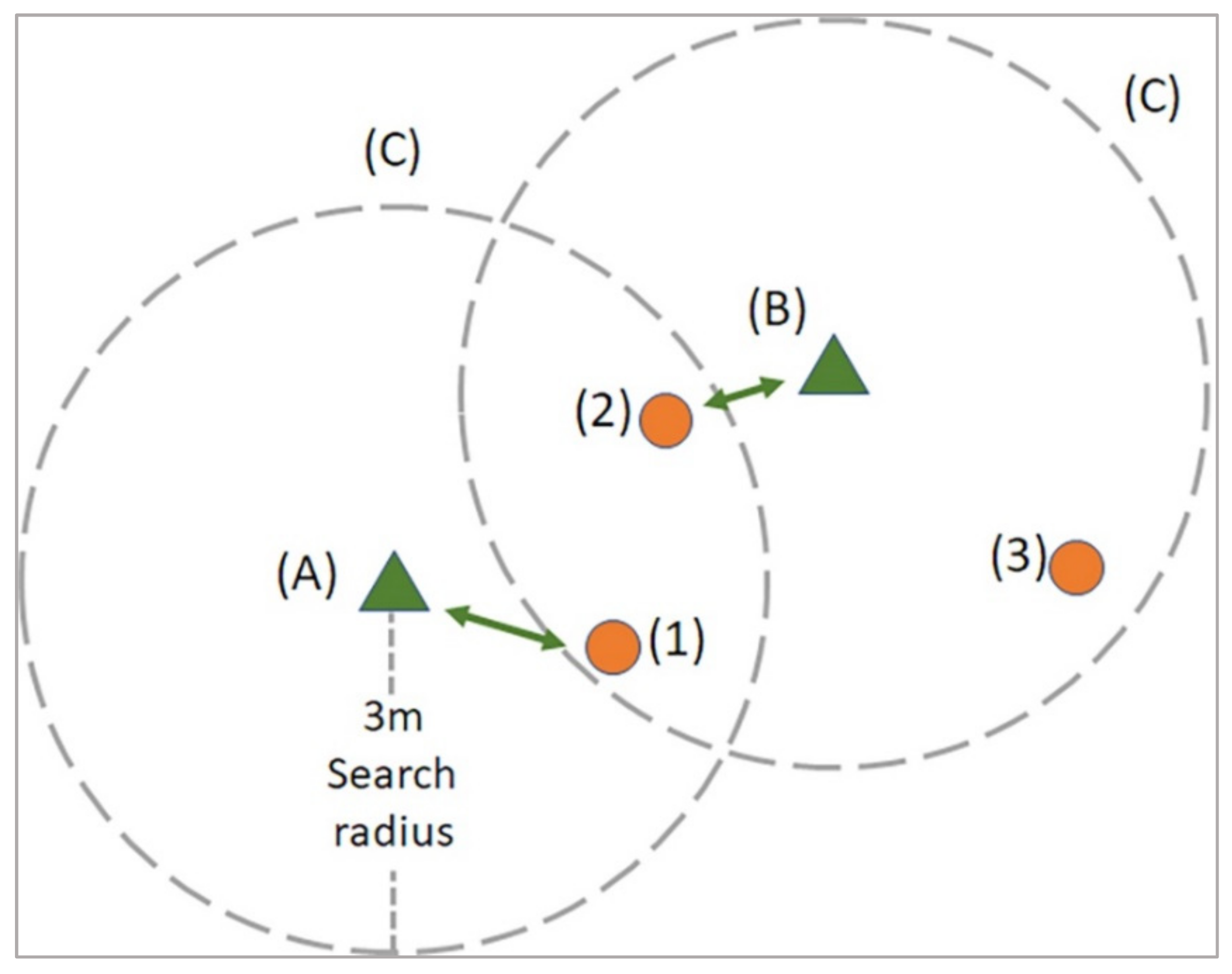
2.4.4. Merging Duplicate Predictions

The output of the two-pass approach is a list of X,Y coordinates for predicted tree locations, which subsequently was converted to a shapefile using R software, enabling visualization and further processing steps in ArcGIS PRO software. As some duplicate predictions were generated, both within each pass and between the two passes, a process to merge predicted tree locations was devised. This process involved creating a 0.5 m buffer polygon around each predicted point, dissolving overlapping buffers, then finding the center of the resulting polygon and assigning those coordinates to the predicted tree location. Figure 10 illustrates the major steps of this process, which eliminated a significant number of duplicates that were within 1 m of each other, with a minimum negative impact on the overall detection rate that might result from merging two nearby predictions that were, in fact, two separate trees.

2.4.5. Tree-Matching and Evaluation Process

In order to evaluate how well a tree-identification algorithm performs, it is necessary to determine the number of correctly identified trees (TPs), the number of missed trees (FNs), and the number of predicted trees that do not correspond to actual trees on the ground (FPs). This requires a matching process where predicted trees are matched with reference trees—i.e., actual trees on the ground. It is not necessarily obvious how to match predicted trees to reference trees (known trees based on ground observations), and no consistent approach for accomplishing this has been discussed in the literature. Given our secondary objective of generating an accurate tree map, positional accuracy was a core factor in evaluating performance. A predicted tree was only considered a match to a reference tree if its position could be confidently associated to that of the reference tree, and both the evaluation approach and the matching algorithm itself were developed with this in mind.

To manually assess performance based on more than 1000 reference trees would be tedious and time-consuming to accomplish. More importantly, manual matching leaves room for subjectivity, as two people may match a given predicted tree to different reference trees. An automated, repeatable method of matching predicted trees to reference trees would avoid issues with manual matching. This method should satisfy three rules, or constraints: (1) a reference tree can be matched to at most one predicted tree, (2) a predicted tree can be matched to at most one reference tree, and (3) the distance between a predicted tree and a matching reference tree must be less than some specified maximum. The objective of our procedure was to minimize the total distance between matched pairs of trees.

An application named TreeMatch was developed that utilizes linear integer programming to optimize the predicted-to-reference tree matches following these rules. As input into the TreeMatch application, ArcGIS PRO was used to generate a “near table” based on the reference and predicted tree locations. The “near table” is a CSV file containing lists of all predicted trees within a 3 m radius of each reference tree. The TreeMatch application, built using Microsoft Visual Basic, uses the CSV data to create a linear integer programming model (Equations (1)–(5)) as a text file. The Gurobi solver [44] was then used to solve the linear integer programming model to optimize the matching of reference trees to predicted trees using a minimum distance method.

$$\mathrm{Minimize} {\displaystyle \sum }_{jϵJ}{\displaystyle \sum }_{kϵ{\mathsf{\Phi }}_j}{d}_{j,k}{X}_{j,k}$$

(1)

Subject to:

$${\displaystyle \sum }_{kϵ{\mathsf{\Phi }}_j}{X}_{j,k}\le 1 \forall jϵJ$$

(2)

$${\displaystyle \sum }_{jϵ{\mathsf{\Psi }}_k}{X}_{j,k}\le 1 \forall kϵK$$

(3)

$${\displaystyle \sum }_{jϵJ}{\displaystyle \sum }_{kϵ{\mathsf{\Phi }}_j}{X}_{j,k}\ge min\left\{\left|J \right|, \left|K \right|\right\}-i$$

(4)

$$X_{j,k}ϵ\left\{0,1\right\} \forall jϵJ, kϵ{\mathsf{\Phi }}_j$$

(5)

where SETS: J = the set of known (reference) trees, K = the set of predicted trees that can potentially be matched with at least one known tree j ϵ J (predicted trees that have no potential match in J are automatically classified as false positives and removed from the problem definition); Φ_j = the set of predicted trees, k ϵ K, that are candidates for a match with known tree j ϵ J (note that there is one of these sets for each known tree j ϵ J and all Φ_js are non-empty by design); Ψ_k = the set of known trees, j ϵ J, that are candidates for a match with predicted tree k ϵ K. Again, there is one such set for each predicted tree k ϵ K and all Ψ_ks are non-empty by design. PARAMETERS: d_j,k = the distance from known tree j to predicted tree k; i = feasibility parameter, which is initially set to zero and is incremented by one until a feasible solution is obtained. VARIABLES: X_j,k = 1 if known tree j is matched with predicted tree k and 0 otherwise.

The model (Equations (1)–(5)) maximizes the number of feasible matches while minimizing the total distance between pairs of matched trees and satisfying the constraints that (1) a predicted tree can be matched to at most one reference tree, (2) a reference tree can be matched to at most one predicted tree, and (3) the number of matches must be greater than or equal to some minimum. The minimum of (1) the number of reference trees, and (2) the number of predicted trees is an upper bound on the maximum number of feasible matches, but the actual number of feasible matches can be less than this upper bound if, for example, two predicted trees can only be matched to a single reference tree. The parameter i is initially set to zero and incremented by one until a feasible solution is achieved. The output of this model is a set of matched pairs of predicted and measured trees. As noted, a 3-m search radius was used to generate the near-matches of predicted trees for each reference tree (Figure 11).

2.4.6. TreeMatch Data Postprocessing

Several postprocessing steps were performed on the resulting TreeMatch output data prior to analysis. Trees located outside of a 1.5 m buffer around the plots were removed from the results. Measured trees that were cataloged individually but noted as being part of a multi-stem tree (2 or more stems from same trunk that split below DBH) were reviewed to correct FNs (Figure 12). In some instances, multiple stems were detected as one tree within a 0.5 m² voxel, creating a number of FNs. Adjusting the data for such instances resulted in 26 FNs being reclassified as TPs across the three test plots.

Follow-up field visits, which are rarely reported in the literature, were made to visually investigate all FPs (commissions) in the three test plots as well as FN (omissions) for notable reference trees (e.g., larger DBH trees, snags). This effort provided extremely valuable context for the FP and FN results and enabled the identification of some trees that had fallen (Figure 13) between the ground-based observations and the LiDAR data collection (and were therefore not actually FNs). The visits also identified several trees for which location data were transposed by the ground crew and a number of trees that were not cataloged (missed) during the tree survey work. These trees were location-corrected and added to the ground truth tree dataset, as appropriate, and the results adjusted to reflect these changes.

Figure 14 summarizes the steps in the individual tree identification procedure from the initial raw LiDAR data set to the field verification step.

3. Results

3.1. Overall Tree Detection Performance

Of the 1125 total trees across the three test plots, our method detected 762, representing an overall detection rate of 67.73%. Detection rates for test plots 2, 3 and 4 were relatively consistent at 65.88%, 67.70%, and 69.82%, respectively. Detection rates across the 48 subplots had a standard deviation of 9.33% and standard error of 1.35% (

Table 2. Summary statistics for detection rate across the 48 study subplots.

Attribute	Value
Test Subplots	48
Total Trees	1125
Trees Detected (TPs)	762
False Negatives (FN)	363
False Positives (FPs)	38
False Positive Rate	4.75%
Overall Detection Rate (DR)	67.73%
Minimum DR (across 48 subplots)	47.62%
Maximum DR (across 48 subplots)	85.00%
Mean DR (across 48 subplots)	68.00%
Median DR (across 48 subplots)	68.21%
Standard Deviation for DR (across 48 subplots)	9.33%

). Of 800 predicted trees, 38 were determined to be FPs, for an overall FP rate of 4.75%. Within individual 25 × 25 m subplots, detection rates varied from 47.6% to 85%, indicating that the tree detection algorithm performs consistently well even at this scale. These results are discussed in more detail in subsequent sections.

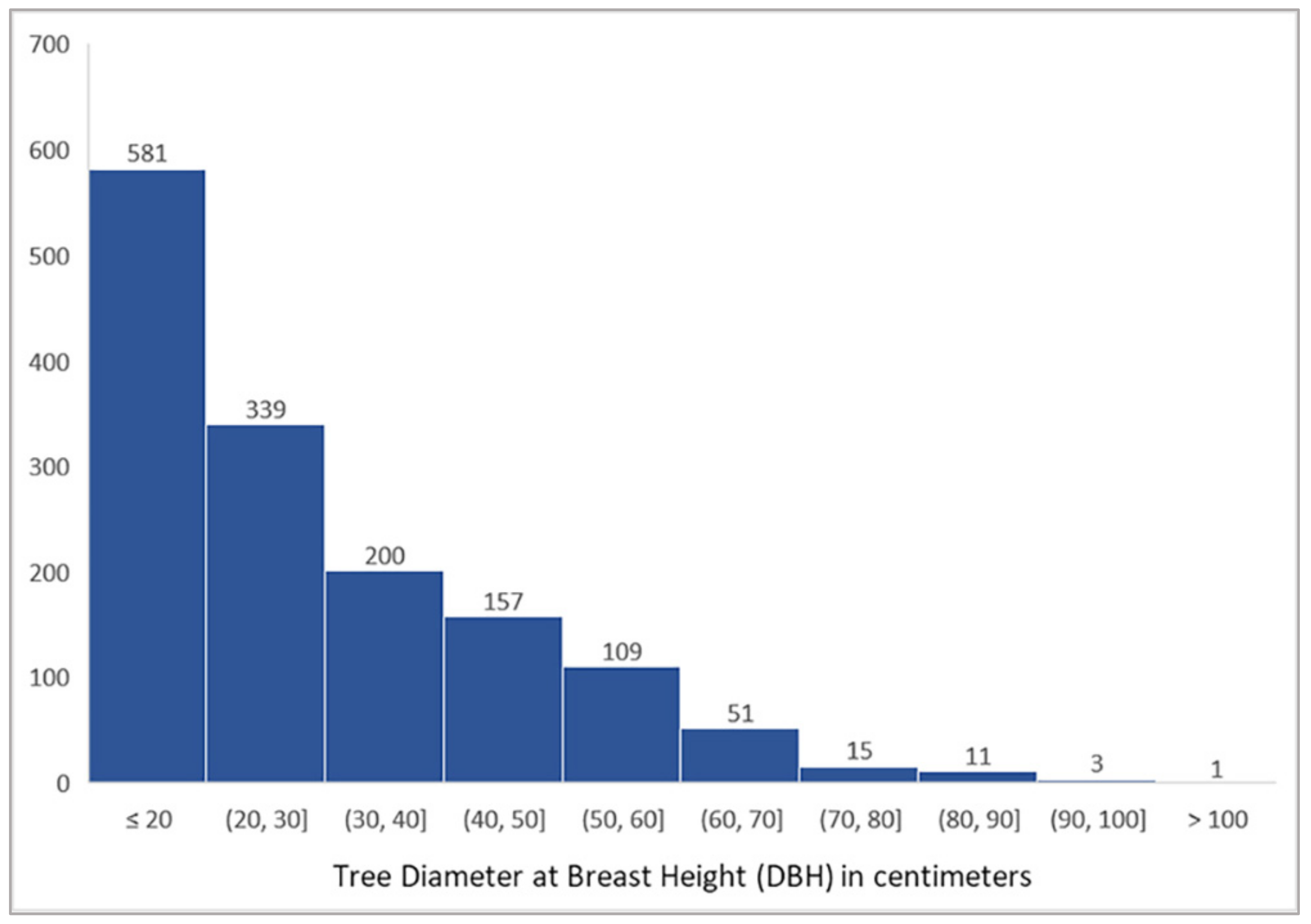
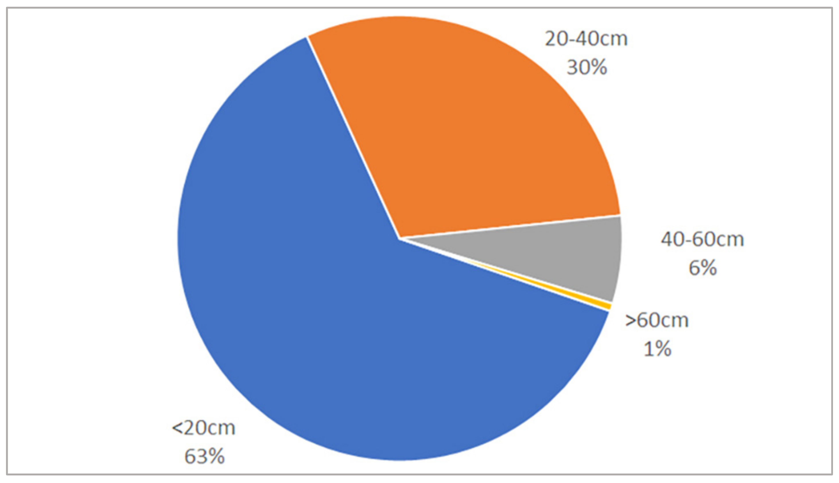
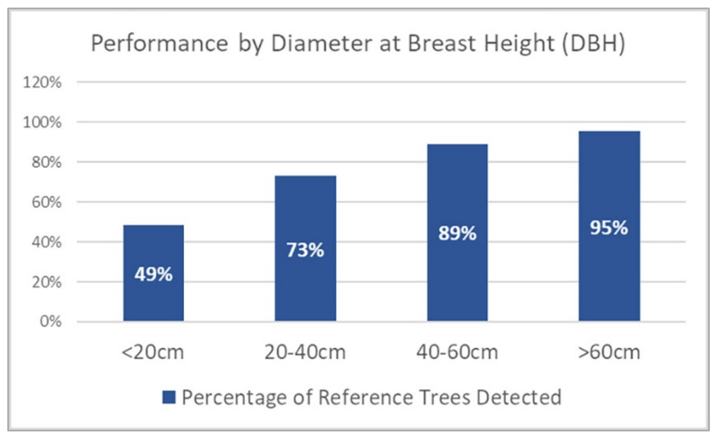
3.2. Tree Detection Performance by DBH Range

The algorithm’s tree detection performance was strongly linked to DBH and improved notably as tree diameter increased (Figure 15). While trees with DBH under 20 cm were detected at a rate of 49%, the rate was 86.5% for trees above 28 cm DBH (the minimum DBH for sawtimber). For the largest trees in the study plots, those with DBH greater than 60 cm, only 3 of 64 trees were not detected.

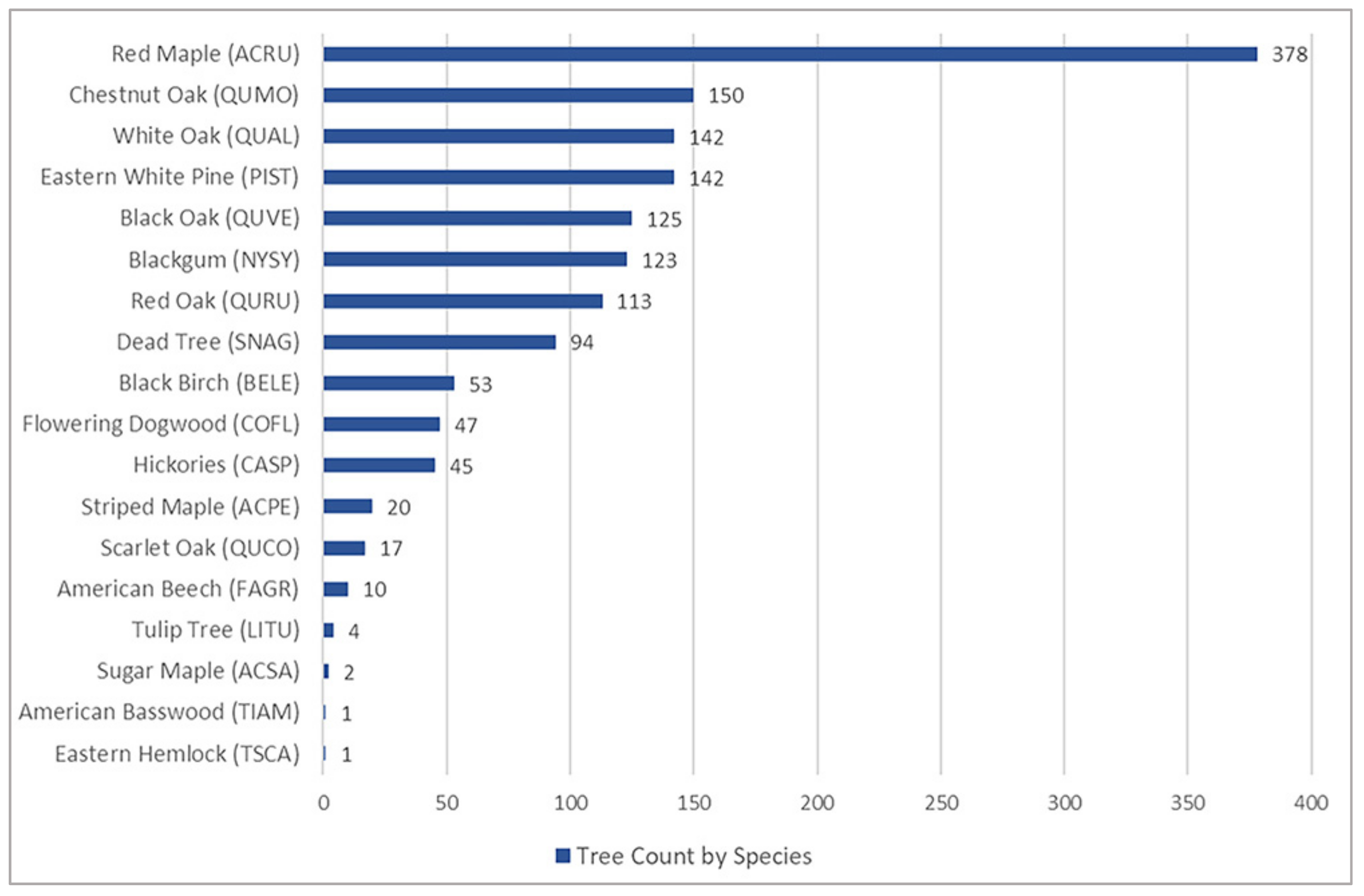
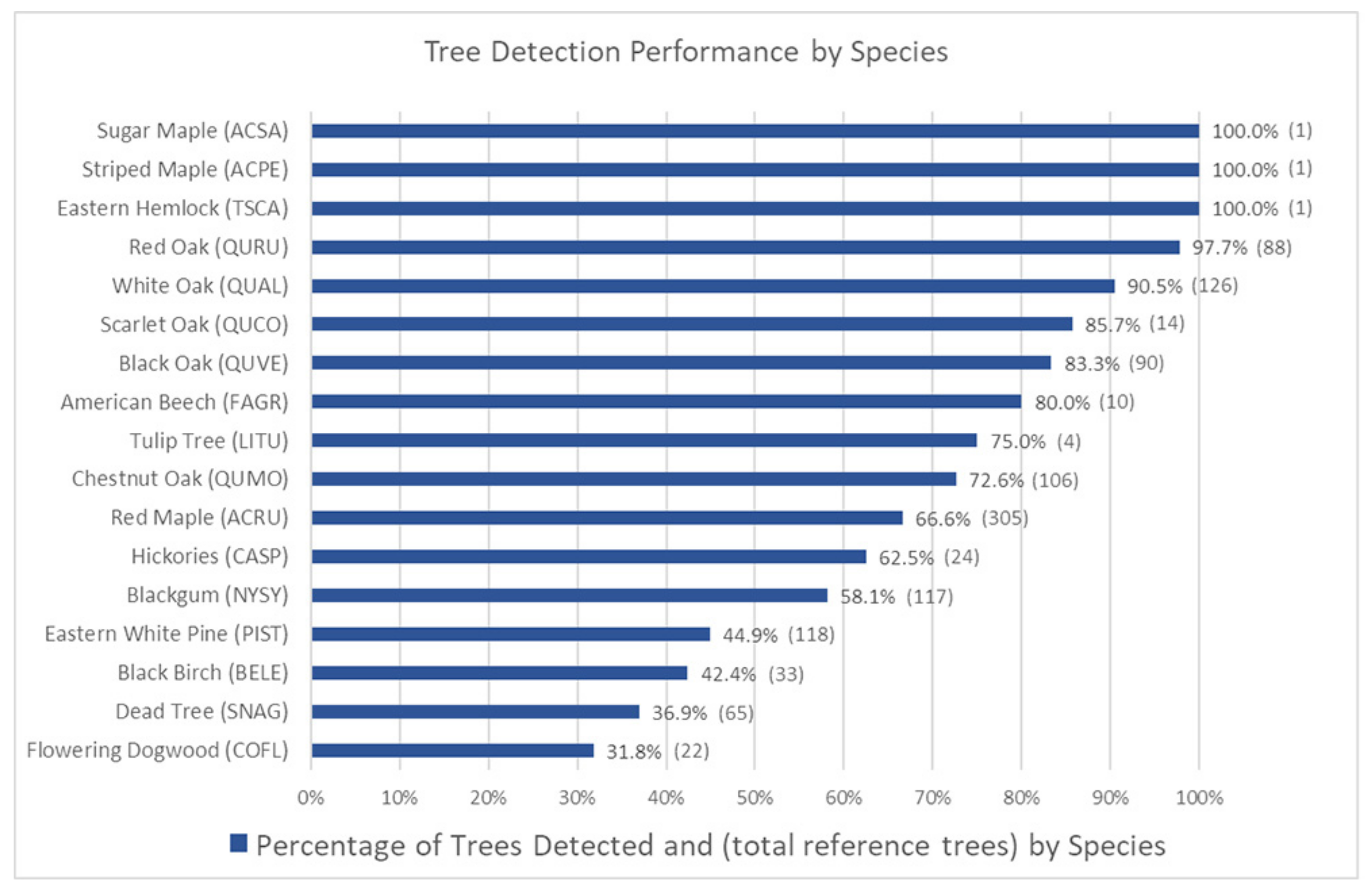
3.3. Tree Detection Performance by Species

With the possible exceptions of eastern white pine, which has a diffuse and distinct branching structure relative to the other species in the study plots, and snags (dead trees), which are often short or leaning, most species-related variations were strongly linked to DBH. The seven least-detected tree species all had mean DBH values less than 23 cm, while the larger oak species were detected at much higher rates. Figure 16 provides a breakdown of the performance by species.

3.4. False Positives

False positives (FPs) were defined as predicted tree locations that were not matched to a reference tree. Initially, 59 FPs were identified across the three test plots. Follow-up field visits enabled review and analysis of each FP instance. Twenty of these FPs were trees that either were not recorded in the ground-based tree survey or had their locations entered incorrectly, and one FP outside of the plot boundary was removed from analysis. This resulted in a corrected FP count of 38.

Of the remaining 38 FPs, based on their location, 31 appeared to be detecting small trees that were under the 10.1 cm DBH threshold to be recorded in the ground-based tree survey. Three FPs were confirmed to be the 2nd stem of large, forked trees that were recorded as a single tree in the ground survey per the protocol (Figure 17). The remaining four false positives included two instances of branching that was dense enough to be interpreted as a tree (Figure 18), and two instances where the predicted location simply contained no tree within the allowed maximum radius for matching.

Thus, although we report 38 FPs, after field verification, only four of those were “true” FPs that clearly did not correspond to a real tree stem on the ground (two were detections of branches). Thus, in effect, we reduced the number of FPs to practically zero, and further attempts to reduce FPs would likely be counterproductive.

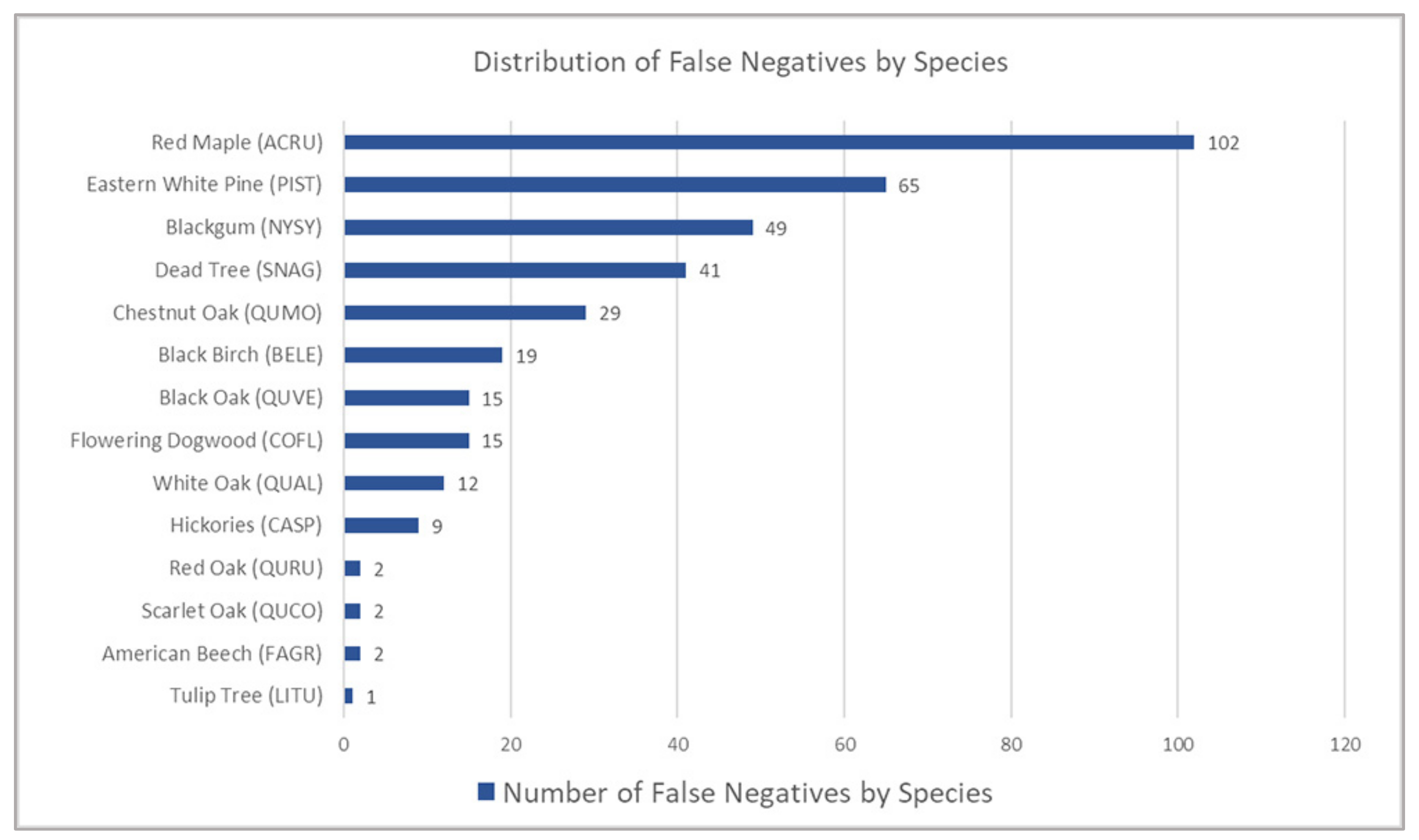
3.5. False Negatives

False negatives (FNs) were defined as reference trees that were not matched to a predicted tree. As noted previously, most FNs (63%) occurred with trees <20 cm DBH. Figure 19 provides a more detailed breakout of all FNs. A distribution of FNs by species is provided in Figure 20.

For FNs, or missed trees, the field follow-up visits again were quite valuable. While each FN was not reviewed, a significant number of particularly large DBH trees and trees noted as snags, which might be difficult to detect, were reviewed. This effort identified several downed trees and short snags (Figure 21) that were outside of the detectable range based on the algorithm rules. Several patterns among FNs were observed, including leaning or curved boles, suggesting that these trees were not detected due to their tendency to span several voxel columns in the detection height ranges used. Voxel sizes larger than 0.5 m were tested in the development phase, but resulted in overall poorer results, so a different approach must be taken to address leaning trees. The algorithm detected less than half of the eastern white pines in the study area, likely due to the low, diffuse branching structure of this species, which tends to disperse the LiDAR returns. In addition, proximity to eastern white pine trees also contributed to FNs, likely due to the dispersal of the LiDAR returns by the pines’ branches (Figure 22). This could be considered a “neighborhood effect” [5] and warrants further exploration.

3.6. Spatial Accuracy of Detected Trees

Spatial accuracy was a requirement in validating predicted trees as detected by the algorithm and was an integral part of both the development and evaluation of the method. Though we used a 3 m search radius to generate candidate predicted trees around ground-measured reference trees for the tree match methodology, over 80% of matched predicted trees were within less than 1 m of their associated reference tree, with a mean distance of 0.59 m (

Table 3. Summary statistics for measured tree to predicted tree distance.

Attribute	Value
Total Matches	742 *
Minimum	0.020 m
Maximum	2.999 m
Mean	0.590 m
Median	0.460 m
Standard Deviation	0.504 m

* The 20 trees identified as missed or mislocated in the ground survey were assigned the coordinates of the predicted location resulting in a distance of zero, thus these data points were omitted from this analysis.

). The high level of spatial accuracy of the matches was evident in field follow-up visits where locating FPs was relatively straightforward due to the precision of location data for both reference and predicted trees. Furthermore, there were multiple instances where the positional accuracy of the trees detected from ALS data was greater than that of the ground survey, which aided in identifying location transcription errors and unrecorded trees.

4. Discussion

4.1. Context and Interpretation of Results

The overall tree detection performance of the proposed method was robust at 67.73% of all reference trees (trees ≥10.1 cm) and 86.5% for trees ≥28 cm with a very low observed commission (false positive) rate of 4.75%. These results, which include all diameter classes, compare favorably with other methods where detection rates for intermediate and suppressed trees were substantially lower [10,20,25]. That said, given the lack of standardized evaluation criteria and the overwhelming focus on conifer-dominated forests in the literature, it is difficult to directly compare our method’s performance with previous studies. Prior evaluation methods ranged from manual validation of detected trees [29] to ratio-based approaches (number of reference trees compared to predicted trees for a plot) that often ignore positional accuracy [20,23,40]. In some cases, an attempt was made to match detected trees to reference trees, yet no average or maximum predicted-to-reference tree distance was provided [13,14,22]. As such, it is crucial to view this study’s results in the context of the new quantitative evaluation methods employed and the stringent criteria established for declaring a tree as “detected,” which require both a one-to-one match between a predicted tree and a reference tree and a spatial accuracy component. Further, minimizing false detections or commission errors was a key priority in tuning the method. This resulted in highly reliable tree detections and accurate predicted stem locations; there is essentially no chance that a FP was mistaken for a TP. The proposed algorithm can be tuned to provide a higher overall detection rate, but the tradeoff is an increase in commission errors (FPs), which we believe diminishes the reliability and usefulness of the output. Since the ultimate goal is an operational tool, the decision was made to prioritize the minimization of FPs in order to establish a reliable baseline detection rate. This perspective differs from the stance taken in a benchmark study of five recently developed ITD methods [25] wherein a relatively high commission error (e.g., >30%) was considered an acceptable cost of obtaining higher tree detection rates. The capability of the proposed method to achieve an overall detection rate of nearly 68% across all reference trees of all sizes (dominant, intermediate and suppressed), with a raw commission rate of less than 5%, is a clear indicator of its contribution to the ITD space. Furthermore, as discussed above, most of the FPs were likely actual tree detections. Many were simply smaller than the threshold to be measured in the ground survey, and others were forks of individual trees. Only four of our FPs were clearly not detecting a bole of an actual tree.

Another consideration in evaluating the performance of the method is the structural complexity and species mix of the study area for which it is difficult to identify analogs in the literature. The mature mixed hardwood forests in the northeastern U.S. are quite different from coniferous and young deciduous forests where most ITD applications have been developed. The plots in this study consisted of mature hardwood forests, with a mix of over 17 tree species and a wide variety of tree sizes. Furthermore, the crowns of individual trees in the study area are difficult to differentiate with canopy height model-based methods, as crown segments are fairly flat at the top and individual trees frequently have multiple apparent crown segments due to their branching structure. The closest match found in the literature with respect to forest type was the point clustering method of Lu et al., 2014 [23], which utilized data from a similar forest type in central Pennsylvania to achieve an overall detection rate of 84%, but notably did not include spatial accuracy criteria for detected trees.

4.2. Contributions toward Standardization of ITD Evaluation

One of the goals of our research was to define more clearly and stringently what constitutes a detected tree in the context of ITD and to develop a method to match predicted trees to reference trees in a rigorous and repeatable way. Without a method to evaluate one-to-one matching of predicted and reference trees, we feel a key advantage of ITD is lost and that ratio-based methods of calculating detection rates represent only an incremental step above area-based approaches. Rather than identifying specific trees (and their locations on the ground) methods omitting spatial accuracy criteria are, in effect, providing estimates of plot-level tree counts. Fundamentally, all one really knows when the number of predicted trees is approximately equal to the number of reference trees is that the FPs are approximately equal to the FNs, both of which may be numerous. For some purposes, this may be acceptable, especially if such results can be consistently replicated in areas that were not used to tune the parameters of the algorithm. However, if one is interested in generating useful tree maps, then a spatially accurate one-to-one matching of trees and tight spatial tolerances is necessary.

True individual tree detection requires detected trees to correspond to actual reference trees on the ground in nearly all cases. One step in achieving this goal was the development of a non-subjective, deterministic, and repeatable method for matching predicted trees to reference trees. While the process of matching predicted trees to reference trees could be done manually, an automated solution is preferable, as it is faster, removes subjectivity, and provides repeatability of results. A new method and enabling software tool, called TreeMatch, were created to perform an optimized tree-to-tree matching of predicted and reference trees. This approach was used both in the development and ultimate evaluation of the ITD algorithm. As such, TreeMatch was critical in meeting, not only the broad goal of detecting individual trees, but also in obtaining the high spatial accuracy required by our higher standard for what constitutes a detected tree.

We believe that a key metric for evaluating an ITD method is the spatial accuracy of detected trees. Evaluating this metric requires detailed and precise ground-collected tree data in addition to a rigorous tree-matching algorithm. The process of developing, refining, and evaluating our method was dependent on spatially and temporally aligned data resources. Detailed ground-based tree surveys and high point-density LiDAR were georeferenced through considerable effort in surveying and calibration. This addressed a major challenge in previous research related to the numerous sources of positioning errors in ground and LiDAR data [13,45]. The best practices we established for evaluation of ITD relied upon precision reference tree data, specifically with respect to investigating omission and commission errors and achieving one-to-one matches of predicted and reference trees. Consequently, we believe high quality ground data are crucial to developing ITD methods and evaluating their efficacy.

Our method resulted in an average distance of 0.59 m between predicted and reference trees and a maximum distance of 1 m or less for over 80% of matches. While we believe that spatial accuracy is critical, it is important to note that the X-Y “location” of a tree in 2-D space is a somewhat fuzzy concept because trees fork and lean. The location of a tree was defined in our ground-based survey as the center of the base of the tree at ground level. However, tree detections were done using the portion of the point cloud that is 2–7 m above ground. The “location” of a tree 2–7 m above ground frequently does not match exactly with the ground-based “location”. Furthermore, due to imprecision in the ground-truthing methods (a hand-held compass combined with a logger’s tape, plus surveying error in locating subplots), the predicted locations based on ALS data may well be more precise than the so-called “ground truth” locations. As such, it is to be expected that the locations of “predicted” trees will vary somewhat from the location of reference trees. Given these inevitable sources of imprecision, the spatial agreement between the locations of our predicted trees and our reference trees would likely be difficult to improve upon in forests like those in our study.

4.3. Opportunities for Future Research

Future progress toward 100% detection will likely require both algorithmic improvements and advances in data quality. Increased point density should help with detection of smaller trees. The point density for the LiDAR data used in this study was quite high, at ~30 pts/m², which has been identified as one of the key components of successful ITD methods [12,46]. Nevertheless, additional research is needed to explore the feasibility of the approach using lower point density LiDAR, as compatibility with widely available LiDAR data will be crucial to successful operationalization. Looking beyond detection performance, the consistency of detection rates across the 48 subplots within the test plots is a positive indicator for the scalability of the method. While we foresee a need to calibrate for different forest types, age classes, or regions, once calibrated, the method should perform consistently while requiring less of a baseline training dataset than area-based methods [47]. More research is required to test our method in a range of plots representing different forest types, species mixes, tree sizes, and stem densities. For example, the method was tuned to perform in mature hardwood-dominated forests, so incremental passes with a modified algorithm might be necessary to deliver similar performance in areas with a higher proportion of conifers. In addition, the use of voxel-shifting, whereby an adaptation of the current algorithm would be applied repeatedly, but with small horizontal shifts, could improve the detection of leaning trees that span multiple voxel columns and thus do not meet the current point distribution criteria to be identified as a potential tree within a single voxel column.

4.4. Recommendations

In summary, we have the following recommendations for future ITD research. First, it is difficult to evaluate the performance of an ITD method without high-quality ground data that include the precise location of each tree. This can be difficult to accomplish in forests where GPS units often do not perform well due to interference from the forest canopy. The methods used in our study are one way to achieve this level of precision. Second, the method for matching predicted trees to reference trees should be objective and repeatable. The matching method should satisfy the rules articulated in this study, namely, that (1) a reference tree can be matched to at most one predicted tree, (2) a predicted tree can be matched to at most one reference tree, and (3) the distance between a predicted tree and a matching reference tree must be less than some specified maximum. Third, FPs should be avoided. Allowing a large number of FPs increases the chance that an FP will be mistaken for a TP when in fact it is not. Minimizing FPs helps ensure that all identified trees correspond to an actual tree on the ground. In addition, minimizing FPs reduces the number of criteria for evaluating an ITD method, allowing methods to be compared primarily on the number and type (e.g., size and species) of missed detections. Fourth, it should be a standard practice to develop and fine tune an algorithm on a separate area or set of plots than the area used to validate the method. Finally, we highly recommend the use of follow-up field visits to verify the accuracy of the ITD algorithms. In our case, these follow-up visits revealed: (1) errors in the initial field data, (2) trees that had fallen between the time when the ground data were collected and when the ALS data were acquired, and (3) structural patterns in trees that were missed that can be used to improve the algorithm in future studies.

5. Conclusions

This study developed a new voxel column-based algorithm that can be used to detect individual trees in a mature northeastern U.S. hardwood forest. It leveraged high point-density leaf-off LiDAR and highly accurate ground-collected reference data with close temporal alignment to the ALS data. Previous ITD research has been conducted predominantly in coniferous forest types and young stands, and we could identify only one study [23] that was performed in an analogous hardwood forest. The challenges of reliably detecting individual trees in hardwood forests are numerous, ranging from the complexity and variability of the canopy to the diversity of species, tree sizes, and growth patterns. The study demonstrates the feasibility of reliable individual tree detection in hardwood-dominated forests where existing canopy height-based and point-based methods do not perform well. The method is relatively straightforward to implement, compared with point-based methods that involve operational complexity and significant computational demands [13,14]. The overall performance of our method indicates that a voxel-column-based approach is a feasible option for practical application in predominantly hardwood forests. Moreover, the 87% detection rate for sawtimber-sized trees (>28 cm) represents a significant advancement for ITD in hardwoods and can serve as a solid foundation for future development and improvement in the method.

The current method performed particularly well for medium and large (sawtimber-sized) trees, which is an indicator of its potential utility in traditional forestry applications. As the method was designed for hardwoods, its performance on the small percentage of conifers was significantly lower. Extensive follow-up field visits provided critical insight into the causes of missed trees (omissions), which can serve as a roadmap for future improvements in the detection algorithm. Likewise, the follow-up visits were used to investigate a relatively small number of false detections (false positives), which were achieved after a decision not to accept a high commission rate as a cost of attaining an artificially high detection rate. Spatial accuracy was another key focus of the study and at the core of our proposed more stringent definition of a detected tree, which requires a one-to-one match with a relatively small distance between reference trees and predicted trees.

Applying these standards necessitated development of a new method and software for associating predicted trees with ground-measured reference trees. The resulting TreeMatch software enabled automated optimized matching and a deterministic means to quantify spatial accuracy of our tree detection algorithm and, along with the aforementioned one-to-one matching criteria, could form a foundation for a standardized approach to evaluating ITD performance. The results of this first iteration of our voxel column method are very encouraging. With focused efforts to improve on the noted deficiencies, the method has great potential to advance the state-of-the-art for forest inventories—enabling the scalability and frequency required for precision forestry and to support a rapidly evolving carbon sequestration industry.

References

1. Chen, Y.; Kershaw, J.A.; Hsu, Y.H.; Yang, T.R. Carbon estimation using sampling to correct lidar-assisted enhanced forest inventory estimates. For. Chron. 2020, 96, 9–19. [Google Scholar] [CrossRef]
2. Huang, W.; Dolan, K.; Swatantran, A.; Johnson, K.; Tang, H.; O’Neil-Dunne, J.; Dubayah, R.; Hurtt, G. High-resolution mapping of aboveground biomass for forest carbon monitoring system in the Tri-State region of Maryland, Pennsylvania and Delaware, USA. Environ. Res. Lett. 2019, 14, 095002. [Google Scholar] [CrossRef] [Green Version]
3. Evans, D.L.; Roberts, S.D.; Parker, R.C. LiDAR-A new tool for forest measurements? For. Chron. 2006, 82, 211–218. [Google Scholar] [CrossRef]
4. White, J.C.; Coops, N.C.; Wulder, M.A.; Vastaranta, M.; Hilker, T.; Tompalski, P. Remote sensing technologies for enhancing forest inventories: A review. Can. J. Remote Sens. 2016, 42, 619–641. [Google Scholar] [CrossRef] [Green Version]
5. Kaartinen, H.; Hyyppä, J.; Yu, X.; Vastaranta, M.; Hyyppä, H.; Kukko, A.; Holopainen, M.; Heipke, C.; Hirschmugl, M.; Morsdorf, F.; et al. An international comparison of individual tree detection and extraction using airborne laser scanning. Remote Sens. 2012, 4, 950–974. [Google Scholar] [CrossRef] [Green Version]
6. White, J.C.; Wulder, M.A.; Varhola, A.; Vastaranta, M.; Coops, N.C.; Cook, B.D.; Pitt, D.; Woods, M. A best practices guide for generating forest inventory attributes from airborne laser scanning data using an area-based approach. For. Chron. 2013, 89, 722–723. [Google Scholar] [CrossRef] [Green Version]
7. White, J.C.; Tompalski, P.; Vastaranta, M.; Wulder, M.A.; Saarinen, N.; Stepper, C.; Coops, N.C. A Model Development and Application Guide for Generating an Enhanced Forest Inventory Using Airborne Laser Scanning Data and an Area-Based Approach; Information Report FI-X-018; Canadian Forest Service, Canadian Wood Fibre Centre: Victoria, BC, Canada, 2017. [Google Scholar]
8. Yu, X.; Hyyppä, J.; Vastaranta, M.; Holopainen, M.; Viitala, R. Predicting individual tree attributes from airborne laser point clouds based on the random forests technique. ISPRS J. Photogramm. Remote Sens. 2011, 66, 28–37. [Google Scholar] [CrossRef]
9. Pascual, A. Using tree detection based on airborne laser scanning to improve forest inventory considering edge effects and the co-registration factor. Remote Sens. 2019, 11, 2675. [Google Scholar] [CrossRef] [Green Version]
10. Solberg, S.; Naesset, E.; Bollandsas, O.M. Single tree segmentation using airborne laser scanner data in a structurally heterogeneous spruce forest. Photogramm. Eng. Remote Sens. 2006, 72, 1369–1378. [Google Scholar] [CrossRef]
11. Zhen, Z.; Quackenbush, L.J.; Zhang, L. Trends in automatic individual tree crown detection and delineation-evolution of LiDAR data. Remote Sens. 2016, 8, 333. [Google Scholar] [CrossRef] [Green Version]
12. Hyyppä, J.; Hyyppä, H.; Leckie, D.; Gougeon, F.; Yu, X.; Maltamo, M. Review of methods of small-footprint airborne laser scanning for extracting forest inventory data in boreal forests. Int. J. Remote Sens. 2008, 29, 1339–1366. [Google Scholar] [CrossRef]
13. Duncanson, L.I.; Cook, B.D.; Hurtt, G.C.; Dubayah, R.O. An efficient, multi-layered crown delineation algorithm for mapping individual tree structure across multiple ecosystems. Remote Sens. Environ. 2014, 154, 378–386. [Google Scholar] [CrossRef]
14. Parkan, M.; Tuia, D. Individual tree segmentation in deciduous forests using geodesic voting. Int. Geosci. Remote Sens. Symp. 2015, 2015, 637–640. [Google Scholar] [CrossRef]
15. Falkowski, M.J.; Smith, A.M.S.; Hudak, A.T.; Gessler, P.E.; Vierling, L.A.; Crookston, N.L. Automated estimation of individual conifer tree height and crown diameter via two-dimensional spatial wavelet analysis of lidar data. Can. J. Remote Sens. 2006, 32, 153–161. [Google Scholar] [CrossRef] [Green Version]
16. Nilsson, M. Estimation of tree heights and stand volume using an airborne lidar system. Remote Sens. Environ. 1996, 56, 1–7. [Google Scholar] [CrossRef]
17. Straub, C.; Koch, B. Estimating single tree stem volume of Pinus sylvestris using airborne laser scanner and multispectral line scanner data. Remote Sens. 2011, 3, 929–944. [Google Scholar] [CrossRef] [Green Version]
18. Kandare, K.; Dalponte, M.; Gianelle, D.; Chan, J.C.W. A new procedure for identifying single trees in understory layer using discrete LiDAR data. In Proceedings of the International Geoscience and Remote Sensing Symposium (IGARSS), Quebec City, QC, Canada, 13–18 July 2014; pp. 1357–1360. [Google Scholar]
19. Koch, B.; Heyder, U.; Welnacker, H. Detection of individual tree crowns in airborne lidar data. Photogramm. Eng. Remote Sensing 2006, 72, 357–363. [Google Scholar] [CrossRef] [Green Version]
20. Vauhkonen, J.; Ene, L.; Gupta, S.; Heinzel, J.; Holmgren, J.; Pitkänen, J.; Solberg, S.; Wang, Y.; Weinacker, H.; Hauglin, K.M.; et al. Comparative testing of single-tree detection algorithms under different types of forest. Forestry 2012, 85, 27–40. [Google Scholar] [CrossRef] [Green Version]
21. Yu, X.; Hyyppä, J.; Holopainen, M.; Vastaranta, M. Comparison of area-based and individual tree-based methods for predicting plot-level forest attributes. Remote Sens. 2010, 2, 1481–1495. [Google Scholar] [CrossRef] [Green Version]
22. Ferraz, A.; Bretar, F.; Jacquemoud, S.; Gonçalves, G.; Pereira, L.; Tomé, M.; Soares, P. 3-D mapping of a multi-layered Mediterranean forest using ALS data. Remote Sens. Environ. 2012, 121, 210–223. [Google Scholar] [CrossRef]
23. Lu, X.; Guo, Q.; Li, W.; Flanagan, J. A bottom-up approach to segment individual deciduous trees using leaf-off lidar point cloud data. ISPRS J. Photogramm. Remote Sens. 2014, 94, 1–12. [Google Scholar] [CrossRef]
24. Pitkänen, J.; Maltamo, M.; Hyyppä, J.; Yu, X. Adaptive methods for individual tree detection on airborne laser based canopy height model. Int. Arch. 2004, 36, 187–191. [Google Scholar]
25. Wang, Y.; Hyyppa, J.; Liang, X.; Kaartinen, H.; Yu, X.; Lindberg, E.; Holmgren, J.; Qin, Y.; Mallet, C.; Ferraz, A.; et al. International Benchmarking of the Individual Tree Detection Methods for Modeling 3-D Canopy Structure for Silviculture and Forest Ecology Using Airborne Laser Scanning. IEEE Trans. Geosci. Remote Sens. 2016, 54, 5011–5027. [Google Scholar] [CrossRef] [Green Version]
26. Eysn, L.; Hollaus, M.; Lindberg, E.; Berger, F.; Monnet, J.M.; Dalponte, M.; Kobal, M.; Pellegrini, M.; Lingua, E.; Mongus, D.; et al. A benchmark of lidar-based single tree detection methods using heterogeneous forest data from the alpine space. Forests 2015, 6, 1721–1747. [Google Scholar] [CrossRef] [Green Version]
27. Sačkov, I.; Kulla, L.; Bucha, T. A comparison of two tree detection methods for estimation of forest stand and ecological variables from airborne LiDAR data in central european forests. Remote Sens. 2019, 11, 1431. [Google Scholar] [CrossRef] [Green Version]
28. Aubry-Kientz, M.; Dutrieux, R.; Ferraz, A.; Saatchi, S.; Hamraz, H.; Williams, J.; Coomes, D.; Piboule, A.; Vincent, G. A comparative assessment of the performance of individual tree crowns delineation algorithms from ALS data in tropical forests. Remote Sens. 2019, 11, 1086. [Google Scholar] [CrossRef] [Green Version]
29. Ayrey, E.; Fraver, S.; Kershaw, J.A.; Kenefic, L.S.; Hayes, D.; Weiskittel, A.R.; Roth, B.E. Layer Stacking: A novel algorithm for individual forest tree segmentation from LiDAR point clouds. Can. J. Remote Sens. 2017, 43, 16–27. [Google Scholar] [CrossRef]
30. Vega, C.; Hamrouni, A.; El Mokhtari, A.; Morel, M.; Bock, J.; Renaud, J.P.; Bouvier, M.; Durrieue, S. PTrees: A point-based approach to forest tree extractionfrom lidar data. Int. J. Appl. Earth Obs. Geoinf. 2014, 33, 98–108. [Google Scholar] [CrossRef]
31. Chen, W.; Hu, X.; Chen, W.; Hong, Y.; Yang, M. Airborne LiDAR remote sensing for individual tree forest inventory using trunk detection-aided mean shift clustering techniques. Remote Sens. 2018, 10, 1078. [Google Scholar] [CrossRef] [Green Version]
32. Silva, C.A.; Hudak, A.T.; Vierling, L.A.; Loudermilk, E.L.; O’Brien, J.J.; Hiers, J.K.; Jack, S.B.; Gonzalez-Benecke, C.; Lee, H.; Falkowski, M.J.; et al. Imputation of individual longleaf pine (Pinus palustris Mill.) tree attributes from field and LiDAR data. Can. J. Remote Sens. 2016, 42, 554–573. [Google Scholar] [CrossRef]
33. Wang, Y.; Weinacker, H.; Koch, B. A Lidar point cloud based procedure for vertical canopy structure analysis and 3D single tree modelling in forest. Sensors 2008, 8, 3938–3951. [Google Scholar] [CrossRef] [Green Version]
34. Lamprecht, S.; Stoffels, J.; Dotzler, S.; Haß, E.; Udelhoven, T. aTrunk-an ALS-based trunk detection algorithm. Remote Sens. 2015, 7, 9975–9997. [Google Scholar] [CrossRef] [Green Version]
35. ESRI. ArcGIS Pro. Version 2.9.0 [Computer Software]. 2020. Available online: https://www.esri.com/en-us/arcgis/products/arcgis-pro/ (accessed on 18 April 2021).
36. Roussel, J.; Auty, D. lidR: Airborne LiDAR Data Manipulations and Visualization for Forestry Applications. Version 3.0.3 [Computer Software]. 2020. Available online: https://github.com/Jean-Romain/lidR (accessed on 18 April 2021).
37. R Core Team. R: A Language and Environment for Statistical Computing. Version 4.0 [Computer Software]. 2020. Available online: https://www.R-project.org/ (accessed on 18 April 2021).
38. Reitberger, J.; Schnörr, C.; Krzystek, P.; Stilla, U. 3D segmentation of single trees exploiting full waveform LIDAR data. ISPRS J. Photogramm. Remote Sens. 2009, 64, 561–574. [Google Scholar] [CrossRef]
39. Isenburg, M. LAStools—Efficient Tools for LiDAR Processing. Version 200619 [Computer Software]. 2020. Available online: http://rapidlasso.com/LAStools (accessed on 18 April 2021).
40. Li, W.; Guo, Q.; Jakubowski, M.K.; Kelly, M. A new method for segmenting individual trees from the lidar point cloud. Photogramm. Eng. Remote Sens. 2012, 78, 75–84. [Google Scholar] [CrossRef] [Green Version]
41. Gupta, S.; Weinacker, H.; Koch, B. Comparative analysis of clustering-based approaches for 3-D single tree detection using airborne fullwave LIDAR data. Remote Sens. 2010, 2, 968–989. [Google Scholar] [CrossRef] [Green Version]
42. Tiede, D.; Hochleitner, G.; Blaschke, T. A full GIS-based workflow for tree identification and tree crown delineation using laser scanning. Int. Arch. Photogramm. Remote Sens. Spat. Inf. Sci. C Vienna Austria 2005, XXXVI, 9–14. [Google Scholar]
43. ESRI. What Is Lidar Intensity Data? Available online: https://desktop.arcgis.com/en/arcmap/10.3/manage-data/las-dataset/what-is-intensity-data-.htm (accessed on 18 April 2021).
44. Gurboi Optimization, LLC. Gurobi Optimizer. Version [Computer Software]. 2021. Available online: https://www.gurobi.com (accessed on 18 April 2021).
45. Popescu, S.C.; Zhao, K. A voxel-based lidar method for estimating crown base height for deciduous and pine trees. Remote Sens. Environ. 2008, 112, 767–781. [Google Scholar] [CrossRef]
46. Smits, I.; Prieditis, G.; Dagis, S.; Dubrovskis, D. Individual tree identification using different LIDAR and optical imagery data processing methods. Biosyst. Inf. Technol. 2012, 1, 19–24. [Google Scholar] [CrossRef]
47. Jeronimo, S.M.A.; Kane, V.R.; Churchill, D.J.; McGaughey, R.J.; Franklin, J.F. Applying LiDAR individual tree detection to management of structurally diverse forest landscapes. J. For. 2018, 116, 336–346. [Google Scholar] [CrossRef] [Green Version]
Figure 1. Relative locations of the study sites and layout of study plots.
Remotesensing 14 00806 g001
Figure 2. Visualization of manual data collection process and key data points.
Remotesensing 14 00806 g002
Figure 3. Aggregate tree count by species for the four one-hectare study plots. ACRU—Acer rubrum, QUMO—Quercus montana, QUAL—Q. alba, PIST—Pinus strobus, QUVE—Q. velutina, NYSY—Nyssa sylvatica, QURU—Q. rubra, SNAG—dead tree, BELE—Betula lenta, COFL—Cornus florida, CASP—Carya species, ACPE—A. pensylvanicum, QUCO, Q. coccinea, FAGR—Fagus grandifolia, LITU—Liriodendron tulipifera, ACSA—A. saccharum, TIAM—Tilia americana, TSCA—Tsuga canadensis.
Remotesensing 14 00806 g003
Figure 4. Distribution of study area trees by diameter at breast height (DBH).
Remotesensing 14 00806 g004
Figure 5. TopCon Total Station ES-105 in use at the study site.
Remotesensing 14 00806 g005
Figure 6. Open traverse through study plots utilizing GNSS anchor points.
Remotesensing 14 00806 g006
Figure 7. Conceptual illustration of use of point density distribution to determine a target height range in the point cloud that excludes tree crowns and ground foliage so that tree stems can be more readily distinguished.
Remotesensing 14 00806 g007
Figure 8. Portion of a voxelized point cloud (left) with visible voxel columns and a sample of the raw voxel data containing coordinates, vertical height increment and number of points in that voxel (right).
Remotesensing 14 00806 g008
Figure 9. Visual summary of logic and rules for the two-pass voxel-based approach of identifying predicted tree locations from voxel columns.
Remotesensing 14 00806 g009
Figure 10. Summary of duplicate point merging steps in ArcGIS Pro. (A) The predicted tree locations generated by the two-pass approach, (B) 0.5 m buffers around all prediction points and (C) overlapping buffers converted to merged polygons and new predicted tree locations.
Remotesensing 14 00806 g010
Figure 11. Overview of tree matching process. A 3 m radius (C) was used to generate a table of potential matches between ground-measured reference trees and predicted trees. Reference trees (A and B) each have multiple potential matches with predicted trees (1, 2 and 3). The objective is to match two predicted trees to the reference trees such that the total distance between matched trees is minimized. An optimal solution can be identified via linear integer programming using the TreeMatch software. In this example, reference trees A and B are matched to predicted trees 1 and 2, respectively, while 3 is considered a false positive pending field revisit and review.
Remotesensing 14 00806 g011
Figure 12. A multi-stem tree (left), which was recorded as four separate trees in the tree survey but identified as one tree using our method, and a double stem (right) recorded as two trees in the survey but detected as one tree by our method.
Remotesensing 14 00806 g012
Figure 13. Examples of downed trees discovered through follow-up field visits, which were vital to gaining context and analyzing false negatives and false positives.
Remotesensing 14 00806 g013
Figure 14. Flowchart of key steps of the tree detection algorithm.
Remotesensing 14 00806 g014
Figure 15. Tree detection performance for various DBH ranges.
Remotesensing 14 00806 g015
Figure 16. Tree detection performance by species with (tree count). ACSA—Acer saccharum, ACPE—A. pensylvanicum, TSCA—Tsuga canadensis, QURU—Quercus rubra, QUAL—Q. alba, QUCO, Q. coccinea, QUVE—Q. velutina, FAGR—Fagus grandifolia, LITU—Liriodendron tulipifera, QUMO—Q. montana, ACRU—A. rubrum, CASP—Carya species, NYSY—Nyssa sylvatica, PIST—Pinus strobus, BELE—Betula lenta, SNAG—dead tree, COFL—Cornus florida.
Remotesensing 14 00806 g016
Figure 17. Fork above DBH resulting in two detections but cataloged as one tree per the field data collection protocol.
Remotesensing 14 00806 g017
Figure 18. Eastern hemlock branches resulted in a false positive (left) as did the branching pattern of an American beech (right). These are the two false positives where phantom trees were detected.
Remotesensing 14 00806 g018
Figure 19. Summary of false negatives by DBH range.
Remotesensing 14 00806 g019
Figure 20. Summary of false negatives by species. ACRU—Acer rubrum, PIST—Pinus strobus, NYSY—Nyssa sylvatica, SNAG—dead tree, QUMO—Quercus montana, BELE—Betula lenta, QUVE—Q. velutina, COFL—Cornus florida, QUAL—Q. alba, CASP—Carya species, QURU—Q. rubra, QUCO—Q. coccinea, FAGR—Fagus grandifolia, LITU—Liriodendron tulipifera.
Remotesensing 14 00806 g020
Figure 21. Example of short snag missed due to the height ranges used for voxel rules.
Remotesensing 14 00806 g021
Figure 22. A 54 cm black oak not detected, potentially due to being surrounded by eastern white pines, which likely contributed to diffusion of the LiDAR pulses.
Remotesensing 14 00806 g022