Investigation of Turbulent Tidal Flow in a Coral Reef Channel Using Multi-Look WorldView-2 Satellite Imagery

Abstract

The general topic here is the application of high-resolution satellite imagery to the study of ocean phenomena having horizontal length scales of several meters to a few kilometers. The present study investigates whether multiple images acquired quite closely in time can be used to derive a spatial map of the surface current in situations where the near-surface hydrodynamics are dominated by bed-generated turbulence and associated wave–current interaction. The approach is illustrated using imagery of turbulent tidal flow in a channel through the outer part of the Great Barrier Reef. The main result is that currents derived from the imagery are found to reach speeds of nearly 4 m/s during a flooding tide—three times larger than published values for other parts of the Reef. These new findings may have some impact on our understanding of the transport of tracers and particles over the shelf.

1. Introduction

The general topic here is the application of high-resolution visible-band satellite imagery to the study of ocean phenomena having horizontal length scales in the range of several meters to a few kilometers. In particular, imagery that can capture the movement of a naturally occurring tracer, such as small-scale patterns of suspended material or algae. This is possible, for example, with satellites capable of in-line “stereo”, or from satellites that follow each other closely in time on similar orbits. Subsequent analysis using a technique such as maximum cross-correlation or optical flow [1,2] provides a map of horizontal tracer-displacement vectors, which can then be converted to velocity vectors by dividing the displacements by the time difference between the two images used. In the present paper, we will apply this general approach to an investigation of turbulent tidal flow in a deep channel through part of the Great Barrier Reef. This scenario can be taken as representative of high-energy conditions such as: fast-flowing tidal currents of ~1 m/s on the continental shelf [3,4]; tidal flow through straits and inlets [5], and around headlands and islands [2]; and tidal flow over a sill [6,7]. Strong currents and associated turbulence can impact physical structures [8] and be of ecological significance [9], and in some cases can pose a challenge to making in-situ measurements.

A distinguishing characteristic of fast flowing waters is the occurrence of intermittent, upward bursts of turbulence that originate from the shear layer above the seabed. In weakly stratified water, bursts impinge on the sea surface to produce boils—approximately circular patches of diverging motion where the water is brought to the surface from below spreads on the sea surface. The spreading motion results in a surrounding band of convergence where there is a steepening, and often breaking, of small-scale surface waves [10]. As a result, the outline of a boil becomes visible as a ring (or partial ring) of enhanced sea surface roughness and increased foam and bubbles from breaking waves. These signatures can be used as tracers for the surface ocean current, provided the signals can be distinguished from background effects. A caveat, however, is that the boil signatures may move slightly less rapidly than the drift speed at the water surface [3,4].

While boils are highly dynamic, they can dissipate after only a few minutes [3]. Consequently, the boil roughness signature is ephemeral; the time interval, or time lag, between successive images must, therefore, be short compared with a boil lifetime. Previous studies have derived river currents from the visible signatures of boils by using a video camera deployed on a shore [11], in a helicopter [12,13], and even on a satellite [14]. In those studies, tracking the motion of boils was straightforward because of the high framing rate of the camera. In the present study, the satellite sensor is a more conventional push-broom type, but the data were collected in such a way as to provide a relatively short time lag. Additionally, natural damping of waves by the reefs should help the boil signatures stand out better from background noise. The aim of this investigation, then, is to address whether in such a situation it is possible to derive a reasonable estimate of the surface velocity field. While the available data are limited, our conclusion is that this does appear possible; though it is interesting that the currents are found to be unexpectedly strong.

2. Materials and Methods

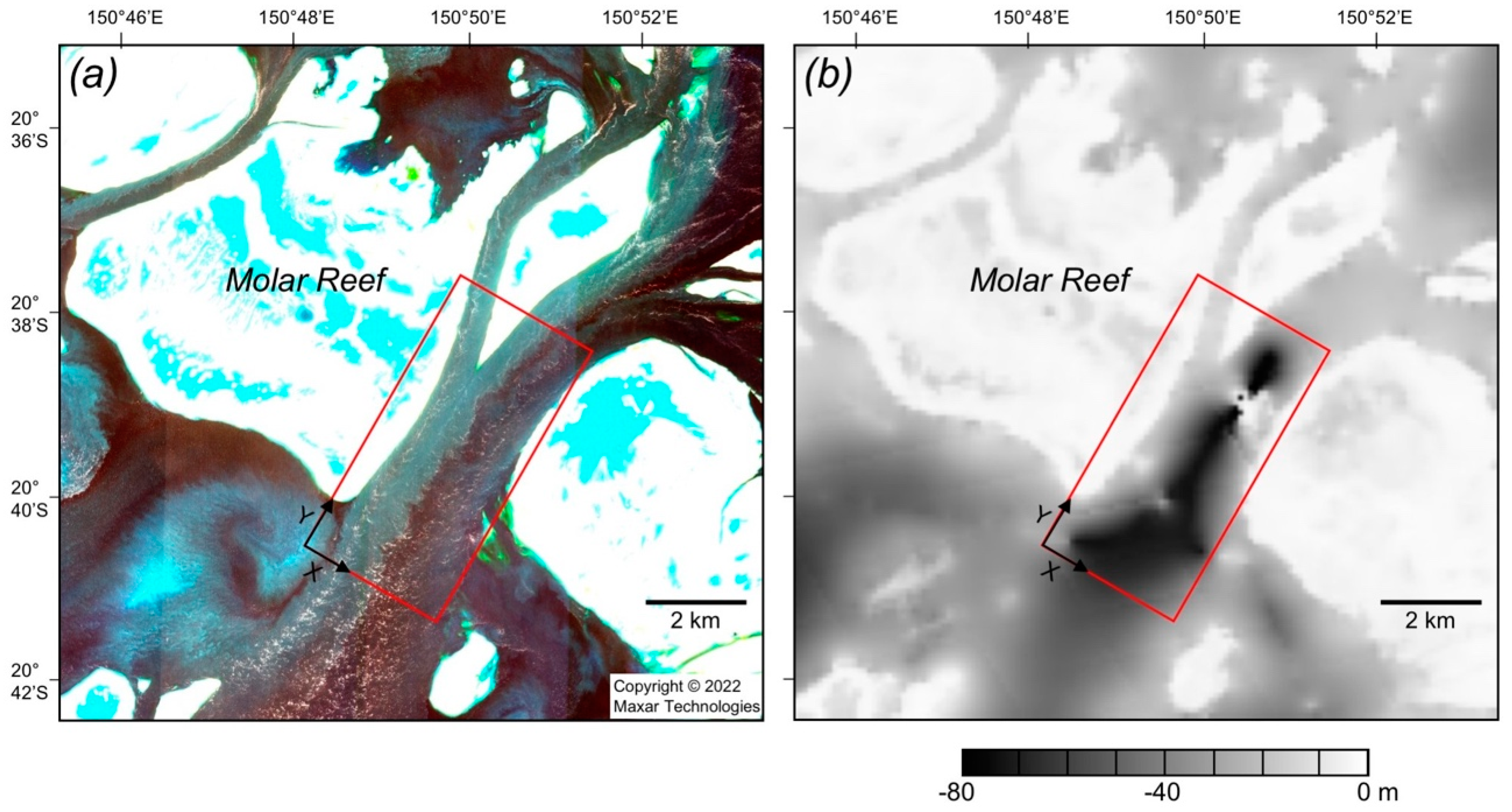
2.1. Study Area

Figure 1 is an historical LANDSAT-8 image showing the southern, outer part of the Great Barrier Reef, near the end of a flood tide. Material suspended in the water makes visible a variety of sub-mesoscale circulation patterns. In particular, one can see a number of mushroom-shaped features; these are propagating dipolar vortices, which stem from jet-like flows exiting the many passages or channels between the reefs. The focus of this study is the channel lying between two such reefs: Molar Reef (highlighted in the figure) and an un-named reef to the southeast.

2.2. Satellite Data

We will analyze high-resolution imagery of Molar Reef as acquired by the WorldView-2 satellite, a commercial Earth observation satellite (Maxar Technologies, Westminster, CO, USA) that collects data in eight visible and near-infrared wavelength bands and one panchromatic band. Imagery on two days—22 August 2020, and 4 September 2020—was collected as “multi look”, meaning as many looks as possible of an area are obtained during a single overpass of the satellite. Sampling details for the two data collections are given in

Table 1. Sampling details for WorldView-2 multi-look data collected on the two days examined in this study. Underlining indicates those looks analyzed in this study. The value Δt is the time difference between successive looks. GSD is Ground Sample Distance, or resolution size, of a single pixel on the ground; listed values are for the panchromatic wavelength band. The off-nadir angle is given by θ_nadir. Azimuth angles (ϕ) are measured from the satellite to either the ground target or the sun. Sun elevation angles were ~42.6° for 22 August and ~50.4° for 4 September. Note that local Australian Eastern Standard Time (AEST) is UTC plus ten hours.

Day [2020]	Look	Image Identification	Time [UTC]	Δt [s]	GSD [m]	θnadir [°]	ϕtarget [°]	ϕSun [°]
22 August	1	10300100ABD88300	23:36:33.4		1.31	51.8	237.6	50.9
22 August	2	10300100AC13F000	23:36:48.3	14.9	1.20	50.3	241.5	50.9
22 August	3	10300100AC305700	23:37:03.3	15.0	1.10	48.7	246.0	50.8
22 August	4	10300100ABBA8D00	23:37:16.7	13.4	1.03	47.3	250.5	50.8
22 August	5	10300100ACAA6D00	23:37:29.6	12.9	0.97	46.1	255.3	50.7
22 August	6	10300100AC18CF00	23:37:41.5	11.9	0.93	45.1	260.2	50.7
22 August	7	10300100AB2A2100	23:37:53.1	11.6	0.90	44.3	265.3	50.6
22 August	8	10300100ABB64A00	23:38:04.9	11.8	0.87	43.6	270.9	50.6
22 August	9	10300100AA923200	23:38:16.6	11.7	0.86	43.2	276.7	50.5
4 September	1	10300100AD454900	23:57:58.8		0.72	37.1	215.3	49.6
4 September	2	10300100AC053700	23:58:11.3	12.5	0.66	33.6	219.0	49.6
4 September	3	10300100ACB3D200	23:58:49.4	38.1	0.54	22.2	240.0	49.5
4 September	4	10300100AC2A0500	23:59:01.1	11.7	0.51	19.3	253.0	49.4
4 September	5	10300100AC9F1000	23:59:13.8	12.7	0.50	17.3	271.1	49.3
4 September	6	10300100ACBAA000	23:59:26.4	12.6	0.50	17.1	291.3	49.2
4 September	7	10300100A9504100	23:59:39.0	12.6	0.51	18.8	309.8	49.2

. Nine looks are available on 22 August, with values of time-lag Δt varying from 11.7 to 14.9 s. Seven looks are available on 4 September, all but one having a Δt value less than 13 s. For comparison, WorldView collections conducted as in-line stereo, as used in previous studies by the author, have Δt values in the range of 51 to 77 s [15,16]. Additional information about the data collections, including medium-resolution natural-color imagery, can be obtained by going to the online imagery archive (https://browse.digitalglobe.com/imagefinder/, accessed on 19 December 2021) and entering an image identification.

Image data were geo-referenced and resampled to a uniform UTM map grid at a spatial resolution of 2 m for the visible and near-infrared bands, and 0.5 m for the panchromatic band. Image quality on both days was affected by signals of atmospheric origin that move across the scene over time. These appear in the imagery as larger-scale bright and dark patches. This was more of an issue on 4 September, resulting in relatively poor image contrast in many looks; for this reason, only the two cleanest looks from that day are analyzed. Boil roughness signatures, being surface scatterers of sunlight, appear in all wavelength bands; but they were found to have the highest dynamic range in the “red edge” band, which corresponds to wavelengths in the range 706–746 nm. The red-edge data were thus chosen to be analyzed for currents (see below); sample panchromatic data are examined in Section 3.1.

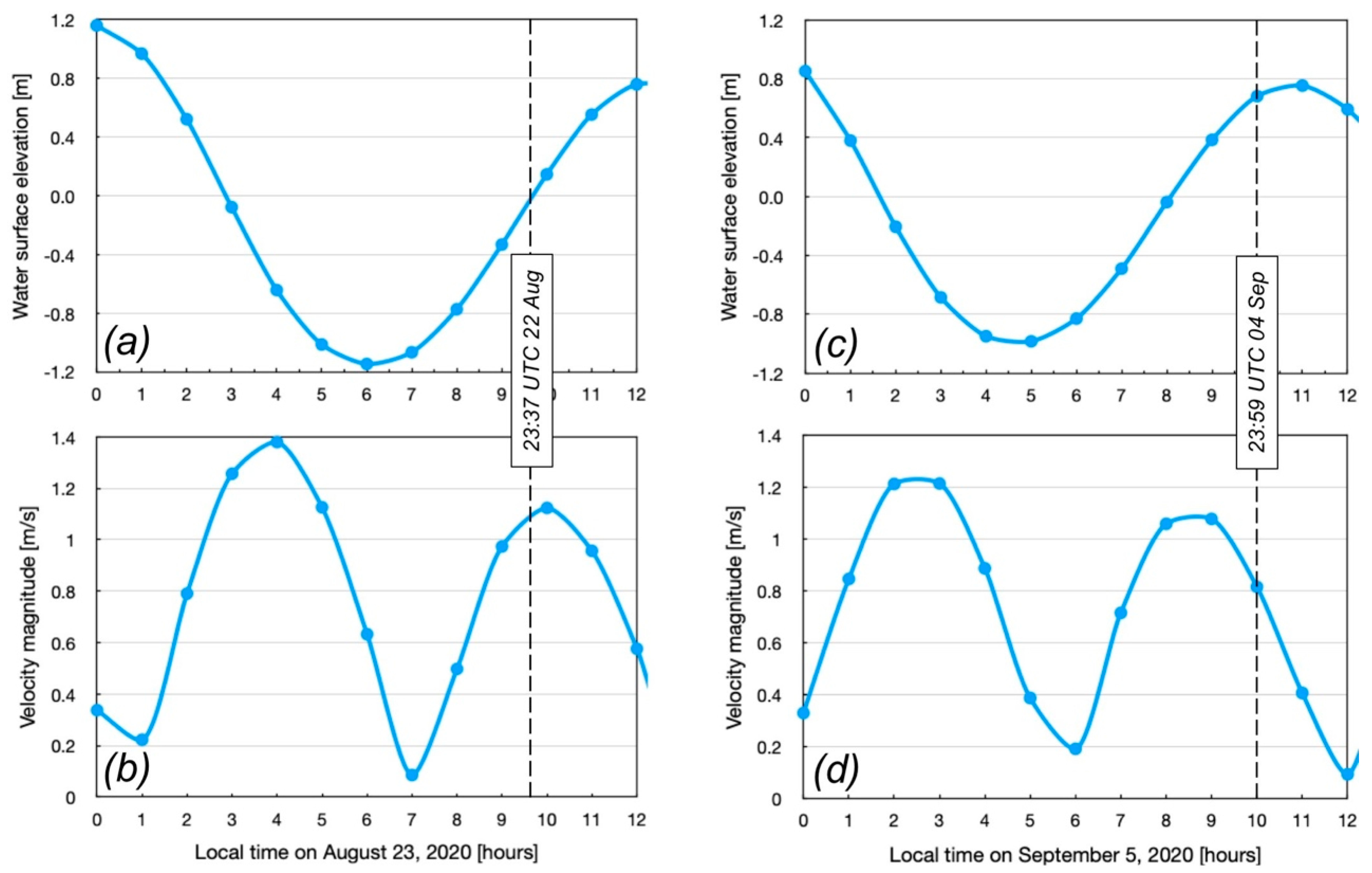
2.3. Molar Reef Environmental Conditions

A representative WorldView-2 image of Molar Reef from 22 August 2020 is shown in Figure 2, along with the corresponding bathymetry. The red rectangle in the figure indicates the area analyzed for currents. This area encompasses two relatively shallow (12 and 18 m depth) “entrance” channels in the north, and a more central main channel. At its widest, the main channel is 2.1 km across; it has a mean depth of about 42 m. A narrow underwater ridge appears to extend across the deep northern part of the main channel. The dominant color signature in the analysis area—the blue-green water along the western side—appears to derive from the outer margin of the reefs. The color signal is nearly uniform, consistent with a vertically well-mixed water column; thus, boils do not have a distinct color signature in this data set.

Predictions of water surface elevation and near-surface current speed for the study area are shown in Figure 3. These data derive from a hindcast archive of a hydrodynamic model of the Great Barrier Reef (https://research.csiro.au/ereefs/models/model-outputs/gbr1/, accessed on 19 December 2021). The model does not resolve the outer reef-channel bathymetry; so, data were extracted at the center of the Figure 2 study area, as representative of local conditions. It can be seen from Figure 3 that the collection on 22 August was achieved near the middle of flood tide, when the predicted surface current was near its maximum speed (for that particular flood tidal cycle) of about 1.1 m/s. The collection on 4 September was achieved near the end of a flood tide, when the predicted surface current is about 0.8 m/s. On both days the collections were made about three days after spring tide (not shown). Henceforth, these two collection periods will be referred to as mid-flood and late-flood cases.

Winds during the mid-flood collection were towards 355° at 9.5 m/s; during the late-flood collection, they were towards 313° at 5.3 m/s. These directions correspond to wind flow approximately along and across the main channel.

2.4. Deriving a Velocity Field from Image Pairs

Velocity vectors are derived from a particular pair of images using a normalized cross-correlation algorithm [18], which is implemented as a particle–image–velocimetry (PIV) “plugin” to the ImageJ processing and analysis package [19]. In this algorithm an n × n pixel-sized interrogation window in the first image is compared against a larger search area in the second image. The difference in center positions of the interrogation window and its best match within the search area is then selected as the displacement vector; the displacement vector divided by Δt yields the velocity vector. Each successive interrogation window is displaced in the x and y directions by n/2 pixels (i.e., a 50% spatial overlap); the resulting velocity vectors thus have a physical spacing of n/2 times the pixel size Δx. The choice of interrogation window size represents a trade-off between spatial resolution of the resulting velocity field and capturing sufficient spatial density of trackable features, or “particles”. The latter can be an especial difficulty when using a naturally occurring tracer, as in the present application, as there is often an uneven “seeding” of the flow field. In the present case, we use n = 128 and Δx = 2 m, giving an interrogation window of 256 m × 256 m. Examples of images of this exact size are shown in the following section, enabling the reader to see how much variation there can be in the density of features. We did, of course, experiment with the use of other window sizes. A smaller interrogation window produced unsatisfactory results: low values of peak correlation and a noisy vector field; a larger window resulted in too few vectors in the narrowest part of the analysis area.

3. Results

In this section, we first take a look at the nature of the boil signatures that are to be used as tracers; then, surface velocity fields are derived for both the mid-flood and late-flood cases.

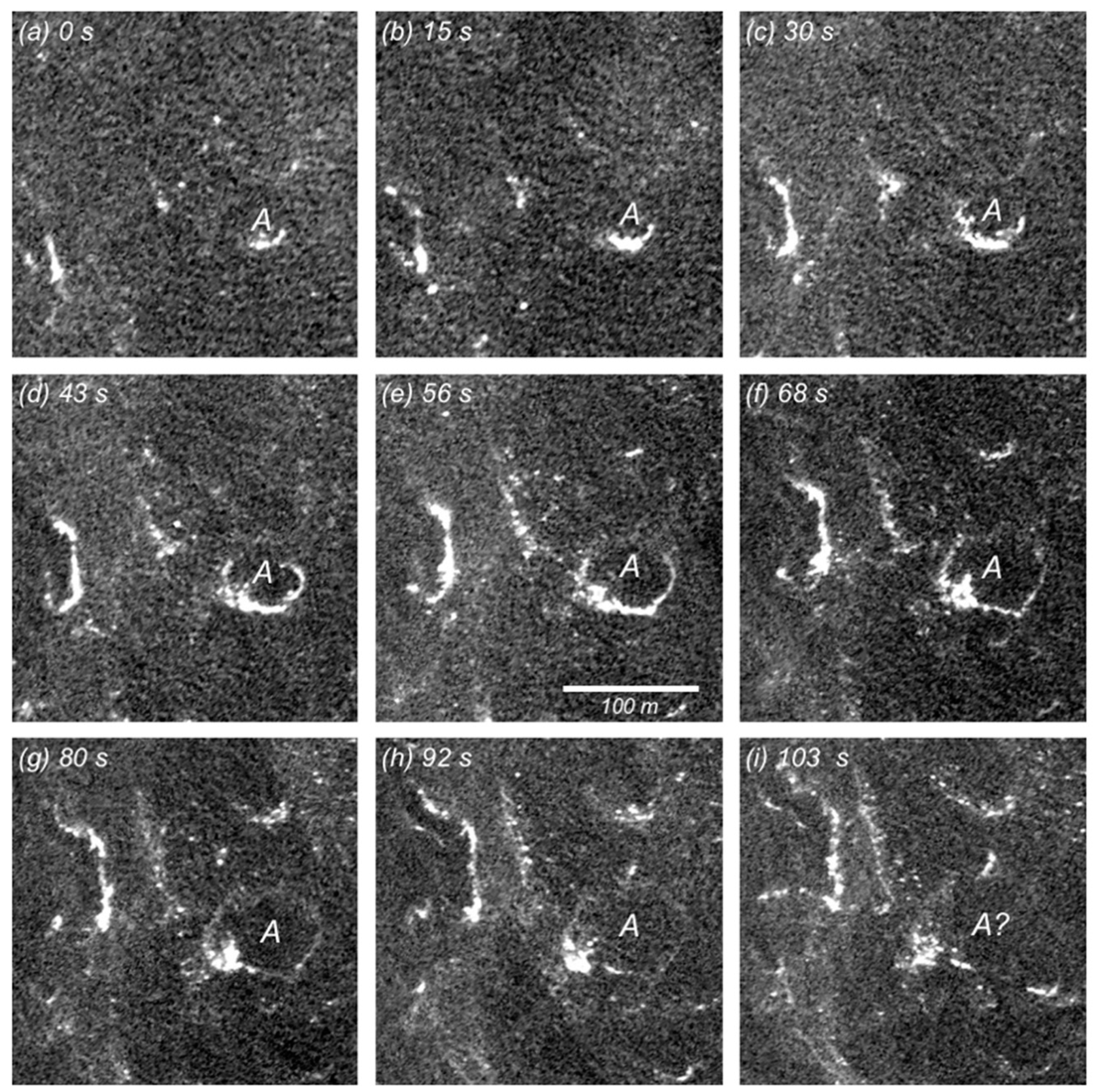
3.1. Nature of the Boil Signatures

Figure 4 shows, for the mid-flood case, nine looks at approximately the same area of ocean surface as it moves down the channel. The bright features in the figure are surface roughness signatures, i.e., enhanced scattering of sunlight from bubbles and foam from breaking waves. Feature “A” in the figure is an example of a boil that can be seen to grow and then to dissipate within the 103-s time window provided by the sequence of looks. It may be noted that the boil signatures in this dataset rarely develop as a complete ring of enhanced scattering; rather, most often there is only a partial, crescent-shaped signature. This is likely a result of the wind flow direction (approximately bottom-to-top in the Figure), as surface scattering features will preferentially develop along the part of the boil-induced convergence region facing into the wind–wave field [4]. Under the assumption that an expanding boil has an approximately circular shape, a boil area A can be estimated by fitting a circle to as much of the signature as is visible. By performing this for the boil highlighted in Figure 4, we find that its area increases approximately as dA/dt ~ 47 m²/s. This rate of area expansion can be used to estimate a radial surface velocity V_r = dr/dt = dA/dt/2π r, where r is the instantaneous radius of a boil. For example, at the time of Figure 4e, the boil radius is r ~ 30 m; thus, V_r ~ 0.25 m/s. This value is about 8% of the background surface flow speed (see below).

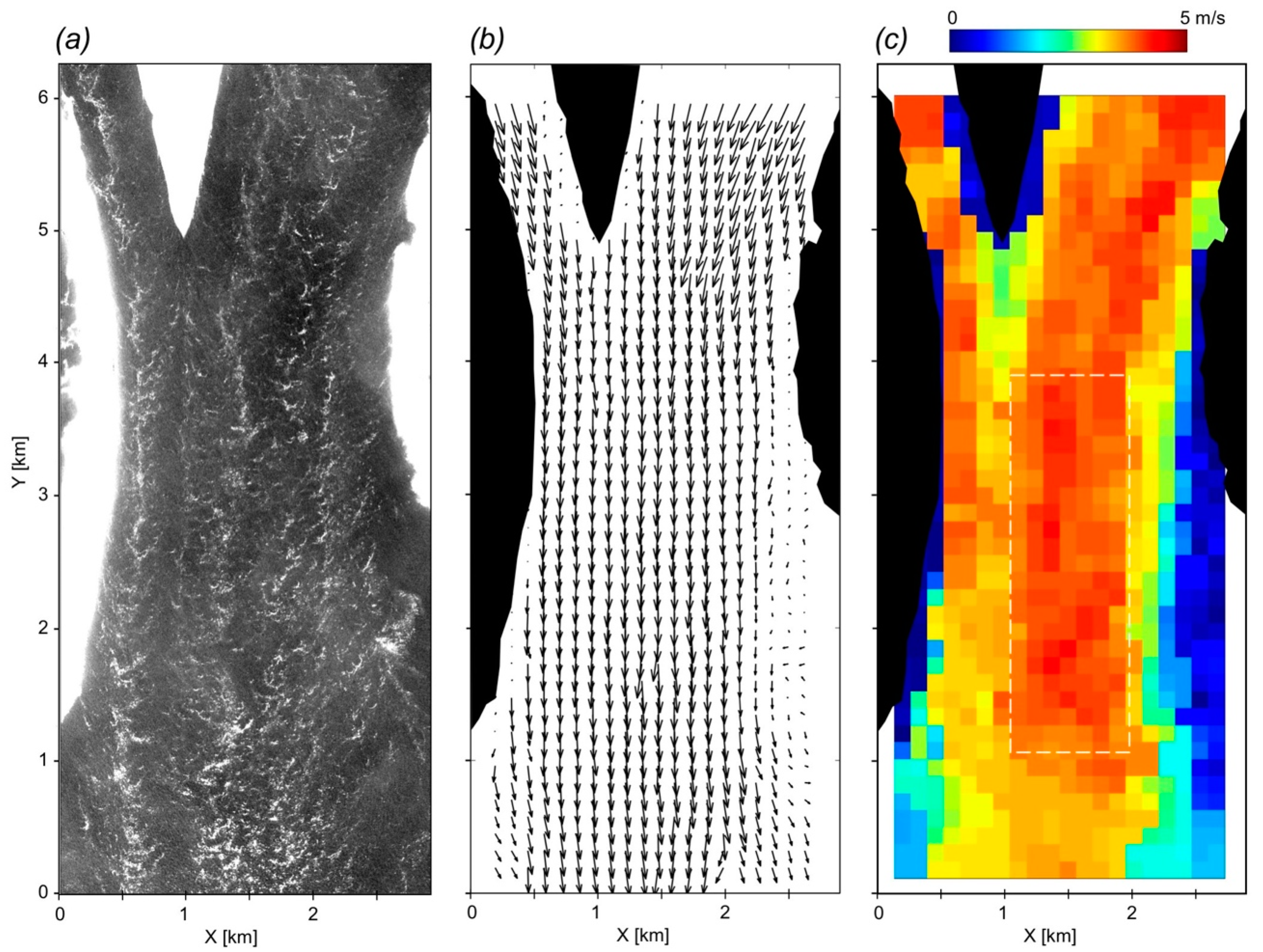
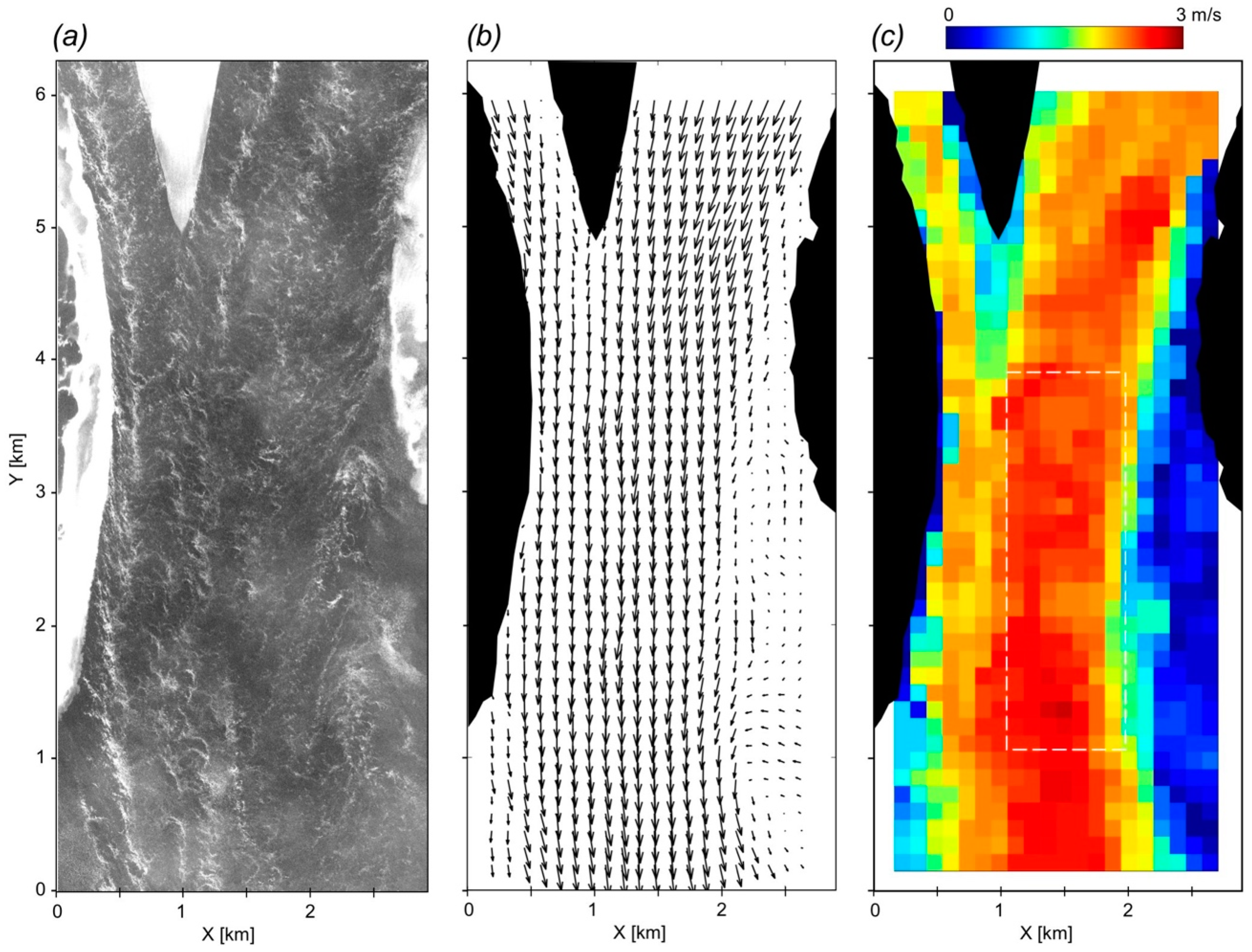
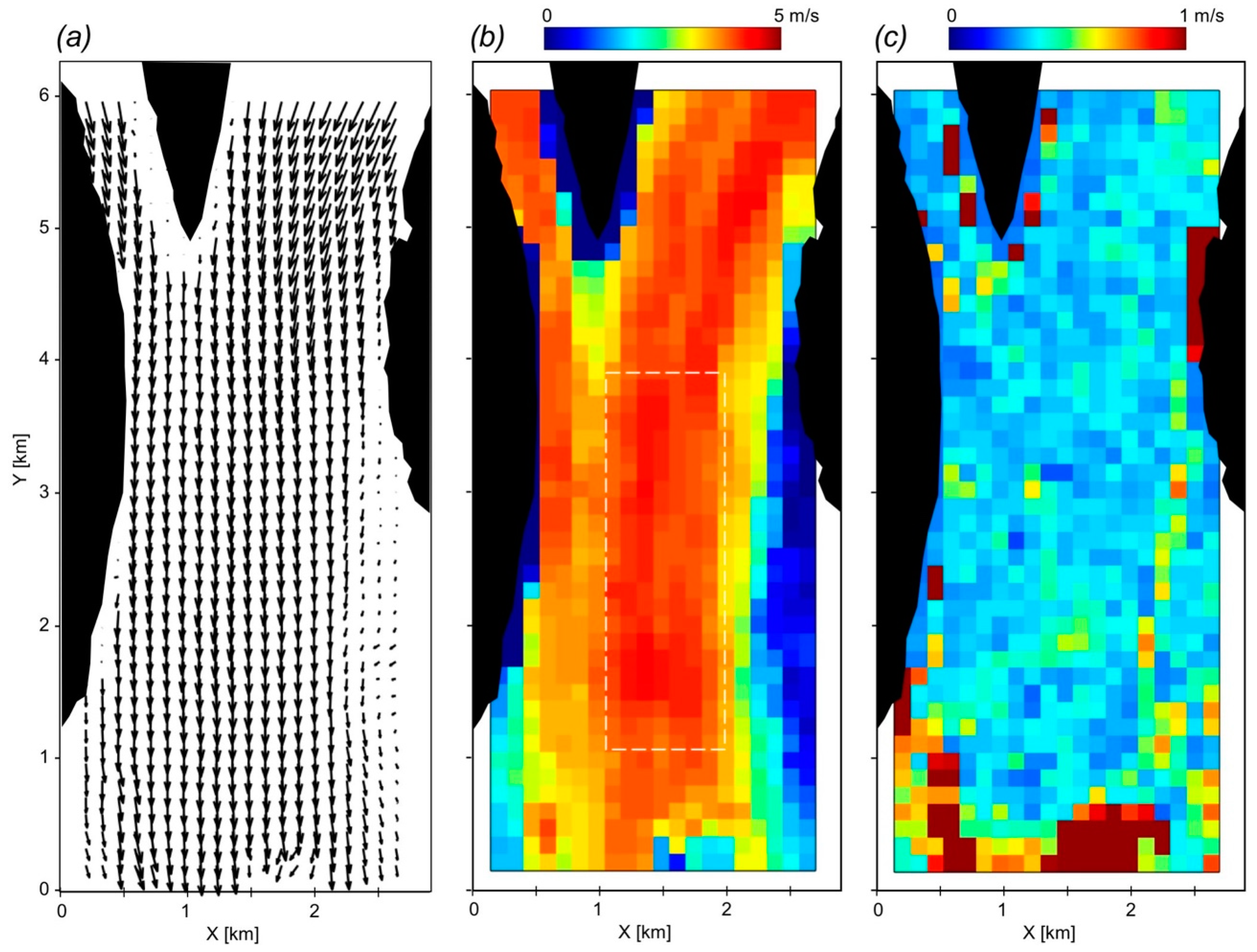
3.2. Surface Velocity Fields

A sample velocity field for the mid-flood case as derived from PIV analysis is shown in Figure 5. These results use looks 6 and 7 as an image pair, for which the time separation is Δt = t₂ − t₁ = 11.6 s (see Table 1). The derived flow is strongly guided by bathymetry, as one would expect. There is a nearly equally strong flow in the two shallow entrance channels, but the flow from the narrower entrance appears to hug the western boundary and not merge with the flow from the wider channel. A spatial average of the flow over the central part of the main channel (over the dashed rectangle in Figure 5c) yields a mean velocity magnitude of 3.92 m/s (±0.25 m/s), which is quite a large value. As the flow exits the reef channel, however, there is an apparent falloff in current speed (see below).

A velocity field for the late-flood case is shown in Figure 6. These results use looks 5 and 6 as the image pair; the time separation is Δt = t₂ − t₁ = 12.6 s. Compared with the mid-flood results, the overall flow speeds are less; this is consistent with weaker tidal forcing in late flood. Unlike the mid-flood case, flow in the narrowest channel and flow along the western reef edge are weaker than in the main channel; an effect we assume is related to the difference in tidal phase. Another difference is that in this late-flood example the flow maintains its high speed as it exits the main channel; even though the bathymetry widens there, the flow remains narrow, resembling an emergent jet-like current. However, in neither case is there a speeding up of the flow over the supposed bathymetric sill (Figure 2b). This suggests the bathymetry data may be in error at that location. In this late-flood case, a spatial average of the flow over the central part of the main channel yields a mean magnitude of 2.30 m/s (±0.27 m/s).

For the mid-flood case, PIV calculations were also done on the remaining seven pairs of consecutive looks, e.g., looks 1 and 2; 2 and 3, etc. Results from all eight calculations were then averaged to form an ensemble-averaged velocity field (Figure 7). Compared with the single realization of Figure 5, the ensemble vector and magnitude fields are smoother, as one would expect; however, still present is the fall-off in speed as the flow exits the reef channel. The main-channel ensemble mean magnitude is 3.81 m/s (±0.16 m/s), statistically the same as found for the single realization. The ensemble averaging also provides a measure of reliability for the mean flow field in the form of an rms (root-mean-square) map, which is shown as Figure 7c. Over most of the channel, rms values are ~0.3 m/s, or less. Very high values (in excess of 1 m/s) occur near the reef edge and where the exiting current flows into the open shelf water; the velocity field is thus suspect in such areas. So, taking the rms maps into account, the fall-off in the exit jet speed found the mid-flood results (Figure 5 and Figure 7) is probably spurious.

4. Discussion

In summary, velocity magnitudes within the main channel as derived from the imagery are as high as ~3.8 m/s at mid-flood and ~2.3 m/s at late-flood. There are no in situ measurements near the Molar Reef channel, but we can make comparisons with the literature from elsewhere within the Great Barrier Reef and with two supplementary analyses. From the literature, numerical modeling of flow through a dense area of reefs in the central part of the Great Barrier Reef shows currents in reef passages peaking at only 1.2 to 1.3 m/s during spring tides [20,21]; and the strongest tidal currents within channels of the Ribbon Reefs, which form the Great Barrier Reef’s northern outer reefs, are just over 1 m/s during flood tide [22,23]. These values are much smaller than the image-derived values of the present study.

While there are no directly relevant published data with which to compare, we can at least demonstrate that the large velocity values we report are not unique. This is achieved in a supplementary analysis by examining the channel on the other (northwest) side of Molar Reef, during mid-flood conditions as for Figure 5 and Figure 7. The northwest channel has a mean depth of about 15 m and a width of 450 m. The results (Figure S1) show currents exceeding 4 m/s over the middle stretch of the channel. Thus, image analysis shows strong flow on both sides of Molar Reef. One can speculate, then, that strong currents occur in other channels within the outer reef complex.

A skeptic might say, however, that there yet may be some systematic error that is causing very large currents. To address this possibility, we did a second supplemental analysis that examines an “ambient” area of dipolar vortices located about 10 km inshore of Molar Reef (Figure S2). Again, we use data from the mid-flood case. The PIV results are shown in Figure S3. In this case, we aim to minimize the influence of light back-scattered from the sea surface, as we need to trace out the small-scale sediment features stirred upward by the vortices; hence, data from the water-penetrating band 3 (wave lengths of 518 to 586 nm) are analyzed. Additionally, because the ambient currents are expected to be weaker, an image pair having longer time separation (Δt = 50 s) is used; this also helps de-correlate the surface scatter. Again, there are no in situ data, but the pattern of the resulting velocity field with respect to the tri-polar structure evident in the imagery makes sense; and the magnitude of the vorticity cores (~0.001 s⁻¹) and of the velocity (~0.6 m/s) are consistent with the characteristics of similarly sized vortices studied by Delandmeter et al. [2]. In that study, a WorldView-3 image having Δt=54 s was analyzed and compared (favorably) with high-resolution simulations using the unstructured-mesh, finite-element model SLIM. Thus, these additional results suggest there is no systematic error in our analysis.

5. Conclusions

The present study has demonstrated that multiple satellite images acquired quite closely in time can be used to derive a plausible spatial map of the surface current in situations where the near-surface hydrodynamics are dominated by bed-generated turbulence and associated wave-current interaction. The approach was illustrated using imagery of turbulent tidal flow in a channel through the outer part of the Great Barrier Reef. The results show velocity magnitudes of nearly 4 m/s during a flooding tide—three times larger than published values for passages elsewhere in the Reef. Further comparison of image-derived velocity fields and high-resolution ocean models are warranted. Of particular interest would be the forcing of the rich sub-mesoscale field of vortices that lies inshore of the outer reefs, and which affects the transport of tracers and particles, and which impacts marine ecology [24].

References

1. Qazi, W.A.; Emery, W.J.; Fox-Kemper, B. Computing ocean surface currents over the coastal California current system using 30-min-lag sequential SAR images. IEEE Trans. Geosci. Remote Sens. 2014, 52, 7559–7580. [Google Scholar] [CrossRef]
2. Delandmeter, P.; Lambrechts, J.; Marmorino, G.O.; Legat, V.; Wolanski, E.; Remacle, J.F.; Chen, W.; Deleersnijder, E. Submesoscale tidal eddies in the wake of coral islands and reefs: Satellite data and numerical modelling. Ocean Dyn. 2017, 67, 897–913. [Google Scholar] [CrossRef]
3. Nimmo Smith, W.A.M.; Thorpe, S.A.; Graham, A. Surface effects of bottom-generated turbulence in a shallow tidal sea. Nature 1999, 400, 251–254. [Google Scholar] [CrossRef]
4. Thorpe, S.A.; Green, J.A.M.; Simpson, J.H.; Osborn, T.R.; Smith, W.N. Boils and turbulence in a weakly stratified shallow tidal sea. J. Phys. Oceanogr. 2008, 38, 1711–1730. [Google Scholar] [CrossRef]
5. Marmorino, G.; Chen, W.; Mied, R.P. Submesoscale Tidal-Inlet Dipoles Resolved Using Stereo WorldView Imagery. IEEE Geosci. Remote Sens. Lett. 2017, 14, 1705–1709. [Google Scholar] [CrossRef]
6. Chickadel, C.C.; Horner-Devine, A.R.; Talke, S.A.; Jessup, A.T. Vertical boil propagation from a submerged estuarine sill. Geophys. Res. Lett. 2009, 36, L10601. [Google Scholar] [CrossRef] [Green Version]
7. Marmorino, G.O.; Smith, G.B.; Miller, W.D. Surface imprints of water-column turbulence: A case study of tidal flow over an estuarine sill. Remote Sens. 2013, 5, 3239–3258. [Google Scholar] [CrossRef] [Green Version]
8. Slingsby, J.; Scott, B.E.; Kregting, L.; McIlvenny, J.; Wilson, J.; Couto, A.; Roos, D.; Yanez, M.; Williamson, B.J. Surface Characterisation of Kolk-Boils within Tidal Stream Environments Using UAV Imagery. J. Mar. Sci. Eng. 2021, 9, 484. [Google Scholar] [CrossRef]
9. Lieber, L.; Langrock, R.; Nimmo-Smith, W.A.M. A bird’s-eye view on turbulence: Seabird foraging associations with evolving surface flow features. Proc. R. Soc. B 2021, 288, 20210592. [Google Scholar] [CrossRef]
10. Longuet-Higgins, M.S. Surface manifestations of turbulent flow. J. Fluid Mech. 1996, 308, 15–29. [Google Scholar] [CrossRef]
11. Fujita, I.; Komura, S. Application of video image analysis for measurements of river-surface flows. Proc. Hydraul. Eng. 1994, 38, 733–738. [Google Scholar] [CrossRef]
12. Fujita, I.; Hino, T. Unseeded and seeded PIV measurements of river flows videotaped from a helicopter. J. Vis. 2003, 6, 245–252. [Google Scholar] [CrossRef]
13. Legleiter, C.J.; Kinzel, P.J. Inferring Surface Flow Velocities in Sediment-Laden Alaskan Rivers from Optical Image Sequences Acquired from a Helicopter. Remote Sens. 2020, 12, 1282. [Google Scholar] [CrossRef] [Green Version]
14. Legleiter, C.J.; Kinzel, P.J. Surface flow velocities from space: Particle image velocimetry of satellite video of a large, sediment-laden river. Front. Water 2021, 3, 53. [Google Scholar] [CrossRef]
15. Marmorino, G.O.; Smith, G.B.; Miller, W.D. Turbulence characteristics inferred from time-lagged satellite imagery of surface algae in a shallow tidal sea. Cont. Shelf Res. 2017, 148, 178–184. [Google Scholar] [CrossRef]
16. Marmorino, G.; Chen, W. Use of WorldView-2 along-track stereo imagery to probe a Baltic Sea algal spiral. Remote Sens. 2019, 11, 865. [Google Scholar] [CrossRef] [Green Version]
17. Beaman, R.J. Project 3DGBR: A High-Resolution Depth Model for the Great Barrier Reef and Coral Sea. Marine and Tropical Sciences Research Facility (MTSRF) Project 2.5i.1a Final Report; MTSRF: Cairns, Australia, 2010; pp. 1–13. [Google Scholar]
18. Tseng, Q.; Duchemin-Pelletier, E.; Deshiere, A.; Balland, M.; Guillou, H.; Filhol, O.; Théry, M. Spatial organization of the extracellular matrix regulates cell–cell junction positioning. Proc. Nat. Acad. Sci. USA 2012, 109, 1506–1511. [Google Scholar] [CrossRef] [Green Version]
19. Schneider, C.A.; Rasband, W.S.; Eliceiri, K.W. NIH Image to ImageJ: 25 years of image analysis. Nat. Methods 2012, 9, 671–675. [Google Scholar] [CrossRef]
20. Wolanski, E.; Spagnol, S. Sticky waters in the Great Barrier Reef. Estuar. Coast. Shelf Sci. 2000, 50, 27–32. [Google Scholar] [CrossRef] [Green Version]
21. Andutta, F.P.; Kingsford, M.J.; Wolanski, E. ‘Sticky water’ enables the retention of larvae in a reef mosaic. Estuar. Coast. Shelf Sci. 2012, 101, 54–63. [Google Scholar] [CrossRef] [Green Version]
22. Wolanski, E.; Drew, E.; Abel, K.M.; O’Brien, J. Tidal jets, nutrient upwelling and their influence on the productivity of the alga Halimeda in the Ribbon Reefs, Great Barrier Reef. Estuar. Coast. Shelf Sci. 1988, 26, 169–201. [Google Scholar] [CrossRef]
23. Young, I.R.; Black, K.P.; Heron, M.L. Circulation in the ribbon reef region of the Great Barrier Reef. Cont. Shelf Res. 1994, 14, 117–142. [Google Scholar] [CrossRef]
24. Wolanski, E.; Pickard, G.L. Physical Oceanographic Processes of the Great Barrier Reef; CRC Press: Boca Raton, FL, USA, 2018. [Google Scholar]
Figure 1. Historical LANDSAT-8 image of a part of the Great Barrier Reef, showing flow circulation patterns made visible by material suspended in the water. The image was collected near the end of a flood tide on 23 August 2013, at 00:01 UTC. The focus of the present study is Molar Reef, which is labeled.
Remotesensing 14 00783 g001
Figure 2. (a) Molar Reef as seen by the WorldView-2 satellite at 23:37 UTC 22 August 2020. Shown are data from bands 5, 3, and 2 (red, green, and blue wave lengths) but the color ranges have been stretched to reveal both water surface scattering and water color changes across the channel. Red rectangle shows the analysis area, which is aligned with the main channel between Molar Reef and the unnamed reef lying to the southeast. (b) Bathymetry has 100-m spatial resolution [17]. Scale bar indicates depth in meters.
Remotesensing 14 00783 g002
Figure 3. Predictions of water surface elevation and surface current speed coinciding with WorldView-2 data collected at 23:37 UTC 22 August 2020 (a,b) and 23:59 UTC 4 September 2020 (c,d), as indicated by the two dashed, vertical lines. Data shown were extracted from the “ereefs” model archive at the center of the study area shown in Figure 2.
Remotesensing 14 00783 g003
Figure 4. Example of the evolution of a boil (feature “A”) over time. (ai) Approximate Lagrangian views of the same area of water surface, as captured in nine consecutive looks from the mid-flood case (Table 1, 22 August 2020). Times shown are relative to look 1; data are from the panchromatic band. Each panel has a size of 256 m by 256 m, which is the same size as the interrogation window used in the PIV calculations. Local water depth is 36 m.
Remotesensing 14 00783 g004
Figure 5. Velocity field at mid-flood as derived from PIV analysis of an image pair (looks 6 and 7) having a time separation of Δt = t2t1 = 11.6 s (see Table 1). (a) Red-edge imagery at time t1; (b) velocity vectors; (c) velocity magnitude. Black areas are a land mask. The longest vector in (b) has a length of 4.37 m/s. Dashed rectangle in (c) shows area used for spatial averaging.
Remotesensing 14 00783 g005
Figure 6. Velocity field at late-flood as derived from PIV analysis of an image pair (looks 5 and 6) having a time separation of Δt = t2t1 = 12.6 s. (a) Red-edge imagery at time t1; (b) velocity vectors; (c) velocity magnitude. Large, relatively bright and dark patches in the imagery are atmospheric artifacts. The longest vector in (b) has a length of 2.83 m/s. Note that the magnitude scaling differs from Figure 5, as the upper limit here is only 3 m/s.
Remotesensing 14 00783 g006
Figure 7. Ensemble-averaged result for mid-flood case: (a) Velocity vectors; (b) velocity magnitude; (c) root-mean-square values. The results derive from PIV analyses of eight consecutive image pairs (see Table 1, 22 August 2020).
Remotesensing 14 00783 g007