Article

Coupling Data- and Knowledge-Driven Methods for Landslide Susceptibility Mapping in Human-Modified Environments: A Case Study from Wanzhou County, Three Gorges Reservoir Area, China

1
Faculty of Engineering, China University of Geosciences, Wuhan 430074, China
2
School of Geography and Information Engineering, China University of Geosciences, Wuhan 430078, China
3
Research Center of Geohazard Monitoring and Warning in the Three Gorges Reservoir, China University of Geosciences, Chongqing 404100, China
4
Department of Civil Engineering and Architecture, University of Catania, 95125 Catania, Italy
*
Author to whom correspondence should be addressed.
Remote Sens. 2022, 14(3), 774; https://doi.org/10.3390/rs14030774
Submission received: 29 December 2021 / Revised: 26 January 2022 / Accepted: 1 February 2022 / Published: 7 February 2022

Abstract

:
Landslide susceptibility mapping (LSM) can provide valuable information for local governments in landslide prevention and mitigation. Despite significant improvements in the predictive performance of LSM, it remains a challenge to be carried out in areas with limited availability of data. For example, in the early stage of road construction, landslide inventory data can be particularly scarce, while there is a high need to have a susceptibility map. This study aims to set up a novel procedure for coupling the knowledge-driven and data-driven models for LSM in an area with limited landslide inventory data. In particular, we propose a two-step approach. The first step consists of applying four data-driven models (logistic regression, decision tree, support vector machines, and random forest (RF)) to derive a regional susceptibility map. In the second step, the application of a heuristic model (analytic hierarchy process, AHP) is proposed to calculate a local susceptibility map for the areas with incomplete landslide inventories. The final landslide susceptibility map is obtained by merging the most accurate regional map (RF) with the local map. We apply this novel procedure to a landslide-prone region with developed road construction (National Highway G69) in Wanzhou district, where landslide inventory is difficult to update due to timely recovery from landslide-induced road damage. Results show that the proposed methodology allows identifying new landslide-prone areas, and improving LSM predictive performance, as demonstrated by the fact that two new landslides developed along G69 were perfectly classified in the highly susceptible areas. The results show that implementing the landslide susceptibility assessment with different geographical settings and combining them into best-sensitivity partitions is more accurate than focusing on creating new models or hybrid models.

1. Introduction

Landslides pose great threats to human lives and economic development around the world [1]. The mountainous areas of southwestern China suffer a lot from landslide hazards. For instance, the Shuicheng landslide-debris occurred in Guizhou Province, China, resulting in 21 buildings being buried, 9 missing people, and 42 deaths in 2019 [2]. Another catastrophic landslide in Jiweishan Mountain, Chongqing province, China, caused 79 deaths in 2009 [3].
Landslide susceptibility is a spatial probability of an area to the future occurrence of landslides [4,5]. It predicts “where” landslides are likely to occur, which is the foundation of landslide early warning and risk assessment. A variety of methods have been proposed to ascertain landslide susceptibility. Essentially, most of the approaches and methods are based upon the assumption that slope instability is more likely to occur under the conditions that already led to landslides in the present and past [1].
Characterising the spatial pattern of landslide occurrence and improving the accuracy of landslide susceptibility mapping (LSM) are difficult missions. To date, the landslide susceptibility models can be divided into four categories: inventory-based methods, physically based models, heuristic models, and data-driven models [6]. When the landslide inventory data are limited, we can use heuristic models based on expert knowledge of landslide deformation mechanisms [7,8]. With the fast development of geographic information systems (GISs) and soft computing techniques, many advanced data-driven models have been proposed to conduct LSM [9]. The data-driven models can be mainly divided into statistic models and machine learning (ML) models [10]. The statistical model includes an information value model [11] and logistic regression (LR) [12], while the ML model includes artificial neural networks [13,14], decision tree (DT) [15,16], support vector machine (SVM) [17,18], and random forest (RF) [19], etc. The present scientific literature reports that ML models perform very well in many research areas due to their mathematical flexibility [1,20]. Although nonlinear correlations between landslide and related conditioning factors can be efficiently fitted and predicted by data-driven models, the assessment accuracy is very reliant on the completeness of the landslide inventory.
At present, a reliable landslide inventory can be obtained by many advanced remote sensing techniques. One of these techniques is Interferometric Synthetic Aperture Radar, etc. [21,22]. Nevertheless, due to some inherent limitations, such as dense vegetation and climate and land change, in many cases, landslides are difficult to spot. Missing landslide inventory data affected the accuracy of LSM obtained by data-driven models. In hilly areas, slope-cutting is inevitable during the road-construction period. Slope-cutting often alters the original stress balance of the natural slope [23,24], which in turn leads to the fracture of the rock mass structure in the unloading area, the exposure of weak layers, and so on. Therefore, the land modifications caused by road construction often increase the frequency of landslides occurrence [25,26]. More often than not, slope-cutting-induced landslides do not occur immediately but instead are due to progressive failure progress due to the long-term action of dynamic loads of the road, rainfall, etc.
In mountainous areas, in order to meet the functional requirements of the road, most of the slope-cutting induced sliding mass along the road are recovered timely. This makes it challenging to build an accurate and significant landslide inventory that can be effectively used for LSM and opens the need to propose novel landslide susceptibility mapping procedures that allow operating in situations of incomplete landslide inventories.
Given the above issues, in this study, we propose a novel procedure to assess landslide susceptibility in areas with incomplete landslide inventories. The procedure couples data-driven and knowledge-driven approaches. A landslide-prone region with slope-cutting caused by road construction in Wanzhou District was selected as a case study. Four data-driven models (LR, DT, SVM, RF) and heuristic models (analytic hierarchy process) were combined to predict landslide susceptibility of the whole region and the area along National Highway G69, respectively. We produced the final landslide susceptibility map by merging the most accurate regional landslide susceptibility map with the road-affected landslide susceptibility map. Where susceptibility zonation is prepared for land planning, early warning or other practical applications, the authors hoped that the proposed two-step procedure could complete a more accurate susceptibility map to reduce the economic damage and human losses coursed by landslide hazards.

2. Study Area

The study area is located in Wanzhou County, the southwestern of China (108°17′47″ E~108°21′35″ E in longitude and 30°32′02″ N~30°34′36″ N in latitude) (Figure 1). It is composed of hills and mountains (up to 770 m of the elevation) with an area of 12.9 km2. Wanzhou belongs to the subtropical monsoon area, with an average annual rainfall of 1191 mm. The roads in the study area are well developed, and the newly built important traffic line, G69 national highway, runs through the whole area (Figure 1c). After field investigations, a 50-m buffer zone of G69 was selected as the target area for the road-affected LSM (this area is herein referred to as “G69”).
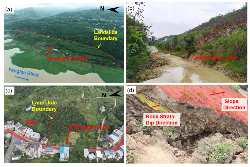
In this study area, as the distance from the Yangtze River increases, the exposed bedrock becomes older. Bedrock mostly formed during the Mesozoic Triassic and Jurassic from 137 to 250 Ma. The rock stratum tilts west in general, and the dip angle of the rock stratum gradually decreases to nearly horizontal from the mountain to the Yangtze River (Figure 1d). In addition, the rock strata dip is nearly perpendicular to the flow direction of the Yangtze River, with an average dip angle of 15° [27]. The fluctuation of the reservoir water level, rainfall and hill-cutting are the crucial triggering factors of landslide occurrence. For example, the Jinjinzi landslide was triggered by heavy rainfall and the rapid drawdown of reservoir water level (Figure 2a), while the Tongzilin landslide was induced by slope-cutting during construction activities (Figure 2c). The rock strata of the Tongzilin landslide have the same attitude as the slope surface.

3. Methodology

3.1. Modelling Algorithms

3.1.1. Information Value Model

The information value (IV) model can usefully calculate the importance of landslide causal factors, and the larger IV, the more important for landslide occurrence [11]. Assuming that landslide occurrence (y) is affected by various factors ( x 1 , x 2 x n ), the formula for IV can be written as:
I y , x 1 , x 2 x n = i = 1 n I i = i = 1 n log 2 S 0 i / S i A 0 / A ,
where I y , x 1 , x 2 x n is the IV under the landslide causal factor, Ii is the IV of factor x 1 , A is the total area, A0 is the area under the factor x 1 , S is the total area of landslides, and S0 is the area of landslides under the factor x 1 .

3.1.2. Logistic Regression

Logistic regression (LR) is a widely employed regression algorithm [13]. High calculation speed is among its advantages. In the application of LSM, the learning goal of the LR model is to quantitatively describe the relationship between the occurrence probability of a landslide and its causative factors. The calculation formula of LR can be expressed as:
y ( x ) = 1 1 + e θ T x ,
where the independent variable x refers to the factors that may cause landslides, such as altitude, slope, and aspect. The dependent variable y is landslide susceptibility index returned by LR, with a range of (0,1) [14].

3.1.3. Decision Tree

The decision tree (DT) model is widely used for prediction tasks and consists of tree growth, tree pruning, and boosting steps [15,16]. It works by splitting the sample based on the field that provides the maximum information gain. DT model represents the conditional probability distribution of the landslide occurrence or non-landslides under the conditions of given factors. The main advantage is that its classification is fast and easy to understand.

3.1.4. Random Forest

Random forest (RF) is a representative Bagging ensemble algorithm based on the decision tree as the evaluator, following the principle of average or minority to the majority to determine the ensemble result [28,29]. The higher the accuracy of a single decision tree, the higher the accuracy of the RF. Many studies show that the RF model provides a more effective ability to avoid over-fitting problems and generally achieves better generalisation performance than other ML techniques [1]. The performance of the RF model is mainly controlled by the number of trees in the forest N, the number of random factors M employed in each random tree, and the parameters of the maximum depth and a minimum number of samples. This study applies the grid optimisation function to select the optimal parameter combination.

3.1.5. Support Vector Machine

Support vector machine (SVM) is one of the algorithms that attracts most people’s attention in the ML [30]. The learning goal of SVM model is to find the separation hyperplane in the feature space, which can classify the training data set in the feature space into different classes. Radial Basis Function was selected to establish the SVM model in LSM.

3.1.6. Analytic Hierarchy Process

The analytic hierarchy process (AHP) is a semi-quantitative decision-making method of subjective weight assignment [31]. It adopts the simplification strategy of complex problems layer by layer and determines the weight of complex index systems through pairwise comparison. AHP model includes four steps: (a) decomposing the complex problems to be solved into components at different levels; (b) arranging causal factors hierarchically and establishing a hierarchical relationship model among indicators; (c) establishing a judgment matrix based on the important relationship between each index and verifying its rationality; (d) calculating the maximum eigenvalue of the judgment matrix, and giving the index weight in the corresponding level.

3.2. Proposed Framework for LSM

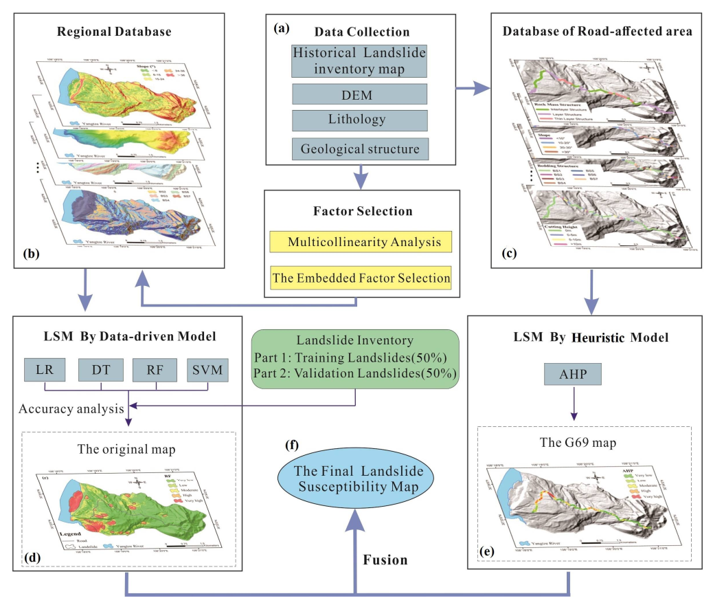
In this study, a procedure coupling heuristic and data-driven models was used to obtain high-quality landslide susceptibility map in complex geographic setting. This procedure includes the following six stages (Figure 3): (a) collect data required for LSM, including historical landslides data and a suite of landslide causal factors; (b) select the landslide causal factors for regional modelling, and construct a regional geospatial database with collected historical landslides; (c) construct a geospatial database of road-affected area, which including the causal factors of landslides developed under the slope-cutting conditions; (d) producing the preliminary landslide susceptibility map based on data-driven model; (e) generating the landslide susceptibility map of the road affected area (G69) by heuristic model based on expert knowledge; (f) producing the final susceptibility map by coupling the two landslide susceptibility maps of steps d and e.

4. Data Preparation

4.1. Regional Geospatial Database

4.1.1. Landslide Inventory

An accurate landslide inventory map can boost the understanding of the relationship between historical landslides distribution and landslide causal factors. Through field surveys and historical data collection, we built an inventory of 23 recorded landslide events with the attribution of location, type, boundary, material, and deformation characteristics. The landslide sizes range from 9987 m2 to over 482,976 m2, which covers 9.7% of the total area.

4.1.2. Landslide Conditioning Factors

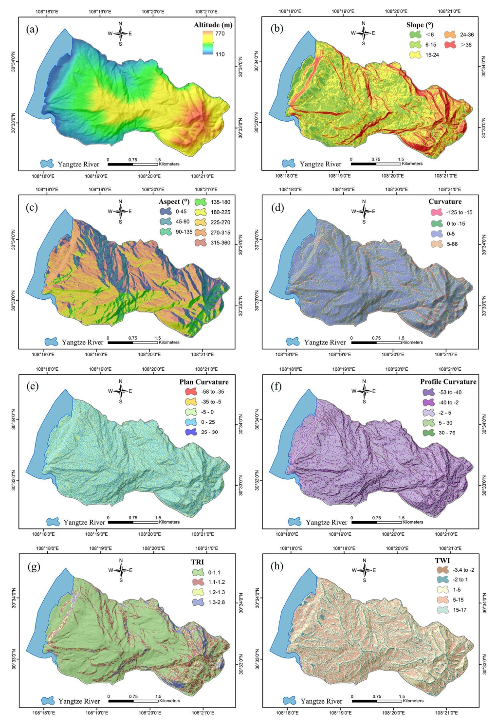
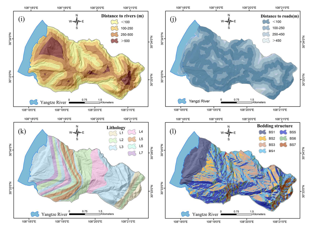
Based on the field survey and previous studies [32,33,34], 12 factors were initially selected for LSM in this paper, namely altitude, slope, aspect, curvature, plan curvature, profile curvature, topographic wetness index (TWI) [35], terrain roughness index (TRI) [36], lithology, bedding structure [37], distance to rivers, and distance to roads (Figure 4). Altitude, slope, aspect, curvature, TWI, and TRI were obtained by digital elevation model (DEM). Distance to rivers and distance to roads were calculated from the Euclidean distance analysis tool. Lithology and bedding structures were provided by the modified geological map. All the processing of factors in this research were conducted in ArcGIS 10.6 software.
Before modelling, landslide conditioning factors should be classified and normalised [19]. In this study, the method proposed by Yu et al. [37] was selected to discretise the continuous factors; after that, all factors were normalised between 0.01 and 0.99 based on the IV model. Finally, all the factors were divided into 5~8 classes (Table 1). The lithology was divided into seven classes: limestone and dolomite rock (L1), mudstone (L2), sandstone (L3), sandstone with mudstone (L4), shale with dolostone (L5), mudstone with silty mudstone (L6), and sand–mud interbed (L7). According to the China Geological Survey, bedding structure can be classified into eight categories: horizontal strata slope (BS1), over-dip slope (BS2), under-dip slope (BS3), dip-oblique slope (BS4), transverse slope (BS5), anaclinal oblique slope (BS6), and anaclinal slope (BS7) [37]. All indicator layers were converted into a 10 m spatial resolution raster format as independent variables in preparation for spatial modelling.

4.2. Geospatial Database of G69

At the G69 region, there are no data on historical landslides induced by slope cutting. Based on the knowledge of Geotechnics and Rock Mechanics, we selected six assessment factors for modelling, including slope, bedding structure, rock association, rock mass structure, cutting height, and overburden thickness. Slope and bedding structure are the same factor of the regional database, while slope refers to the natural slope angle before cutting. Cutting height refers to the height of the slope surface formed after the excavation of the slope foot when the road is constructed, which is a decisive factor in controlling the stability of the slope. Rock mass structure refers to the spatial spread of structural surfaces in a rock mass and their combination characteristic [23]. In addition, rock association is one of the factors which reflect the structural characteristics of slopes [38].
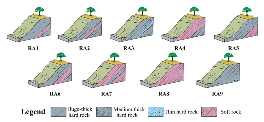
The cutting height data along the road were obtained by linear interpolation of the survey points. They were divided into 0 m, 0~5 m, 5~10 m, 10~20 m, and >20 m, respectively (Figure 5). Similarly, the collected data were interpolated by kriging to obtain the overburden thickness, which was divided into four categories: <0.5 m, 0.5~1 m, 1~1.5 m, and >1.5 m, respectively. The rock mass was classified into a blocky structure, layer structure, thin layer structure, interlayer structure, fragmented structure, and scattered structure [23]. The rock association is divided into nine categories by combining the distribution characteristics of soft layer location (Figure 6).

5. Results

5.1. Regional Landslide Susceptibility Modelling

5.1.1. Factor Selection

Multicollinearity Analysis

Numerous studies have contended that eliminating collinearity factors can improve the accuracy of LSM [39,40]. In this paper, the variance inflation factors (VIF) and the tolerances were used to quantify the correlation between landslide causal factors. The result is shown in Table 2. The statistical theory states that when VIF is ≥5 or tolerance is ≤0.2, the factors have collinearity. The VIF and tolerance of TRI are 0.252 and 4.969, and the VIF and tolerance of slope are 0.234 and 4.271. That means there is collinearity between TRI and slope. After removing TRI, the minimum tolerance is 0.629, and the maximum VIF is 1.590 (Table 2). There is no collinearity among the new landslide causal factors.

Importance Analysis

Importance analysis is usually used to eliminate redundant landslide causal factors during the landslide susceptibility modelling process [41,42]. Compared to two other methods (filter and wrapper methods), the embedded feature selection (EFS) method can improve computational efficiency and prediction performance of data-driven models by allowing the learner to obtain its own optimal feature subset [43,44].
In this study, EFS was used to estimate the relative importance of factors and select the best subset of the factors for LSM. The RF model was selected as the base learner, and the area under the curve (AUC) calculated by receiver operating characteristic curve (ROC) was used as the performance metric [1]. The feature importance obtained by RF reflects the prediction ability of conditioning factors on landslide occurrence (Figure 7). The closer it is to 1, the greater the role of this factor. As shown in Table 3, when eliminating plan curvature, the AUC of susceptibility modelling is the highest at 0.917. Hence, ten important factors were utilised for LSM at last.

5.1.2. Modelling

Before modelling, the spatial database should be divided into a training dataset and a test dataset. In this study, 50% of landslide grid cells were randomly selected for model training, while the remaining 50% were applied to verify the model performance. The same number of non-landslide pixels was randomly selected as training samples. Furthermore, to illustrate the effectiveness of four data-driven models (LR, DT, RF, SVM) in the study area, the AHP model was treated as a control. Finally, five models of AHP, LR, DT, RF, and SVM were used for LSM. The modelling process was completed in Python 3.7.
Parameters have a significant influence on the model performance. In this study, the parameters for the AHP model was shown in Table 4, and the parameters for LR, DT, RF, and SVM model were determined using the grid search module provided by the ski-learn library. The optimised parameters of the four models are shown in Table 5.
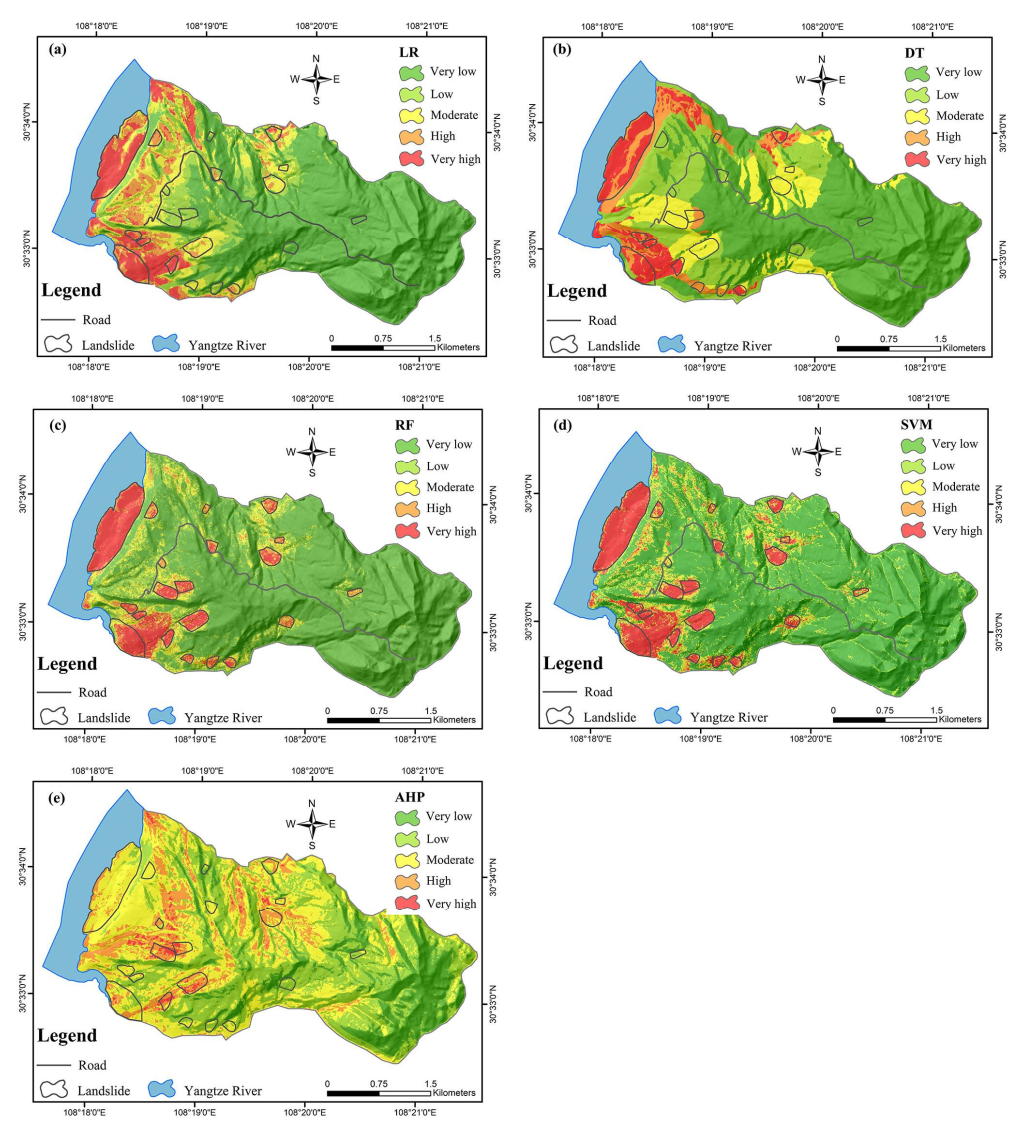
The landslide susceptibility index obtained from used models was divided into five levels according to the proportion: very high (10%), high (20%), moderate (20%), low (20%), and very low (30%). The susceptibility maps are shown in Figure 8.

5.1.3. Accuracy Comparison

After modelling, we used the ROC curve to compare the accuracy of these five models. As shown in Figure 9, the AUC of the RF model was the highest at 0.922; the others were 0.916 (SVM), 0.873 (DT), 0. 805 (LR) and 0. 722 (AHP). Therefore, based on the ROC curve, the RF model presents the best generalisation and accuracy in the regional LSM. In the following, “the original landslide susceptibility map” refers to the map produced by the RF model.

5.2. Landslide Susceptibility Modelling of G69

The AHP model was used to map the landslide susceptibility of G69 without landslide inventory. When using the AHP model for LSM, its decisions are taken using weights through pairwise relative comparisons. The final weights and quantitative values of all indicators are shown in Table 6.
Then, the weighted summation formula was used to calculate the landslide susceptibility index. It is given in Equation (3).
I = i , j = 1 m , n ω i x j ,
where n is the number of landslide causal factors, m is the categories number of each factor, ω i is the weight of the ith factor, and xj is the normalised values of the jth category of the factor.
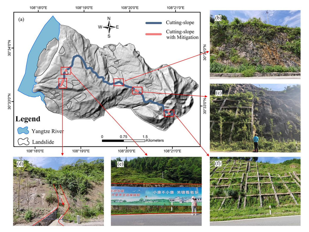
Subsequently, the landslide susceptibility index was divided into five grades: very high (10%), high (20%), moderate (20%), low (20%), and very low (30%). In the construction of G69, many treatment projects such as retaining structures or soil-improvement techniques have been applied, which can greatly reduce landslide hazards (Figure 10).
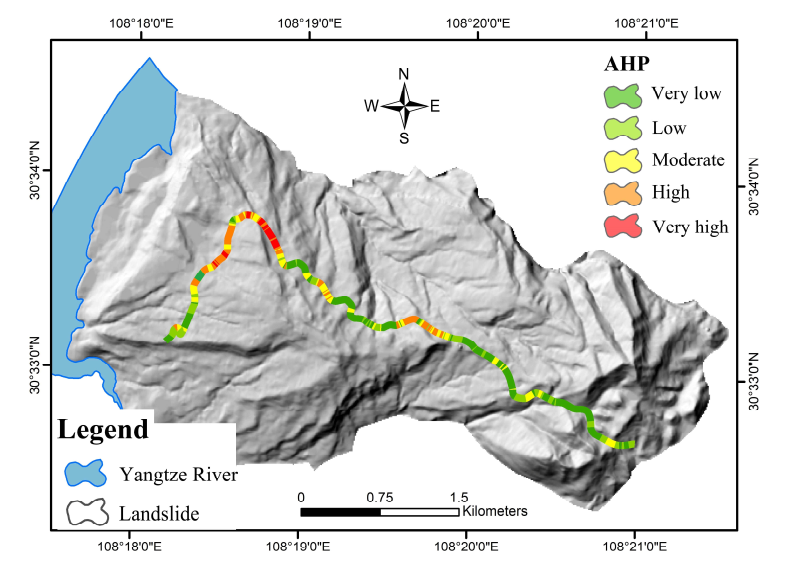
Finally, the method of downgrading to a very low susceptibility level if there is a treatment project was used to revise the landslide susceptibility of G69. The susceptibility maps of G69 are shown in Figure 11.

5.3. Fusion of Landslide Susceptibility Maps

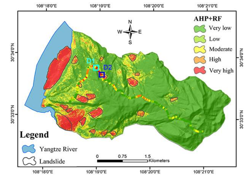
The final landslide susceptibility map was produced by combining the original landslide susceptibility map and the landslide susceptibility map of G69. The original landslide susceptibility map produced by the RF model shows the best accuracy, which was applied for the combination. During the fusion, we followed the principle of taking the maximum susceptibility value. The formula is shown in Equation (4).
I = I o v e r a l l   r e g i o n        I r o a d   r e g i o n < I o v e r a l l   r e g i o n   I r o a d   r e g i o n        I o v e r a l l   r e g i o n < I r o a d   r e g i o n   ,
where I is the final susceptibility index, Ioverall region is the original susceptibility index of the overall region, and Iroad area is the susceptibility index of the road area. After calculating by raster calculator in ArcGIS 10.6, the final landslide susceptibility map was produced (Figure 12).

6. Discussion

6.1. Landslide Distribution Partten

Landslide patterns usually show a great distinction in different areas due to the variation of the environment and materials involved; hence, the susceptibility models often perform variously [37]. In the study area of Wanzhou country, we explored the performance of four data-driven models (LR, DT, SVM, RF) and compared them with the AHP model. The results show that the RF model performed the best in LSM than SVM, DT, LR, and AHP (Figure 9). Similar to many studies [19,28,29], the RF model can be considered an effective tool in LSM because of its fast-modelling speed, adequate robustness, and accurate performance. In the case study, four regional landslide susceptibility maps show that most of the areas along the Yangtze River are in the high-susceptibility class (Figure 8). The reason for this is that the impoundment of reservoir water raised the susceptibility of the bank areas. Furthermore, the low-susceptibility class pixels are mainly located in the middle- and high-altitude areas. These areas are covered by limestone and quartz sandstone lithology, which do not easily cause landslide hazards. Hence, the evaluation results are more in line with reality. However, the G69 areas are classified as low susceptibility from the obtained maps, which is not consistent with the results of the field investigation.
The factor importance analysis by the RF model indicates that bedding structure, aspect, and lithology contribute the most to the LSM (Figure 7). Due to frequent disturbance at the foot, including lateral erosion and excavation, dip slopes are more prone to instability [45]. It considerably improves the factor importance of aspect. To understand laws governing landslides and underlying geomorphological process, the information values of each factor’s classes were calculated by Equation (2). In different bedding structures, the IV of dip slope (BS2) was the largest 0.988 (Table 1), having a promoting effect on the development of a landslide. Alternatively, the anaclinal slope (BS7) has the least promoting effect with the IV of −2.355. The above results are in good accordance with the investigation results, as landslide activity is clearly related to the shear strength parameters of the hillslope materials and slope structures. The failure of the dip slope is generally along the structural plane or weak intercalation, whereas the failure of the anaclinal slope is generally controlled by rock joints [46,47]. In a similar geological environment, the shear strength of the material in the dip slope, in general, is weaker than the anaclinal slope, which is more prone to landslide deformation.

6.2. Comparison of the Final Map and the Original Map

This paper explores a novel procedure coupling data and a heuristic model to LSM with limited landslide inventory. To determine whether there are statistically differences between the final map and the original map, the number of grids at each susceptibility level and their proportions are listed in Table 7. The results show that the proportion of the very-high-susceptibility class has increased by 2.4%, while the proportions of the low-, moderate-, and high-susceptibility class have decreased by 2.24%, 0.25%, and 0.14%, respectively. Therefore, this study effectively corrects the susceptibility class of the G69 area, which was underestimated due to the lack of landslide inventory in the map only obtained by the data-driven model.
A field investigation was also conducted for comparing and verifying the original and final maps. During the period from July to August 2020, two new landslides (D1 and D2) occurred along the road G69 (Figure 13). As can be seen in the final landslide susceptibility map (Figure 13), these two landslides are located in the high- and extremely-high-susceptibility levels, respectively, while in the original map produced by only the RF model, these two landslides are located in the low- and very-low-susceptibility levels (Figure 13). In view of the comparison results, we argue that a more accurate landslide susceptibility map can be obtained by modifying the AHP model. Hence, we recommend using the region-road-fusion process for LSM to overcome the limited landslides and obtain a more detailed susceptibility map, rather than focusing on creating new models or hybrid models.
In field work, we found that the impact of reservoirs water fluctuation on landslides is gradually weakening, which is in line with research by Zhang et al. [48]. At the same time, landslides induced by anthropogenic actions frequently occur in places where residents are concentrated and significantly impact people’s life, health, and economic development. Hence, in order to reduce the losses caused by landslides, we should pay more attention to the probability of landslide occurrence in places where residents are concentrated, especially in accurately calculating the landslide susceptibility after road construction, landslide engineering mitigation, and land-use changes.

7. Conclusions

In this research, a novel method has been proposed for landslide susceptibility mapping, suitable for areas with heterogeneous completeness of landslides inventories. In particular, the method combines data-driven and knowledge-driven approaches. The proposed approach has been applied to an area receiving road construction in Wanzhou, China. The data-driven approach has been applied to derive a first regional landslide susceptibility map valid for the whole area, except in the nearby of the road. The knowledge-driven method has then been used to derive susceptibility in the vicinity of the road (lower completeness of the landslide inventory). The following conclusions can be drawn from the present analysis: (a) For the regional map, among the four tested data-driven models (RF, SVM, DT, LR), RF has the greatest accuracy. (b) Due to the lack of landslide samples, the landslide susceptibility class in G69 areas cannot be accurately produced by the data-driven models. A knowledge-driven approach (AHP) is more suitable to obtain landslide susceptibility in the vicinity of road G69. (c) In the final map, combining the original regional map (RF) with the AHP map, the proportion of the very-high-susceptibility class has increased by 2.4%. Two new landslides developed along G69 are the robust evidence to prove it. Hence, the proposed fusion process for LSM has been successful in overcoming the issue of incomplete landslide inventories along human-modified areas within a broader region.

Author Contributions

Conceptualisation, L.Y. and C.Z.; software, L.Y.; investigation, L.Y. and C.Z.; writing—original draft preparation, L.Y. and D.J.P.; writing—review and editing, C.Z., Y.C. and Y.W.; supervision, C.Z., Y.C. and Y.W.; funding acquisition, Y.W. All authors have read and agreed to the published version of the manuscript.

Funding

This research was funded by the National Natural Science Foundation of China, grant numbers 41907253 and 41702330.

Institutional Review Board Statement

Not applicable.

Informed Consent Statement

Not applicable.

Data Availability Statement

Data sharing not applicable.

Conflicts of Interest

The authors declare no conflict of interest.

References

  1. Reichenbach, P.; Rossi, M.; Malamud, B.; Mihir, M.; Guzzetti, F. A review of statistically-based landslide susceptibility models. Earth Sci. Rev. 2018, 180, 60–91. [Google Scholar] [CrossRef]
  2. Ma, S.Y.; Xu, C.; Xu, X.W.; He, X.L.; Qian, H.T.; Jiao, Q.S.; Gao, W.; Yang, H.N.; Cui, Y.L.; Zhang, P.F.; et al. Characteristics and causes of the landslide on July 23, 2019 in Shuicheng, Guizhou Province, China. Landslides 2020, 17, 1441–1452. [Google Scholar] [CrossRef]
  3. Gao, Y.; Yin, Y.; Li, B.; Feng, Z.; He, K. Characteristics and Numerical Runout Modeling Analysis of the Jiweishan Landslide, Chongqing, China. Environ. Eng. Geosci. 2018, 24, 413–423. [Google Scholar]
  4. Weidinger, J.T. Predesign, failure and displacement mechanisms of large rockslides in the Annapurna Himalayas, Nepal. Eng. Geol. 2006, 83, 201–216. [Google Scholar] [CrossRef]
  5. Khanna, K.; Martha, T.R.; Roy, P.; Kumar, K.V. Effect of time and space partitioning strategies of samples on regional landslide susceptibility modelling. Landslides 2021, 18, 2281–2294. [Google Scholar] [CrossRef]
  6. Corominas, J.; Westen, C.V.; Frattini, P.; Cascini, L.; Malet, J.P.; Fotopoulou, S.; Catani, F.; Van Den Eeckhaut, M.; Mavrouli, O.; Agliardi, F.; et al. Recommendations for the quantitative analysis of landslide risk. Bulletin of engineering geology and the environment. Bull. Eng. Geol. Environ. 2014, 73, 209–263. [Google Scholar]
  7. Castellanos, A.; Enrique, A.; Van Westen, C.J. Qualitative landslide susceptibility assessment by multicriteria analysis: A case study from San Antonio del Sur, Guantánamo, Cuba. Geomorphology 2008, 94, 453–466. [Google Scholar] [CrossRef] [Green Version]
  8. Ma, J.R.; Zhang, T.H.; Guan, X.D.; Hu, X.M.; Duan, A.M.; Liu, J.C. The dominant role of snow/ice albedo feedback strengthened by black carbon in the enhanced warming over the Himalayas. J. Clim. 2019, 32, 5883–5899. [Google Scholar] [CrossRef]
  9. Mirus, B.B.; Jones, E.S.; Baum, R.L.; Godt, J.W.; Slaughter, S.; Crawford, M.M.; Lancaster, J.; Stanley, T.; Kirschbaum, D.B.; Burns, W.J.; et al. Landslides across the USA: Occurrence, susceptibility, and data limitations. Landslides 2020, 17, 2271–2285. [Google Scholar] [CrossRef]
  10. Al-Najjar, H.A.H.; Kalantar, B.; Pradhan, B.; Saeidi, V. Conditioning factors determination for mapping and prediction of landslide susceptibility using machine learning algorithms. In Proceedings of the Earth Resources and Environmental Remote Sensin, Strasbourg, France, 10–12 September 2019. [Google Scholar]
  11. Sharma, L.; Patel, N.; Ghose, M.; Debnath, P. Development and application of Shannon’s entropy integrated information value model for landslide susceptibility assessment and zonation in Sikkim Himalayas in India. Nat. Hazards 2015, 75, 1555–1576. [Google Scholar] [CrossRef]
  12. Ayalew, L.; Yamagishi, H. The application of GIS-based logistic regression for landslide susceptibility mapping in the Kakuda-Yahiko Mountains, Central Japan. Geomorphology 2005, 65, 15–31. [Google Scholar] [CrossRef]
  13. Pradhan, B.; Lee, S. Landslide susceptibility assessment and factor effect analysis: Backpropagation artificial neural networks and their comparison with frequency ratio and bivariate logistic regression modelling. Environ. Modell. Softw. 2010, 25, 747–759. [Google Scholar] [CrossRef]
  14. Zhou, C.; Cao, Y.; Yin, K.; Ahmed, B.; Li, Y.; Catani, F.; Pourghasemi, H. Landslide susceptibility modeling applying machine learning methods: Acase study from Longju in the Three Gorges Reservoir area, China. Comput. Geosci. 2018, 112, 23–27. [Google Scholar] [CrossRef] [Green Version]
  15. Wu, X.; Fu, R.; Niu, R. Landslide susceptibility assessment using object mapping units, decision tree, and support vector machine models in the three gorges of China. Environ. Earth Sci. 2014, 71, 4725–4738. [Google Scholar] [CrossRef]
  16. Wu, Y.; Ke, Y.; Chen, Z.; Liang, S.; Hong, H. Application of Alternating Decision Tree with AdaBoost and Bagging ensembles for landslide susceptibility mapping. Catena 2020, 187, 104396. [Google Scholar] [CrossRef]
  17. San, B.T. An evaluation of SVM using polygon-based random sampling in landslide susceptibility mapping: The Candir catchment area (western Antalya, Turkey). Int. J. Appl. Earth Obs. Geoinf. 2014, 26, 399–412. [Google Scholar] [CrossRef]
  18. Lee, S.; Hong, S.M.; Jung, H.S. A Support Vector Machine for Landslide Susceptibility Mapping in Gangwon Province, Korea. Sustainability 2017, 9, 48. [Google Scholar] [CrossRef] [Green Version]
  19. Sun, D.; Xu, J.; Wen, H.; Wang, Y. An Optimized Random Forest Model and Its Generalization Ability in Landslide Susceptibility Mapping: Application in Two Areas of Three Gorges Reservoir, China. J. Earth Sci. 2020, 31, 1068–1086. [Google Scholar] [CrossRef]
  20. Bui, D.T.; Tran, A.T.; Klempe, H.; Pradhan, B.; Revhaug, I. Spatial prediction models for shallow landslide hazards: A comparative assessment of the efficacy of support vector machines, artificial neural networks, kernel logistic regression, and logistic model tree. Landslides 2016, 13, 361–378. [Google Scholar]
  21. Scaioni, M.; Longoni, L.; Melillo, V.; Papini, M. Remote Sensing for Landslide Investigations: An Overview of Recent Achievements and Perspectives. Remote Sens. 2014, 6, 9600–9652. [Google Scholar] [CrossRef] [Green Version]
  22. Zhou, C.; Cao, Y.; Yin, K.; Wang, Y.; Shi, X.; Catani, F.; Ahmed, B. Landslide characterization applying Sentinel-1 images and InSAR technique: The Muyubao landslide in the three gorges reservoir area, China. Remote Sens. 2020, 12, 3385. [Google Scholar] [CrossRef]
  23. Song, Y.H. Failure Models and Instability of Slopes with Soft and Hard Interbedded Laminated Structure in Southwest China; Chengdu University of Technology: Chengdu, China, 2011. [Google Scholar]
  24. Pellicani, R.; Argentiero, I.; Spilotro, G. GIS-based predictive models for regional-scale landslide susceptibility assessment and risk mapping along road corridors. Geomat. Nat. Hazards 2017, 8, 1012–1033. [Google Scholar] [CrossRef] [Green Version]
  25. Acharya, T.; Lee, D. Landslide Susceptibility Mapping using Relative Frequency and Predictor Rate along Araniko Highway. J. Civ. Eng. 2019, 23, 763–776. [Google Scholar] [CrossRef]
  26. Keller, S.; Atzl, A. Assessment of forest road conditions in terms of landslide susceptibility: A case study in Yigilca Forest Directorate (Turkey). Turk. J. Agric. For. 2014, 38, 281–290. [Google Scholar]
  27. Wang, J.J.; Xiao, L.L.; Zhang, J.; Zhu, Y.B. Deformation characteristics and failure mechanisms of a rainfall-induced complex landslide in Wanzhou County, Three Gorges Reservoir, China. Landslides 2019, 17, 419–431. [Google Scholar] [CrossRef]
  28. Nhu, V.H.; Shirzadi, A.; Shahabi, H.; Chen, W.; Lee, S. Shallow Landslide Susceptibility Mapping by Random Forest Base Classifier and Its Ensembles in a Semi-Arid Region of Iran. Forests 2020, 11, 421. [Google Scholar] [CrossRef] [Green Version]
  29. Zheng, H. Improved landslide assessment using support vector machine with bagging, boosting, and stacking ensemble machine learning framework in a mountainous watershed, Japan. Landslides 2020, 17, 641–658. [Google Scholar]
  30. Marjanovic, M.; Kovacevic, M.; Bajat, B.; Vozenilek, V. Landslide susceptibility assessment using SVM machine learning algorithm. Eng. Geol. 2011, 123, 225–234. [Google Scholar] [CrossRef]
  31. Du, J.; Glade, T.; Woldai, T.; Chai, B.; Zeng, B. Landslide susceptibility assessment based on an incomplete landslide inventory in the Jilong Valley, Tibet, Chinese Himalayas. Eng. Geol. 2020, 270, 105572. [Google Scholar] [CrossRef]
  32. Huang, D.; Luo, S.; Zhong, Z.; Gu, D.; Song, Y.; Tomas, R. Analysis and modeling of the combined effects of hydrological factors on a reservoir bank slope in the Three Gorges Reservoir area, China. Eng. Geol. 2020, 279, 105858. [Google Scholar] [CrossRef]
  33. Li, Y.; Utili, S.; Milledge, D.; Chen, L.; Yin, K. Chasing a complete understanding of the failure mechanisms and potential hazards of the slow-moving Liangshuijing landslide. Eng. Geol. 2020, 28, 10597. [Google Scholar] [CrossRef]
  34. He, K.; Li, X.; Yan, X.; Guo, D. The landslides in the Three Gorges Reservoir Region, China and the effects of water storage and rain on their stability. Environ. Geol. 2008, 55, 55–63. [Google Scholar]
  35. Moore, I.D.; Grayson, R.B.; Ladson, A.R. Digital terrain modelling: A review of hydrological, geomorphological, and biological applications. Hydrol. Process. 1991, 5, 3–30. [Google Scholar] [CrossRef]
  36. Beven, K.J.; Moore, I.D. Terrain Analysis and Distributed Modelling in Hydrology; Wiley Sons: London, UK, 1993. [Google Scholar]
  37. Yu, L.; Cao, Y.; Zhou, C.; Wang, Y.; Huo, Z. Landslide Susceptibility Mapping Combining Information Gain Ratio and Support Vector Machines: A Case Study from Wushan Segment in the Three Gorges Reservoir Area, China. Appl. Sci. 2019, 9, 4756. [Google Scholar] [CrossRef] [Green Version]
  38. Hencher, S. Preferential flow paths through soil and rock and their association with landslides. Hydrol. Process. 2010, 24, 1610–1630. [Google Scholar] [CrossRef]
  39. Peng, L.; Niu, R.; Bo, H.; Wu, X.; Zhao, Y.; Ye, R. Landslide susceptibility mapping based on rough set theory and support vector machines: A case of the Three Gorges area, China. Geomorphology 2014, 204, 287–301. [Google Scholar] [CrossRef]
  40. Bhandary, N.P.; Dahal, R.K.; Timilsina, M.; Yatabe, R. Rainfall event-based landslide susceptibility zonation mapping. Nat. Hazards. 2020, 69, 365–388. [Google Scholar] [CrossRef]
  41. Li, S.; Xu, Q.; Tang, M.; Iqbal, J.; Liu, J.; Zhu, X.; Liu, F.; Zhu, D. Characterizing the spatial distribution and fundamental controls of landslides in the three gorges reservoir area, China. Bull. Eng. Geol. Environ. 2019, 78, 4275–4290. [Google Scholar] [CrossRef]
  42. Bi, R.; Schleier, M.; Rohn, J.; Ehret, D.; Xiang, W. Landslide susceptibility analysis based on ArcGIS and Artificial Neural Network for a large catchment in Three Gorges region, China. Environ. Earth Sci. 2014, 72, 1925–1938. [Google Scholar] [CrossRef]
  43. Maldonado, S.; López, J. Dealing with high-dimensional class-imbalanced datasets: Embedded feature selection for svm classification. Appl. Soft. Comput. 2018, 67, 94–105. [Google Scholar] [CrossRef]
  44. Liu, L.; Yang, C.; Wang, X. Landslide susceptibility assessment using feature selection-based machine learning models. Geomech. Eng. 2021, 25, 1–16. [Google Scholar]
  45. Gong, W.; Wang, P.; Chen, L. Analysis of sensitivity factors to stability of bedding rock cutting slope. Rock Soil Mech. 2007, 28, 812–816. [Google Scholar]
  46. Chai, B.; Yin, K.L. Influence of intersection angle between trend of slope and strata on stability of bedding slope. Chin. J. Rock Mech. Eng. 2009, 28, 624–628. [Google Scholar]
  47. Cheng, Q.; Zhou, P.D.; Feng, Z.J. Research on shear creep property of typical weak intercalation in red bed soft rock. Chin. J. Rock Mech. Eng. 2009, 28, 3176. [Google Scholar]
  48. Li, S.L. Study on the Reactivation Characteristic and Deformation Self-Adaptive of Landslide in the Three Gorges Reservoir Area; Chengdu University of Technology: Chengdu, China, 2020. [Google Scholar]
Figure 1. (a) The map of China; (b) The map of Wanzhou; (c) Landslide locations of the study area; (d) Geological section of 1–1′.
Remotesensing 14 00774 g001
Figure 2. (a) Aerial view of the Jinjinzi landslide; (b) The active deformation zone of Jinjinzi landslide; (c) Aerial view of the Tongzilin landslide; (d) Observed tensile cracks on the right boundary of Tongzilin landslide.
Remotesensing 14 00774 g002
Figure 3. The flow chart of the proposed framework.
Remotesensing 14 00774 g003
Figure 4. Thematic maps of landslide causal factors: (a) altitude, (b) slope, (c) aspect, (d) curvature, (e) plan curvature, (f) profile curvature, (g) TRI, (h) TWI, (i) distance to rivers, (j) distance to roads, (k) lithology, (l) bedding structure.
Remotesensing 14 00774 g004aRemotesensing 14 00774 g004b
Figure 5. Landslide causal factors of the road affected area: (a) slope, (b) bedding structure, (c) rock mass structure, (d) rock association, (e) cutting height, (f) overburden thickness.
Remotesensing 14 00774 g005
Figure 6. Classification of rock association (RA1:Huge-thick hard rock intercalated with soft layer. RA2: Medium-thick hard rock with soft rock. RA3: Medium-thick hard rock with thin hard rock. RA4: Upper soft rock and lower hard rock. RA5: Upper hard rock and lower soft rock. RA6: Interbedded soft and hard rocks. RA7: Soft rock as main hard rock. RA8 soft rock. RA9 hard rock).
Remotesensing 14 00774 g006
Figure 7. Causal factors importance plot.
Remotesensing 14 00774 g007
Figure 8. The landslide susceptibility maps produced by (a) LR, (b) DT, (c) RF, (d) SVM, and (e) AHP models.
Remotesensing 14 00774 g008
Figure 9. ROC curves and AUC analysis for the AHP, DT, SVM, RF, and LR models using the validating data.
Remotesensing 14 00774 g009
Figure 10. (a) The map of G69; (b) Cutting-slope without mitigation; (c) Cutting-slope with soil improvement techniques; (d) Cutting-slope with drainage techniques; (e) Cutting-slope with retaining wall; (f) Cutting-slope with retaining structure.
Remotesensing 14 00774 g010
Figure 11. The G69 landslide susceptibility map based on AHP model.
Remotesensing 14 00774 g011
Figure 12. The final landslide susceptibility map.
Remotesensing 14 00774 g012
Figure 13. The comparison between the landslide susceptibility map based on only the RF model and the one revised from the AHP model. (a) Two susceptibility maps and photo of the D1 landslide. (b) Two susceptibility maps and photo of the D2 landslide. (The locations of two new landslides are shown in Figure 12.)
Remotesensing 14 00774 g013
Table 1. Spatial relationships between landslide causal factors and landslides using IV model.
FactorsClassPLPTDPLTLPDTDIVNormalised Class
Altitude (m)<250742724,1370.64 0.20 1.150.99
250~425390744,8560.33 0.37 −0.110.65
425~50019422,9320.02 0.19 −2.440.01
500~55016497730.01 0.08 −1.76 0.19
>550018,3440.00 0.15 0.01
Slope (°)<6199278740.17 0.07 0.950.99
6~15570638,6480.49 0.32 0.420.83
15~24296138,4010.25 0.32 −0.230.63
24~3693824,6420.08 0.21 −0.940.41
36~489591450.01 0.08 −2.240.01
48~69013320.00 0.01 0.01
Aspect (°)0~4595117,2780.08 0.14 −0.570.67
45~9021298600.02 0.08 −1.510.39
90~1352237130.00 0.03 −2.800.01
135~18033183210.03 0.07 −0.89 0.57
180~225149517,4950.13 0.15 −0.130.8
225~270214518,0640.18 0.15 0.190.9
270~315479328,8710.41 0.24 0.530.99
315~360174316,4400.15 0.14 0.080.86
Curvature−15 to −12510729730.01 0.02 −1.000.01
0 to −15202924,4610.170.20−0.160.71
0~5829971,0770.710.590.180.99
5~66125721,5310.11 0.18−0.510.41
Plan curvature−58 to −350350.00 0.00 0.01
−35 to −526258810.02 0.05 −0.780.01
−5 to 0615955,8620.53 0.47 0.120.99
0~25527158,2490.45 0.49 −0.070.78
25~300150.00 0.00 0.01
Profile curvature−53 to −400160.00 0.00 0.01
−2 to −40226132,0640.19 0.27 −0.320.07
−2 to 5858875,4010.73 0.63 0.150.99
5~3084312,4230.07 0.10 −0.360.01
30~7601380.00 0.00 0.01
Topographic roughness index 0~1.110,74886,5590.920.720.240.99
1.1~1.275119,3030.060.16−0.920.67
1.2~1.317080410.010.07−1.530.49
>1.32361390.000.05−3.260.01
Topographic wetness index −3.4 to −271413,1590.06 0.11 −0.580.01
−2 to 1130879890.11 0.07 0.520.99
1~5376053,2130.32 0.44 −0.320.24
5~15591045,6610.51 0.38 0.280.78
15~170200.00 0.00 0.01
Distance to rivers (m)0~100111916,9680.10 0.14 −0.390.29
100~250554244,6020.47 0.37 0.240.99
250~500450048,0410.38 0.40 −0.040.68
>50053110,4310.05 0.09 −0.650.01
Distance to roads (m)0~100391938,8650.34 0.32 0.030.95
100~250569054,0830.49 0.45 0.080.99
250~450185921,8210.16 0.18 −0.130.76
>45022452730.02 0.04 −0.830.01
Lithology L1066660.00 0.06 0.01
L2272227,9150.23 0.23 0.010.46
L3602050,5560.51 0.42 0.200.60
L475015,1730.06 0.13 −0.670.01
L554510,3650.05 0.09 −0.610.04
L641319080.04 0.02 0.800.99
L7124275000.11 0.06 0.530.82
Bedding structure BS170568520.06 0.06 0.060.72
BS2511119,5350.44 0.16 0.990.99
BS3188324,2310.16 0.20 −0.230.64
BS4174724,3660.15 0.20 −0.310.61
BS5193029,4080.17 0.24 −0.390.58
BS626810,4570.02 0.09 −1.330.30
BS74851930.00 0.04 −2.350.01
Note: PL = pixels in landslide, PTD = pixels in total domain, PLTL = proportion of landslide in total landslide, PDTD = proportion of domain in total domain.
Table 2. Multicollinearity of the causal factors.
FactorOriginal FactorNew Factor
TolerancesVIFTolerancesVIF
Altitude0.7971.2540.6291.590
Slope0.2344.2710.6321.583
Aspect0.9091.1000.8241.214
Plan curvature0.8731.1450.7311.369
Profile curvature0.6431.5550.6471.544
TRI0.2524.969//
TWI0.8071.2400.8991.112
Lithology0.9181.0900.9511.051
Bedding structure0.7481.3370.6391.565
Distance to rivers0.9751.0260.8441.185
Distance to road0.9441.0590.8791.138
Table 3. The prediction accuracy after eliminating factors.
ModelEliminating Less Important FactorsAccuracy
Model 1Without eliminating any factor0.824
Model 2Profile curvature0.914
Model 3Plan curvature0.917
Model 4Profile curvature, plan curvature0.907
Model 5Curvature0.904
Model 6TWI, profile curvature, plan curvature, curvature0.901
Model 7TWI, slope, profile curvature, plan curvature, curvature0.901
Table 4. Description of 10 causal factors and grade scores of variables in AHP model.
FactorsWeightCategories (Normalised Values)
Altitude (m)0.108<250(0.35), 250~425(0.3), 425~500(0.17), 500~550(0.15), >550(0.03)
Slope (°)0.161<6(0.24), 6~15(0.32), 15~24(0.21), 24~36(0.1),
36~48(0.05), 48~69(0.05)
Aspect (°)0.0960~45(0.07), 45~90(0.03), 90~135(0.07), 135~180(0.11), 180~225(0.11), 225~270(0.17), 270~315(0.27), 315~360(0.17)
Curvature0.021−125 to −15(0.21), −15 to 0(0.27), 0~5(0.31), 5~66(0.21)
Profile curvature0.014−53 to −40(0.11), −40 to −2(0.17), −2 to 5(0.4),
5~30(0.21), 30~76(0.11)
TWI0.021−3.4 to −2(0.07), −2 to 1(0.37), 1~5(0.25), 5~15(0.2), 15~17(0.11)
Distance to rivers (m)0.1560~100(0.45), 100~250(0.31), 250~500(0.15), >500(0.09)
Distance to roads (m)0.0410~100(0.35), 100~250(0.25), 250~450(0.22), >450(0.18)
Lithology0.161L1(0.05), L2(0.11), L3(0.11), L4(0.05),
L5(0.11), L6(0.37), L7(0.3)
Bedding structure0.221BS1(0.2), BS2(0.32), BS3(0.15), BS4(0.11),
BS5(0.07), BS6(0.11), BS7(0.05)
Table 5. The parameters of four models.
ModelParametersNotes
LRC = 0.3C is the reciprocal of regularisation strength.
DTmax_depth = 4Max_depth is the maximum depth of the tree.
RFn_estimators = 73, max_depth = 30n_estimators is the number of trees in random forests, max_depth is the maximum depth of the tree.
SVMC = 5, gamma = 0.45C is the penalty term coefficient of the relaxation coefficient, and gamma is the coefficient of the kernel function.
Table 6. Causal factors and grade scores of variables in AHP model.
FactorsWeightCategoriesNormalised ValuesFactorsWeightCategoriesNormalised Values
Slope/(°)0.1194<100.130Overburden thickness/(m)0.081<0.50.123
10~200.1930.5~10.198
20~300.2521~1.50.316
>300.425>1.50.363
Rock association0.2287RA10.155Rock mass structure0.148Massive structure0.068
RA20.072Interlayer structure0.149
RA30.145Layer structure0.115
RA40.07Fragmented structure0.163
RA50.101Thin layer structure0.145
RA60.103Blocky structure0.079
RA70.075Scattered structure0.281
RA80.087Bedding structure0.2829BS10.086
RA90.053BS20.110
Cutting height/(m)0.1400.061BS30.119
0~50.104BS40.131
5~100.165BS50.139
10~200.251BS60.179
>200.418BS70.234
Table 7. Statistical analysis of the proportion of each susceptibility class.
Susceptibility LevelOriginal Map (RF)Final Map (AHP + RF)Variation
PixelsProportionPixelsProportion
Very low82, 42168.66%82,73868.92%+0.23%
Low13, 58911.32%10,9509.12%−2.24%
Moderate8, 4157.01%82516.87%−0.14%
High5, 2104.34%48154.01%−0.25%
Very high10, 4088.67%13,28911.07%+2.4%
Publisher’s Note: MDPI stays neutral with regard to jurisdictional claims in published maps and institutional affiliations.