
Enhanced TabNet: Attentive Interpretable Tabular Learning for Hyperspectral Image Classification


Abstract
:1. Introduction
- It introduces TabNet for HSI classification and improves classification performance by applying unsupervised pretraining in uTabNet;
- It develops TabNets and uTabNets after including spatial information in the attentive transformer;
- It includes SP in sTabNet as a feature extraction to further improve the classification performance of SP versions of TabNet, i.e., suTabNet, sTabNets, and suTabNets.
2. Related Work
2.1. Tree Based Learning
2.2. Attentive Interpretable Tabular Learning (TabNet)
3. Proposed Method
3.1. TabNet for Hyperspectral Image Classification
- (1)
- The “split” module separates the output of the initial feature transformer to obtain features in Step 1 when i = 1;
- (2)
- If we disregard the spatial information in the attentive transformer of TabNets shown in Figure 4 below, it becomes the attentive transformer for TabNet. It uses a trainable function , consisting of a fully connected (FC) and batch normalization (BN) layer to generate features with high dimensions;
- (3)
- In each step, interpretable information is provided by masks for selecting features, and global interpretability can be attained by aggregating the masks from different decision steps. This process can enhance the discriminative ability in the spectral domain by implementing local and global interpretability for HSI feature selection.
- (4)
- The sparsity regularization term can be used in the form of entropy [57] for controlling the sparsity of selected features.
- (5)
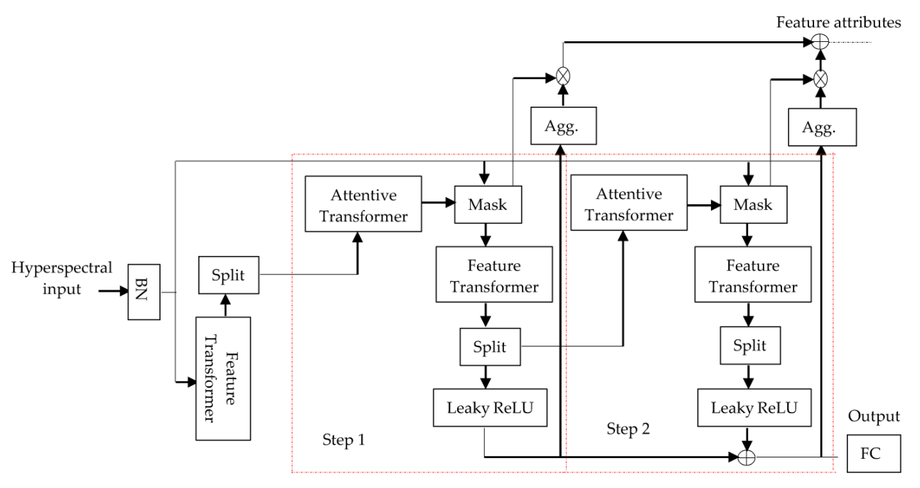
- A sequential multi-step decision process with is used in TabNet’s encoding. The processed information from step is passed to the step to decide which features to use. The outputs are obtained by aggregating the processed feature representation in the overall decision function as shown by feature attributes in Figure 1.
- (1)
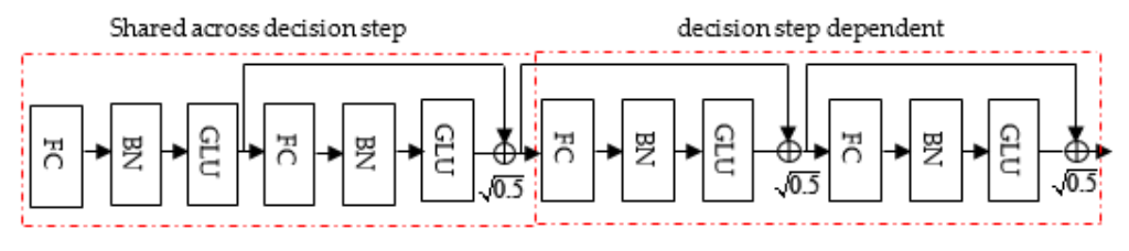
- The feature transformer in Figure 2 is used to process the filtered features, which can be used in the decision step output and information for subsequent steps:
- (2)
- For efficient learning with high capacity, the feature transformer is comprised of layers that are shared across decision steps such that the same features can be input for different decision steps, and decision step-dependent layers in which features in the current decision step depend upon the output from the previous decision step;
- (3)
- In Figure 2, it can be observed that the feature transformer consists of the concatenation of two shared layers and two decision step-dependent layers, in which each fully connected (FC) layer is followed by batch normalization (BN) and a gated linear unit (GLU) [58]. Normalization with is also used for ensuring stabilized learning throughout the network [59];
- (4)
- All BN operations, except applied at input features, are implemented in ghost BN [60] by selecting only part of samples rather than using an entire batch at one time to reduce the cost of computation. This improves performance by using the virtual or small batch size and momentum instead of using the entire batch. Moreover, decision tree-like aggregation is implemented by constructing overall decision embedding as:where represents the number of decision steps;
- (5)
- The linear mapping is applied for output mapping and softmax is employed during training for discrete outputs.
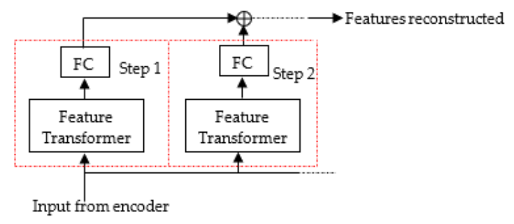
3.2. TabNet with Unsupervised Pretraining
3.3. TabNet with Spatial Attention (TabNets)
- (1)
- The first BN generates a 6250 × 1 vector;
- (2)
- It is converted by the first feature transformer layer before Step 1 into a feature vector of size ;
- (3)
- The Split layer divides it into two parts and provides a feature of size for the attentive transformer;
- (4)
- The Attentive transformer layer generates output masks for the 6250 × 1 feature;
- (5)
- The Mask layer in Step 1 generates the multiplicative output to the feature transformer layer with the 6250 × 1 feature;
- (6)
- The feature transformer generates the feature of size , which is separated into two parts: in LeakyReLu and for the attentive transformer in Step 1;
- (7)
- The output of each decision step is then concatenated in the TabNets encoder and converted to a feature map with 16 classes by the FC layer.
- (1)
- The output of from Equation (1) is reshaped to as input to the first 2D convolution layer. For a kernel size of and stride = 3, the first 2D convolution layer provides a output;
- (2)
- The second convolution layer generates an output of size with a kernel size of and stride = 1;
- (3)
- The third convolutional layer generates an output shape of with a kernel size of and stride = 1;
- (4)
- The flatten layer provides an output of size 1024 × 1;
- (5)
- Finally, the FC layer generates an output of size 6250 × 1 that is provided as input to the prior scales for updating the abstract features generated by the FC and BN layers inside the attentive transformer.
3.4. Structure Profile on TabNet (sTabNet)
3.5. Structure Profile on Unsupervised Pretrained TabNet (suTabNet)
4. Experiments
4.1. Datasets
4.2. Experimental Setup
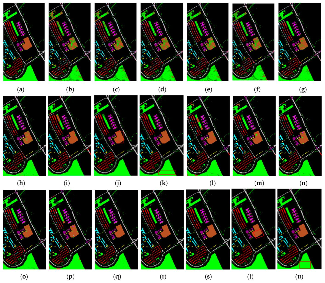
4.3. Result of Classification
5. Conclusions
Author Contributions
Funding
Acknowledgments
Conflicts of Interest
References
- Shah, C.; Du, Q. Collaborative and Low-Rank Graph for Discriminant Analysis of Hyperspectral Imagery. IEEE J. Sel. Top. Appl. Earth Obs. Remote Sens. 2021, 14, 5248–5259. [Google Scholar] [CrossRef]
- Shah, C.; Du, Q. Spatial-Aware Probabilistic Collaborative Representation for Hyperspectral Image Classification. In Proceedings of the Image and Signal Processing for Remote Sensing XXVI (Proc. Of SPIE), Edinburgh, UK, 21–25 September 2020. art no 115330Q. [Google Scholar] [CrossRef]
- Li, W.; Du, Q. Joint Within-Class Collaborative Representation for Hyperspectral Image Classification. IEEE J. Sel. Top. Appl. Earth Obs. Remote Sens. 2014, 7, 2200–2208. [Google Scholar] [CrossRef]
- Shah, C.; Du, Q. Modified Structure-Aware Collaborative Representation for Hyperspectral Image Classification. In Proceedings of the 2021 IEEE International Geoscience and Remote Sensing Symposium IGARSS, Brussels, Belgium, 11–16 July 2021. [Google Scholar] [CrossRef]
- Pan, L.; Li, H.-C.; Deng, Y.-J.; Zhang, F.; Chen, X.-D.; Du, Q. Hyperspectral Dimensionality Reduction by Tensor Sparse and Low-Rank Graph-Based Discriminant Analysis. Remote Sens. 2017, 9, 452. [Google Scholar] [CrossRef] [Green Version]
- Li, W.; Wang, Z.; Li, L.; Du, Q. Feature extraction for hyperspectral images using local contain profile. IEEE J. Sel. Top. Appl. Earth Obs. Remote Sens. 2019, 12, 5035–5046. [Google Scholar] [CrossRef]
- Hong, D.; Wu, X.; Ghamisi, P.; Chanussot, J.; Yokoya, N.; Zhu, X.X. Invariant attribute profiles: A spatial-frequency joint feature extractor for hyperspectral image classification. IEEE Trans. Geosci. Remote Sens. 2020, 58, 3791–3808. [Google Scholar] [CrossRef] [Green Version]
- Chang, C.-I. Hyperspectral Data Exploitation: Theory and Applications; Wiley: Hoboken, NJ, USA, 2007. [Google Scholar] [CrossRef]
- Chen, M.; Tang, Y.; Zou, X.; Huang, Z.; Zhou, H.; Chen, S. 3D global mapping of large-scale unstructured orchard integrating eye-in-hand stereo vision and SLAM. Comput. Electron. Agric. 2021, 187, 106237. [Google Scholar] [CrossRef]
- Wu, F.; Duan, J.; Chen, S.; Ye, Y.; Ai, P.; Yang, Z. Multi-Target Recognition of Bananas and Automatic Positioning for the Inflorescence Axis Cutting Point. Front. Plant Sci. 2021, 12, 705021. [Google Scholar] [CrossRef]
- Cao, X.; Yan, H.; Huang, Z. A Multi-Objective Particle Swarm Optimization for Trajectory Planning of Fruit Picking Manipulator. Agronomy 2021, 11, 2286. [Google Scholar] [CrossRef]
- Du, P.; Samat, A.; Waske, B.; Liu, S.; Li, Z. Random Forest and rotation forest for fully polarized SAR image classification using polarimetric and spatial features. ISPRS J. Photogramm. Remote Sens. 2015, 105, 38–53. [Google Scholar] [CrossRef]
- Samat, A.; Persello, C.; Liu, S.; Li, E.; Miao, Z.; Abuduwaili, J. Classification of VHR multispectral images using extratrees and maximally stable extremal region-guided morphological profile. IEEE J. Sel. Top. Appl. Earth Obs. Remote Sens. 2018, 11, 3179–3195. [Google Scholar] [CrossRef]
- Melgani, F.; Bruzzone, L. Classification of Hyperspectral Remote Sensing Images with Support Vector Machines. IEEE Trans. Geosci. Remote Sens. 2004, 42, 1778–1790. [Google Scholar] [CrossRef] [Green Version]
- Camps-Valls, G.; Gomez-Chova, L.; Munoz-Mari, J.; Vila-Frances, J.; Calpe-Maravilla, J. Composite Kernels for Hyperspectral Image Classification. IEEE Geosci. Remote Sens. Lett. 2006, 3, 93–97. [Google Scholar] [CrossRef]
- Li, J.; Bioucas-Dias, J.M.; Plaza, A. Spectral–Spatial Hyperspectral Image Segmentation Using Subspace Multinomial Logistic Regression and Markov Random Fields. IEEE Trans. Geosci. Remote Sens. 2012, 50, 809–823. [Google Scholar] [CrossRef]
- Hughes, G. On the Mean Accuracy of Statistical Pattern Recognizers. IEEE Trans. Inf. Theory 1968, 14, 55–63. [Google Scholar] [CrossRef] [Green Version]
- Fauvel, M.; Tarabalka, Y.; Benediktsson, J.A.; Chanussot, J.; Tilton, J.C. Advances in Spectral-Spatial Classification of Hyperspectral Images. Proc. IEEE 2013, 101, 652–675. [Google Scholar] [CrossRef] [Green Version]
- Cui, M.; Prasad, S. Class-Dependent Sparse Representation Classifier for Robust Hyperspectral Image Classification. IEEE Trans. Geosci. Remote Sens. 2015, 53, 2683–2695. [Google Scholar] [CrossRef]
- Wright, J.; Yang, A.Y.; Ganesh, A.; Sastry, S.S.; Yi, M. Robust Face Recognition via Sparse Representation. IEEE Trans. Pattern Anal. Mach. Intell. 2009, 31, 210–227. [Google Scholar] [CrossRef] [Green Version]
- Chen, Y.; Nasrabadi, N.M.; Tran, T.D. Hyperspectral Image Classification Using Dictionary-Based Sparse Representation. IEEE Trans. Geosci. Remote Sens. 2011, 49, 3973–3985. [Google Scholar] [CrossRef]
- Shah, C.; Du, Q. Spatial-Aware Collaboration-Competition Preserving Graph Embedding for hyperspectral image classification. IEEE Geosci. Remote Sens. Lett. 2021, 19, 1–5. [Google Scholar] [CrossRef]
- Zhang, H.; Li, J.; Huang, Y.; Zhang, L. A Nonlocal Weighted Joint Sparse Representation Classification Method for Hyperspectral Imagery. IEEE J. Sel. Top. Appl. Earth Obs. Remote Sens. 2014, 7, 2056–2065. [Google Scholar] [CrossRef]
- Peng, J.; Du, Q. Robust Joint Sparse Representation Based on Maximum CORRENTROPY Criterion for Hyperspectral Image Classification. IEEE Trans. Geosci. Remote Sens. 2017, 55, 7152–7164. [Google Scholar] [CrossRef]
- Benediktsson, J.A.; Palmason, J.A.; Sveinsson, J.R. Classification of Hyperspectral Data from Urban Areas Based on Extended Morphological Profiles. IEEE Trans. Geosci. Remote Sens. 2005, 43, 480–491. [Google Scholar] [CrossRef]
- Khodadadzadeh, M.; Li, J.; Plaza, A.; Ghassemian, H.; Bioucas-Dias, J.M.; Li, X. Spectral–Spatial Classification of Hyperspectral Data Using Local and Global Probabilities for Mixed Pixel Characterization. IEEE Trans. Geosci. Remote Sens. 2014, 52, 6298–6314. [Google Scholar] [CrossRef]
- Fang, L.; Li, S.; Duan, W.; Ren, J.; Benediktsson, J.A. Classification of Hyperspectral Images by Exploiting Spectral–Spatial Information of Superpixel via Multiple Kernels. IEEE Trans. Geosci. Remote Sens. 2015, 53, 6663–6674. [Google Scholar] [CrossRef] [Green Version]
- Ho, T.K. The Random Subspace Method for Constructing Decision Forests. IEEE Trans. Pattern Anal. Mach. Intell. 1998, 20, 832–844. [Google Scholar]
- Xia, J.; Ghamisi, P.; Yokoya, N.; Iwasaki, A. Random Forest Ensembles and Extended Multiextinction Profiles for Hyperspectral Image Classification. IEEE Trans. Geosci. Remote Sens. 2018, 56, 202–216. [Google Scholar] [CrossRef] [Green Version]
- Rasti, B.; Hong, D.; Hang, R.; Ghamisi, P.; Kang, X.; Chanussot, J.; Benediktsson, J.A. Feature Extraction for Hyperspectral Imagery: The Evolution from Shallow to Deep: Overview and Toolbox. IEEE Geosci. Remote Sens. Mag. 2020, 8, 60–88. [Google Scholar] [CrossRef]
- Chen, T.; Guestrin, C. XGBoost. In Proceedings of the 22nd ACM SIGKDD International Conference on Knowledge Discovery and Data Mining, San Francisco, CA, USA, 13–17 August 2016. [Google Scholar]
- Samat, A.; Li, E.; Wang, W.; Liu, S.; Lin, C.; Abuduwaili, J. Meta-XGBoost for Hyperspectral Image Classification Using Extended MSER-Guided Morphological Profiles. Remote Sens. 2020, 12, 1973. [Google Scholar] [CrossRef]
- Li, Z.; Huang, L.; Zhang, D.; Liu, C.; Wang, Y.; Shi, X. A Deep Network Based on Multiscale Spectral-Spatial Fusion for Hyperspectral Classification. Proc. Int. Knowl. Sci. Eng. Manag. 2018, 11062, 283–290. [Google Scholar]
- Li, Z.; Huang, L.; He, J. A Multiscale Deep Middle-Level Feature Fusion Network for Hyperspectral Classification. Remote Sens. 2019, 11, 695. [Google Scholar] [CrossRef] [Green Version]
- Heaton, J. Ian Goodfellow, Yoshua Bengio, and Aaron Courville: Deep Learning. Genet. Program. Evolvable Mach. 2017, 19, 305–307. [Google Scholar] [CrossRef] [Green Version]
- Krizhevsky, A.; Sutskever, I.; Hinton, G.E. ImageNet classification with deep convolutional Neural Networks. Commun. ACM 2017, 60, 84–90. [Google Scholar] [CrossRef]
- Zhang, M.; Li, W.; Du, Q.; Gao, L.; Zhang, B. Feature extraction for classification of Hyperspectral and LIDAR data using patch-to-patch CNN. IEEE Trans. Cybern. 2020, 50, 100–111. [Google Scholar] [CrossRef]
- Hestness, J.; Narang, S.; Ardalani, N.; Diamos, G.; Jun, H.; Kianinejad, H.; Patwary, M.M.A.; Yang, Y.; Zhou, Y. Deep Learning Scaling Is Predictable, Empirically. Available online: https://arxiv.org/abs/1712.00409 (accessed on 29 October 2021).
- Arik, S.O.; Pfister, T. TabNet: Attentive Interpretable Tabular Learning. arXiv 2020, arXiv:1908.07442. Available online: https://arxiv.org/abs/1908.07442v4 (accessed on 6 November 2021).
- Arik, S.O.; Pfister, T. TabNet: Attentive Interpretable Tabular Learning. AAAI 2021, 35, 6679–6687. Available online: https://ojs.aaai.org/index.php/AAAI/article/view/16826 (accessed on 29 October 2021).
- Kemker, R.; Kanan, C. Self-Taught Feature Learning for Hyperspectral Image Classification. IEEE Trans. Geosci. Remote Sens. 2017, 55, 2693–2705. [Google Scholar] [CrossRef]
- Hang, R.; Liu, Q.; Hong, D.; Ghamisi, P. Cascaded Recurrent Neural Networks for Hyperspectral Image Classification. IEEE Trans. Geosci. Remote Sens. 2019, 57, 5384–5394. [Google Scholar] [CrossRef] [Green Version]
- Zhu, L.; Chen, Y.; Ghamisi, P.; Benediktsson, J.A. Generative Adversarial Networks for Hyperspectral Image Classification. IEEE Trans. Geosci. Remote Sens. 2018, 56, 5046–5063. [Google Scholar] [CrossRef]
- Chen, Y.; Jiang, H.; Li, C.; Jia, X.; Ghamisi, P. Deep Feature Extraction and Classification of Hyperspectral Images Based on Convolutional Neural Networks. IEEE Trans. Geosci. Remote Sens. 2016, 54, 6232–6251. [Google Scholar] [CrossRef] [Green Version]
- Cheng, G.; Li, Z.; Han, J.; Yao, X.; Guo, L. Exploring Hierarchical Convolutional Features for Hyperspectral Image Classification. IEEE Trans. Geosci. Remote Sens. 2018, 56, 6712–6722. [Google Scholar] [CrossRef]
- Haut, J.M.; Paoletti, M.E.; Plaza, J.; Li, J.; Plaza, A. Active Learning with Convolutional Neural Networks for Hyperspectral Image Classification Using a New Bayesian Approach. IEEE Trans. Geosci. Remote Sens. 2018, 56, 6440–6461. [Google Scholar] [CrossRef]
- Chen, Y.; Wang, Y.; Gu, Y.; He, X.; Ghamisi, P.; Jia, X. Deep Learning Ensemble for Hyperspectral Image Classification. IEEE J. Sel. Top. Appl. Earth Obs. Remote Sens. 2019, 12, 1882–1897. [Google Scholar] [CrossRef]
- Duan, P.; Ghamisi, P.; Kang, X.; Rasti, B.; Li, S.; Gloaguen, R. Fusion of Dual Spatial Information for Hyperspectral Image Classification. IEEE Trans. Geosci. Remote Sens. 2021, 59, 7726–7738. [Google Scholar] [CrossRef]
- Guyon, I.; Elisseeff, A. An Introduction to Variable and Feature Selection. J. Mach. Learn. Res. 2003, 3, 1157–1182. [Google Scholar]
- Chen, J.; Song, L.; Wainwright, M.J.; Jordan, M.I. Learning to Explain: An Information-Theoretic Perspective on Model Interpretation. International Conference to Machine Learning (ICML) 2018. Available online: https://arxiv.org/abs/1802.07814 (accessed on 2 November 2021).
- Yoon, J.; Jordon, J.; Schaar, M. Invase: Instance-wise variable selection using neural networks: Semantic scholar. In Proceedings of the International Conference on Learning Representations, New Orleans, LA, USA, 6–9 May 2019; Available online: https://openreview.net/forum?id=BJg_roAcK7 (accessed on 2 November 2021).
- Grabczewski, K.; Jankowski, N. Feature Selection with Decision Tree Criterion. In Proceedings of the Fifth International Conference on Hybrid Intelligent Systems, Rio de Janeiro, Brazil, 6–9 November 2005. [Google Scholar]
- Catboost. Catboost/Benchmarks: Comparison Tools. Available online: https://github.com/catboost/benchmarks (accessed on 4 November 2021).
- Ke, G.; Meng, Q.; Finley, T.; Wang, T.; Chen, W.; Ma, W.; Ye, Q.; Liu, T. LightGBM: A Highly Efficient Gradient Boosting Decision Tree. In Proceedings of the 31st Conference on Neural Information Processing Systems (NIPS), Long Beach, CA, USA, 4–9 December 2017. [Google Scholar]
- Wang, X.; Tan, K.; Du, Q.; Chen, Y.; Du, P. Caps-Triplegan: Gan-Assisted CapsNet for Hyperspectral Image Classification. IEEE Trans. Geosci. Remote Sens. 2019, 57, 7232–7245. [Google Scholar] [CrossRef]
- Peters, B.; Niculae, V.; Martins, A.F. Sparse Sequence-to-Sequence Models. In Proceedings of the 57th Annual Meeting of the Association for Computational Linguistics, Florence, Italy, 28 July–2 August 2019. [Google Scholar]
- Yves, G.; Yoshua, B. Entropy Regularization. Semi-Supervised Learn. 2006, 151–168. [Google Scholar] [CrossRef] [Green Version]
- Dauphin, Y.N.; Fan, A.; Auli, M.; Grangier, D. Language Modeling with Gated Convolutional Networks. 2016. Available online: https://arxiv.org/abs/1612.08083 (accessed on 28 October 2021).
- Gehring, J.; Auli, M.; Grangier, D.; Yarats, D.; Dauphin, Y.N. Convolutional Sequence to Sequence Learning. 2017. Available online: https://arxiv.org/abs/1705.03122v1 (accessed on 1 November 2021).
- Hoffer, E.; Hubara, I.; Soudry, D. Train Longer, Generalize Better: Closing the Generalization Gap in Large Batch Training of Neural Networks. 2017. Available online: http://arxiv-export-lb.library.cornell.edu/abs/1705.08741?context=cs (accessed on 27 October 2021).
- Goldstein, T.; Osher, S. The Split Bregman Method for L1-Regularized Problems. SIAM J. Imaging Sci. 2009, 2, 323–343. [Google Scholar] [CrossRef]
- Foody, G.M. Thematic Map Comparison. Photogramm. Eng. Remote Sens. 2004, 70, 627–633. [Google Scholar] [CrossRef]


| Notation | Meaning |
|---|---|
| TabNet | Attentive interpretable tabular learning |
| uTabNet | Unsupervised pretraining on attentive interpretable tabular learning |
| TabNets | Attentive interpretable tabular learning with spatial attention |
| uTabNets | Unsupervised pretraining on attentive interpretable tabular learning with spatial attention |
| sTabNet | Structure profile on attentive interpretable tabular learning |
| suTabNet | Structure profile on unsupervised pretrained attentive interpretable tabular learning |
| sTabNets | Structure profile on attentive interpretable tabular learning with spatial attention |
| suTabNets | Structure profile on unsupervised pretrained attentive interpretable tabular learning with spatial attention |
| (Attentive Transformer) | |||
|---|---|---|---|
| Layer | Shape of Output | Feature Map | |
| FC | 6250 | 6250 | |
| BN | 6250 | 6250 | |
| Prior Scales | 6250 | 6250 | |
| Entmax | (10,25,25) | 10 | |
| 2D Convolution | (16,8,8) | 16 | |
| 2D Convolution | (32,6,6) | 32 | |
| 2D Convolution | (64,4,4) | 64 | |
| flatten | 1024 | 1024 | |
| FC | 6250 | 6250 | |
| (TabNets Encoder) | |||
| Layer | Feature Map | ||
| BN | 6250 | ||
| Feature Transformer | 512 | ||
| Split | 256 | ||
| Attentive Transformer | 6250 | ||
| Mask | 6250 | ||
| Feature Transformer | 512 | ||
| Split | 256 | ||
| LeakyReLU | 256 | ||
| FC | 16 | ||
| No | Color | Classes | Training | Testing |
|---|---|---|---|---|
| 1 | Alfalfa | 5 | 41 | |
| 2 | Corn-notill | 143 | 1285 | |
| 3 | Corn-mintill | 83 | 747 | |
| 4 | Corn | 24 | 213 | |
| 5 | Grass-pasture | 48 | 435 | |
| 6 | Grass-trees | 73 | 657 | |
| 7 | Grass-pasture-mowed | 3 | 25 | |
| 8 | Hay-winfrowed | 48 | 430 | |
| 9 | Oats | 2 | 18 | |
| 10 | Soybean-notill | 97 | 875 | |
| 11 | Soybean-mintill | 246 | 2209 | |
| 12 | Soybean-clean | 59 | 534 | |
| 13 | Wheat | 21 | 184 | |
| 14 | Woods | 127 | 1138 | |
| 15 | Buildings-grass-trees-drives | 39 | 347 | |
| 16 | Stone-steel-towers | 9 | 84 | |
| Total | 1027 | 9222 |
| No | Color | Classes | Training | Testing |
|---|---|---|---|---|
| 1 | Asphalt | 200 | 6431 | |
| 2 | Meadows | 200 | 18,449 | |
| 3 | Gravel | 200 | 1899 | |
| 4 | Tree | 200 | 2864 | |
| 5 | Painted metal sheets | 200 | 1145 | |
| 6 | Bare soil | 200 | 4829 | |
| 7 | Bitumen | 200 | 1130 | |
| 8 | Self-blocking bricks | 200 | 3482 | |
| 9 | Shadows | 200 | 747 | |
| Total | 1800 | 40,976 |
| No | Color | Classes | Training | Testing |
|---|---|---|---|---|
| 1 | Broccoli-green-weeds-1 | 200 | 1809 | |
| 2 | Broccoli-green-weeds-2 | 200 | 3526 | |
| 3 | Fallow | 200 | 1776 | |
| 4 | Fallow-rough-plow | 200 | 1194 | |
| 5 | Fallow-smooth | 200 | 2478 | |
| 6 | Stubble | 200 | 3759 | |
| 7 | Celery | 200 | 3379 | |
| 8 | Grapes-untrained | 200 | 11,071 | |
| 9 | Soil- vineyard-develop | 200 | 6003 | |
| 10 | Corn-seneseed-green-weeds | 200 | 3078 | |
| 11 | Lettuce-romaine-4wk | 200 | 868 | |
| 12 | Lettuce-romaine-5wk | 200 | 1727 | |
| 13 | Lettuce-romaine-6wk | 200 | 716 | |
| 14 | Lettuce-romaine-7wk | 200 | 870 | |
| 15 | Vinyard-untrained | 200 | 7068 | |
| 16 | Vinyard-vertical-trellis | 200 | 1607 | |
| Total | 3200 | 50,929 |
| Methods | Indian | Pavia | Salinas | ||||||
|---|---|---|---|---|---|---|---|---|---|
| r | r | r | |||||||
| TabNet | 256 | - | - | 64 | - | - | 512 | - | - |
| uTabNet | 32 | - | 0.7 | 64 | - | 0.6 | 64 | - | 0.8 |
| TabNets | 256 | - | - | 256 | - | - | 256 | - | - |
| uTabNets | 256 | - | 0.6 | 256 | - | 0.7 | 256 | - | 0.7 |
| sTabNet | 32 | 1 | - | 64 | 0.5 | - | 64 | 1 | - |
| suTabNet | 32 | 1 | 0.7 | 64 | 0.5 | 0.6 | 64 | 1 | 0.8 |
| sTabNets | 256 | 1 | - | 256 | 0.5 | - | 256 | 1 | - |
| suTabNets | 256 | 1 | 0.7 | 256 | 0.5 | 0.6 | 256 | 1 | 0.8 |
| Window | Indian | Pavia | Salinas |
|---|---|---|---|
| 19 × 19 | 92.75 | 95.44 | 96.87 |
| 21 × 21 | 93.23 | 96.04 | 96.97 |
| 23 × 23 | 94.50 | 96.14 | 97.07 |
| 25 × 25 | 94.93 | 96.58 | 97.32 |
| 27 × 27 | 94.53 | 96.29 | 97.15 |
| RF | MLP | LightGBM | CatBoost | XGBoost | TabNet | uTabNet | CAE | TabNets | uTabNets | |
|---|---|---|---|---|---|---|---|---|---|---|
| 1 | 33.33 | 100 | 58.62 | 64.28 | 88.88 | 80.19 | 83.72 | 77.77 | 96.42 | 100 |
| 2 | 62.83 | 77.02 | 73.28 | 67.42 | 65.57 | 73.97 | 79.36 | 76.74 | 96.10 | 94.53 |
| 3 | 76.10 | 71.42 | 71.62 | 75.06 | 74.16 | 79.56 | 83.18 | 75.06 | 88.28 | 96.97 |
| 4 | 30.31 | 54.54 | 86.04 | 62.32 | 53.27 | 61.48 | 62.92 | 86.50 | 95.72 | 99.42 |
| 5 | 94.84 | 85.71 | 96.81 | 85.25 | 83.95 | 92.53 | 91.82 | 94.63 | 91.15 | 97.45 |
| 6 | 76.36 | 90.00 | 96.06 | 83.22 | 84.60 | 90.94 | 97.31 | 93.75 | 96.95 | 99.84 |
| 7 | 50.00 | 79.88 | 50.00 | 63.55 | 33.33 | 78.88 | 96.00 | 89.47 | 90.07 | 100 |
| 8 | 85.68 | 92.30 | 90.80 | 87.82 | 85.77 | 92.43 | 97.86 | 91.68 | 99.40 | 100 |
| 9 | 41.07 | 60.12 | 100 | 46.45 | 10.52 | 66.87 | 87.50 | 100 | 94.11 | 100 |
| 10 | 86.83 | 71.42 | 88.96 | 73.28 | 70.40 | 82.56 | 80.74 | 79.95 | 95.35 | 98.72 |
| 11 | 74.58 | 72.59 | 61.38 | 69.71 | 68.12 | 85.22 | 83.17 | 83.26 | 96.36 | 93.91 |
| 12 | 72.56 | 80.76 | 69.69 | 60.18 | 58.84 | 70.01 | 79.14 | 78.51 | 94.60 | 94.22 |
| 13 | 50.00 | 83.33 | 93.51 | 85.15 | 86.24 | 84.41 | 90.72 | 96.33 | 99.71 | 98.93 |
| 14 | 92.19 | 89.55 | 93.09 | 88.16 | 89.05 | 90.45 | 91.87 | 94.46 | 97.76 | 96.42 |
| 15 | 74.94 | 71.42 | 90.68 | 71.47 | 69.15 | 70.80 | 64.55 | 91.21 | 94.50 | 99.70 |
| 16 | 99.27 | 60.00 | 75.25 | 97.29 | 92.95 | 97.34 | 97.18 | 100 | 92.50 | 94.28 |
| OA | 77.20 | 78.84 | 76.54 | 75.32 | 73.79 | 82.32 | 84.14 | 85.07 | 94.93 | 96.36 |
| AA | 68.84 | 77.50 | 80.99 | 73.78 | 69.67 | 81.10 | 85.44 | 88.08 | 94.94 | 97.77 |
| Kappa | 0.73 | 0.75 | 0.72 | 0.71 | 0.6970 | 0.79 | 0.82 | 0.83 | 0.94 | 0.96 |
| sRF | sMLP | sLightGBM | sCatBoost | sXGBoost | sTabNet | suTabNet | sCAE | sTabNets | suTabNets | |
|---|---|---|---|---|---|---|---|---|---|---|
| 1 | 90.62 | 60.00 | 74.28 | 85.29 | 29.16 | 89.21 | 100 | 100 | 100 | 100 |
| 2 | 88.32 | 71.85 | 88.32 | 87.48 | 72.21 | 94.29 | 95.25 | 93.61 | 90.09 | 97.85 |
| 3 | 86.86 | 78.13 | 82.15 | 85.09 | 71.69 | 92.92 | 93.04 | 95.54 | 96.39 | 94.14 |
| 4 | 75.13 | 86.02 | 82.70 | 80.14 | 76.26 | 89.46 | 93.87 | 82.74 | 99.47 | 100 |
| 5 | 97.95 | 80.72 | 93.11 | 97.98 | 89.87 | 97.53 | 96.54 | 95.33 | 99.00 | 98.33 |
| 6 | 95.17 | 93.44 | 95.30 | 93.65 | 96.58 | 98.72 | 99.85 | 98.48 | 93.19 | 95.67 |
| 7 | 95.00 | 50.00 | 92.85 | 100 | 100 | 96.00 | 100 | 100 | 100 | 100 |
| 8 | 94.24 | 93.27 | 94.09 | 94.03 | 89.96 | 99.19 | 98.85 | 100 | 100 | 99.76 |
| 9 | 45.71 | 40.00 | 66.66 | 100 | 75.00 | 73.51 | 81.82 | 100 | 100 | 92.85 |
| 10 | 87.18 | 75.67 | 88.86 | 88.08 | 82.93 | 93.19 | 92.89 | 99.36 | 98.06 | 98.93 |
| 11 | 87.57 | 87.39 | 88.89 | 89.36 | 76.75 | 95.26 | 96.51 | 95.86 | 96.57 | 96.34 |
| 12 | 73.70 | 67.91 | 77.04 | 78.55 | 62.11 | 87.75 | 87.31 | 89.31 | 96.19 | 97.60 |
| 13 | 92.30 | 60.00 | 95.13 | 95.78 | 92.28 | 97.60 | 97.86 | 100 | 98.93 | 100 |
| 14 | 95.76 | 97.71 | 96.89 | 96.61 | 94.42 | 99.55 | 99.65 | 98.77 | 97.73 | 99.64 |
| 15 | 87.78 | 73.63 | 94.09 | 89.80 | 84.82 | 97.38 | 97.41 | 93.48 | 100 | 99.68 |
| 16 | 98.61 | 97.67 | 98.57 | 97.29 | 82.54 | 97.45 | 97.47 | 96.20 | 97.40 | 90.24 |
| OA | 88.98 | 84.17 | 89.68 | 89.93 | 80.93 | 94.41 | 95.85 | 95.95 | 96.40 | 97.51 |
| AA | 86.99 | 75.83 | 88.06 | 91.20 | 79.77 | 93.69 | 95.52 | 96.17 | 97.69 | 97.56 |
| Kappa | 0.87 | 0.81 | 0.88 | 0.88 | 0.78 | 0.94 | 0.95 | 0.95 | 0.95 | 0.97 |
| RF | MLP | LightGBM | CatBoost | XGBoost | TabNet | uTabNet | CAE | TabNets | uTabNets | |
|---|---|---|---|---|---|---|---|---|---|---|
| 1 | 96.65 | 96.88 | 95.94 | 95.88 | 95.98 | 96.58 | 98.53 | 98.98 | 92.71 | 96.27 |
| 2 | 92.80 | 92.62 | 94.84 | 93.53 | 93.35 | 96.95 | 98.14 | 98.45 | 98.85 | 98.88 |
| 3 | 59.05 | 56.78 | 69.38 | 63.56 | 62.23 | 72.76 | 79.50 | 89.67 | 92.16 | 92.67 |
| 4 | 70.10 | 67.17 | 76.16 | 70.62 | 70.78 | 79.59 | 88.48 | 97.44 | 99.37 | 98.75 |
| 5 | 96.27 | 98.31 | 94.83 | 97.00 | 93.25 | 97.18 | 99.21 | 99.47 | 98.99 | 100 |
| 6 | 48.48 | 55.47 | 66.76 | 60.41 | 56.74 | 81.67 | 87.83 | 81.17 | 97.44 | 97.61 |
| 7 | 57.15 | 59.82 | 57.36 | 55.91 | 55.32 | 70.21 | 67.34 | 82.30 | 97.01 | 91.69 |
| 8 | 81.14 | 85.07 | 83.10 | 81.72 | 81.39 | 86.06 | 81.31 | 88.57 | 90.39 | 91.26 |
| 9 | 99.86 | 99.73 | 99.60 | 99.33 | 99.60 | 98.74 | 100 | 98.03 | 96.03 | 99.41 |
| OA | 78.17 | 80.12 | 85.21 | 82.19 | 81.06 | 90.19 | 92.58 | 94.26 | 96.58 | 97.86 |
| AA | 77.95 | 79.09 | 82.00 | 79.77 | 78.74 | 86.64 | 88.93 | 92.68 | 95.88 | 96.28 |
| Kappa | 0.71 | 0.73 | 0.80 | 0.76 | 0.75 | 0.86 | 0.89 | 0.92 | 0.95 | 0.96 |
| sRF | sMLP | sLightGBM | sCatBoost | sXGBoost | sTabNet | suTabNet | sCAE | sTabNets | suTabNets | |
|---|---|---|---|---|---|---|---|---|---|---|
| 1 | 97.63 | 97.18 | 97.20 | 97.81 | 98.36 | 98.19 | 99.55 | 98.80 | 97.01 | 99.44 |
| 2 | 98.52 | 98.57 | 98.71 | 98.64 | 98.72 | 99.59 | 99.70 | 99.71 | 99.93 | 99.93 |
| 3 | 82.52 | 86.31 | 86.31 | 84.75 | 85.39 | 96.07 | 97.61 | 99.78 | 95.23 | 99.71 |
| 4 | 79.72 | 80.71 | 76.75 | 82.62 | 84.22 | 92.18 | 97.19 | 94.31 | 98.48 | 98.00 |
| 5 | 99.60 | 99.95 | 94.44 | 98.82 | 97.73 | 99.65 | 99.69 | 99.82 | 99.92 | 97.98 |
| 6 | 71.43 | 87.82 | 91.96 | 94.22 | 90.91 | 98.17 | 99.38 | 99.27 | 99.68 | 98.74 |
| 7 | 68.53 | 58.87 | 70.62 | 70.45 | 74.71 | 93.32 | 97.62 | 97.83 | 93.13 | 98.29 |
| 8 | 86.59 | 88.34 | 87.58 | 89.92 | 90.01 | 92.18 | 96.22 | 97.97 | 94.35 | 98.00 |
| 9 | 99.60 | 100 | 94.49 | 99.59 | 100 | 99.20 | 100 | 96.12 | 98.87 | 99.59 |
| OA | 89.54 | 92.28 | 92.94 | 94.20 | 94.26 | 97.62 | 98.95 | 98.58 | 98.38 | 99.29 |
| AA | 87.12 | 88.63 | 88.68 | 90.76 | 91.11 | 96.50 | 98.55 | 98.19 | 97.40 | 98.85 |
| Kappa | 0.86 | 0.89 | 0.90 | 0.92 | 0.92 | 0.96 | 0.98 | 0.98 | 0.97 | 0.99 |
| RF | MLP | LightGBM | CatBoost | XGBoost | TabNet | uTabNet | CAE | TabNets | uTabNets | |
|---|---|---|---|---|---|---|---|---|---|---|
| 1 | 99.58 | 99.57 | 99.52 | 97.62 | 99.88 | 98.46 | 99.83 | 99.77 | 96.86 | 99.08 |
| 2 | 99.53 | 98.56 | 99.29 | 97.99 | 98.70 | 99.64 | 99.68 | 100 | 99.74 | 99.44 |
| 3 | 47.75 | 95.13 | 91.76 | 83.35 | 90.46 | 97.98 | 98.00 | 96.97 | 95.66 | 100 |
| 4 | 96.16 | 97.53 | 95.81 | 91.38 | 95.73 | 97.27 | 98.63 | 99.58 | 97.13 | 99.12 |
| 5 | 95.23 | 84.93 | 99.04 | 97.30 | 99.16 | 98.45 | 99.06 | 99.27 | 92.01 | 99.44 |
| 6 | 98.48 | 99.97 | 99.78 | 99.94 | 99.71 | 99.78 | 99.97 | 99.97 | 99.71 | 99.79 |
| 7 | 98.68 | 96.02 | 99.13 | 99.03 | 99.23 | 99.07 | 99.86 | 99.49 | 99.74 | 99.57 |
| 8 | 75.81 | 74.34 | 79.61 | 76.36 | 77.63 | 84.22 | 82.95 | 87.41 | 94.42 | 98.01 |
| 9 | 97.03 | 98.20 | 98.41 | 98.21 | 98.15 | 99.46 | 99.41 | 99.98 | 99.45 | 99.95 |
| 10 | 93.12 | 82.48 | 85.60 | 82.03 | 84.28 | 90.28 | 97.11 | 97.70 | 98.51 | 100 |
| 11 | 79.47 | 70.53 | 88.74 | 70.15 | 87.71 | 94.87 | 97.56 | 87.04 | 91.64 | 99.84 |
| 12 | 47.45 | 89.39 | 95.90 | 91.34 | 95.87 | 97.18 | 98.04 | 98.74 | 98.18 | 99.12 |
| 13 | 47.47 | 91.60 | 92.35 | 82.00 | 93.62 | 97.18 | 99.16 | 100 | 93.12 | 97.88 |
| 14 | 79.89 | 94.48 | 86.04 | 74.77 | 81.90 | 90.20 | 95.32 | 98.40 | 97.28 | 96.91 |
| 15 | 53.33 | 54.90 | 63.47 | 59.25 | 61.87 | 69.21 | 70.01 | 71.86 | 96.62 | 94.98 |
| 16 | 87.46 | 95.19 | 95.68 | 77.27 | 94.10 | 97.17 | 99.06 | 99.62 | 98.86 | 99.82 |
| OA | 79.76 | 83.73 | 87.87 | 84.12 | 86.99 | 90.35 | 91.31 | 92.39 | 97.32 | 98.36 |
| AA | 89.02 | 88.93 | 91.89 | 86.12 | 91.13 | 94.40 | 95.85 | 95.99 | 96.81 | 98.93 |
| Kappa | 0.77 | 0.81 | 0.86 | 0.81 | 0.85 | 0.88 | 0.90 | 0.91 | 0.97 | 0.98 |
| sRF | sMLP | sLightGBM | sCatBoost | sXGBoost | sTabNet | suTabNet | sCAE | sTabNets | suTabNets | |
|---|---|---|---|---|---|---|---|---|---|---|
| 1 | 100 | 100 | 100 | 99.28 | 69.43 | 99.97 | 99.98 | 99.62 | 99.65 | 100 |
| 2 | 99.94 | 99.97 | 99.97 | 99.72 | 99.94 | 99.90 | 99.92 | 100 | 99.97 | 99.94 |
| 3 | 93.71 | 97.92 | 94.38 | 94.15 | 96.02 | 98.42 | 99.75 | 99.94 | 99.91 | 100 |
| 4 | 96.18 | 97.57 | 95.92 | 96.35 | 95.80 | 97.34 | 97.15 | 100 | 99.46 | 98.72 |
| 5 | 98.63 | 96.05 | 99.35 | 98.15 | 97.54 | 98.57 | 99.60 | 99.52 | 99.52 | 99.32 |
| 6 | 99.53 | 100 | 99.97 | 96.82 | 99.41 | 99.66 | 100 | 100 | 99.91 | 99.73 |
| 7 | 99.80 | 99.65 | 99.58 | 99.31 | 99.96 | 99.45 | 99.87 | 100 | 99.70 | 99.97 |
| 8 | 96.39 | 91.68 | 92.54 | 95.12 | 89.84 | 97.59 | 99.02 | 98.21 | 97.21 | 99.00 |
| 9 | 98.91 | 99.34 | 98.69 | 99.05 | 98.72 | 100 | 99.96 | 100 | 99.23 | 100 |
| 10 | 93.32 | 90.46 | 89.71 | 93.18 | 95.51 | 92.84 | 97.39 | 99.87 | 99.81 | 99.83 |
| 11 | 84.62 | 81.26 | 98.80 | 84.00 | 98.95 | 94.01 | 97.12 | 98.72 | 99.89 | 99.90 |
| 12 | 77.90 | 96.42 | 99.00 | 99.76 | 99.64 | 99.40 | 99.47 | 98.78 | 99.67 | 100 |
| 13 | 82.68 | 98.80 | 97.50 | 98.58 | 99.09 | 94.09 | 99.17 | 100 | 98.05 | 99.65 |
| 14 | 93.41 | 97.41 | 98.83 | 73.44 | 98.23 | 95.87 | 94.52 | 99.35 | 99.19 | 100 |
| 15 | 63.38 | 79.93 | 86.23 | 87.20 | 89.95 | 84.63 | 96.68 | 96.53 | 95.34 | 97.41 |
| 16 | 95.74 | 95.08 | 96.44 | 92.23 | 98.64 | 95.64 | 99.78 | 100 | 99.70 | 100 |
| OA | 89.10 | 93.57 | 95.05 | 94.70 | 93.93 | 96.20 | 98.85 | 98.95 | 98.34 | 99.33 |
| AA | 92.13 | 95.16 | 96.68 | 94.15 | 95.34 | 97.07 | 98.71 | 99.41 | 99.14 | 99.59 |
| Kappa | 0.88 | 0.92 | 0.94 | 0.94 | 0.93 | 0.95 | 0.98 | 0.98 | 0.98 | 0.99 |
| Z Value/Significant? | |||
|---|---|---|---|
| Indian | Pavia | Salinas | |
| TabNet versus RF | 8.57/yes | 47.54/yes | 44.62/yes |
| TabNet versus MLP | 8.83/yes | 40.35/yes | 35.88/yes |
| TabNet versus LightGBM | 10.34/yes | 22.11/yes | 13.40/yes |
| TabNet versus CatBoost | 12.51/yes | 30.11/yes | 25.09/yes |
| TabNet versus XGBoost | 8.70/yes | 35.80/yes | 16.91/yes |
| uTabNet versus TabNet | 3.21/yes | 8.72/yes | 5.33/yes |
| TabNets versus TabNet | 26.16/yes | 43.24/yes | 44.85/yes |
| uTabNets versus CAE | 20.21/yes | 29.78/yes | 30.45/yes |
| uTabNets versus TabNets | 3.77/yes | 12.77/yes | 6.15/yes |
| sTabNet versus sRF | 14.17/yes | 47.14/yes | 46.09/yes |
| sTabNet versus sMLP | 26.74/yes | 35.29/yes | 21.35/yes |
| sTabNet versus sLightGBM | 12.67/yes | 33.90/yes | 12.20/yes |
| sTabNet versus sCatBoost | 12.13/yes | 22.45/yes | 14.43/yes |
| sTabNet versus sXGBoost | 27.69/yes | 25.62/yes | 21.26/yes |
| sTabNet versus TabNet | 25.76/yes | 44.01/yes | 41.96/yes |
| suTabNet versus sTabNet | 3.67/yes | 14.99/yes | 23.84/yes |
| sTabNets versus TabNets | 3.81/yes | 15.55/yes | 5.98/yes |
| suTabNets versus uTabNets | 3.58/yes | 13.87/yes | 5.89/yes |
| Indian | Pavia | Salinas | |
|---|---|---|---|
| RF | 5.31 | 4.99 | 5.64 |
| MLP | 12.04 | 16.5 | 40.67 |
| LightGBM | 380.21 | 345.01 | 1080.63 |
| CatBoost | 38.83 | 25.9 | 48.10 |
| XGBoost | 40.49 | 15.07 | 25.29 |
| TabNet | 710.05 | 639.104 | 637.26 |
| uTabNet | 873.82 | 747.34 | 837.24 |
| CAE | 915.28 | 1265.15 | 1315.54 |
| TabNets | 938.03 | 1620.17 | 1890.56 |
| uTabNets | 1796.25 | 2580.23 | 3520.17 |
| sTabNet | 963.05 | 1027.09 | 1206.17 |
| suTabNet | 1017.13 | 1180.33 | 1412.33 |
| sTabNets | 973.56 | 1780.03 | 1984.54 |
| suTabNets | 1880.17 | 2663.37 | 3720.57 |
Publisher’s Note: MDPI stays neutral with regard to jurisdictional claims in published maps and institutional affiliations. |
© 2022 by the authors. Licensee MDPI, Basel, Switzerland. This article is an open access article distributed under the terms and conditions of the Creative Commons Attribution (CC BY) license (https://creativecommons.org/licenses/by/4.0/).
Share and Cite
Shah, C.; Du, Q.; Xu, Y. Enhanced TabNet: Attentive Interpretable Tabular Learning for Hyperspectral Image Classification. Remote Sens. 2022, 14, 716. https://doi.org/10.3390/rs14030716
Shah C, Du Q, Xu Y. Enhanced TabNet: Attentive Interpretable Tabular Learning for Hyperspectral Image Classification. Remote Sensing. 2022; 14(3):716. https://doi.org/10.3390/rs14030716
Chicago/Turabian StyleShah, Chiranjibi, Qian Du, and Yan Xu. 2022. "Enhanced TabNet: Attentive Interpretable Tabular Learning for Hyperspectral Image Classification" Remote Sensing 14, no. 3: 716. https://doi.org/10.3390/rs14030716
APA StyleShah, C., Du, Q., & Xu, Y. (2022). Enhanced TabNet: Attentive Interpretable Tabular Learning for Hyperspectral Image Classification. Remote Sensing, 14(3), 716. https://doi.org/10.3390/rs14030716