Deep Learning for Vegetation Health Forecasting: A Case Study in Kenya

Abstract

East Africa has experienced a number of devastating droughts in recent decades, including the 2010/2011 drought. The National Drought Management Authority in Kenya relies on real-time information from MODIS satellites to monitor and respond to emerging drought conditions in the arid and semi-arid lands of Kenya. Providing accurate and timely information on vegetation conditions and health—and its probable near-term future evolution—is essential for minimising the risk of drought conditions evolving into disasters as the country’s herders directly rely on the conditions of grasslands. Methods from the field of machine learning are increasingly being used in hydrology, meteorology, and climatology. One particular method that has shown promise for rainfall-runoff modelling is the Long Short Term Memory (LSTM) network. In this study, we seek to test two LSTM architectures for vegetation health forecasting. We find that these models provide sufficiently accurate forecasts to be useful for drought monitoring and forecasting purposes, showing competitive performances with lower resolution ensemble methods and improved performances over a shallow neural network and a persistence baseline.

1. Introduction

Drought is estimated to be one of the world’s most costly hazards, accounting for 22% of damage from natural disasters [1]. Droughts impact social and natural environments around the world [2,3]. For example, in the 21st century alone there have been severe drought events on every continent, such as the 2010 Russian Drought [4], the 2011 Horn of Africa Drought [5], the 2013–2014 California drought [6], the 2015–2017 Southern African Drought [7,8], the 2005 Amazon Drought [9], and the 2003 European Drought [10]). The most recent IPCC report outlines that, globally, agricultural and ecological droughts are expected to increase (low to medium confidence, Arias et al. [11]).

Vegetation health is a key drought indicator, and forms an important component of many drought early warning systems (EWS), as reviewed in Rembold et al. [12]. The European ASAP system provides timely information about possible crop production anomalies based on a time series of satellite-based biophysical indicators for food insecure areas [12]. The European Drought Observatory combines precipitation, soil moisture, and river flow metrics with a measure of vegetation health anomaly, using the remotely sensed fraction of photosynthetically active radiation (FAPAR) [13]. Similarly the African Flood and Drought Monitor uses a 30-day moving average normalised difference vegetation index (NDVI) to create a percent of normal index [14]. The Kenyan National Drought Management Authority (NDMA) uses the remotely sensed Vegetation Condition Index (VCI), measuring the NDVI anomaly, to distribute emergency funds to drought affected counties [15].

Unlike key hydro-meteorological variables that are forecast using numerical weather predictions, such as rainfall, temperature, and soil moisture, vegetation health is not routinely forecast as vegetation properties are poorly parameterised in numerical weather prediction models. That being said, a range of mechanistic crop models do exist. For example, STICS [16], or WOFOST [17]. These models were first developed in the 1960s and continue to be improved today. However, they usually require detailed description of species, management, site, and soil conditions, which is not always available in regions where access to in situ data is problematic. Therefore, in this paper we consider the utility of using machine learning methods for predicting vegetation health, derived from earth observation (EO) data.

Artificial Neural Networks (ANN) have shown the ability to model complex and highly nonlinear systems in situations where data are abundant. They have been used in hydrology and meteorology since the 1990s [18,19]. Deep learning techniques have been more readily applied to hydrological contexts in recent years, likely a result of increased availability data and improved computational capacities [20,21].

In this paper, we combine earth observation data and globally available weather simulation data (reanalysis data) with deep learning methods in order to explore the efficacy of a neural network based drought forecasting tool. A similar approach using gradient boosted regression trees was tested by Nay et al. [22]. They sought to predict the enhanced vegetation index using spectral information from MODIS, land use information, and autoregressive information.

In this paper, we test the Long Short Term Memory (LSTM) used elsewhere in hydrological studies for rainfall-runoff modelling [23,24,25,26] driven by antecedent weather (derived from reanalysis products), antecedent vegetation health conditions (derived from earth observation products) and pixel-attributes (such as topography and land cover types) to predict future vegetation health one month ahead. We demonstrate the performance of our deep learning method using Kenya as our case study. Kenya is a climatologically diverse country with geographically varying vegetation health contexts. Furthermore, agricultural drought is a particularly pertinent issue in Kenya, where 80% of smallholder farmers rely on rain-fed agriculture for subsistence [27], where herders in the arid and semi-arid lands directly rely on grassland abundance, and recent decades in the wider East African region have experienced severe drought events in recent decades [28].

Our objectives for this research were twofold:

• To test LSTM based models, used in other hydrological contexts, for predicting vegetation health;
• To explore the models and demonstrate they learn physically realistic patterns.

We focused on Kenya for three reasons: (1) environmental diversity, (2) previous work completed with the national agency as a collaborative stakeholder, and (3) the prevalence and strengths of droughts in the country. Due to the diverse climatic regimes and agro-ecological regions in the country, there are different regimes in which to test our model. From the arid and semi-arid North and North East to the humid shores of Lake Victoria in the East. Secondly, because of the operational use of EO-based drought indicators (VCI) by the National Drought Management Authority (NDMA) [15]. For timely reaction to emerging drought conditions, the NDMA requests fast information with short lead times. If we can give advance warning (i.e., information about future conditions) to decision makers they can make their decisions in a more timely manner and ultimately we can help improve outcomes for people experiencing droughts. Finally, it is a region of the world that has experienced damaging droughts in previous decades. This also means that there are drought conditions to test our results on. If we can demonstrate skill then these models can be used in a region of the world where the benefit of the models can be most felt. We demonstrate the usefulness of this approach in Kenya, however the datasets we use for inputs and as our remotely-sensed target variable are globally available, and, therefore, could be applied elsewhere.

2. Materials and Methods

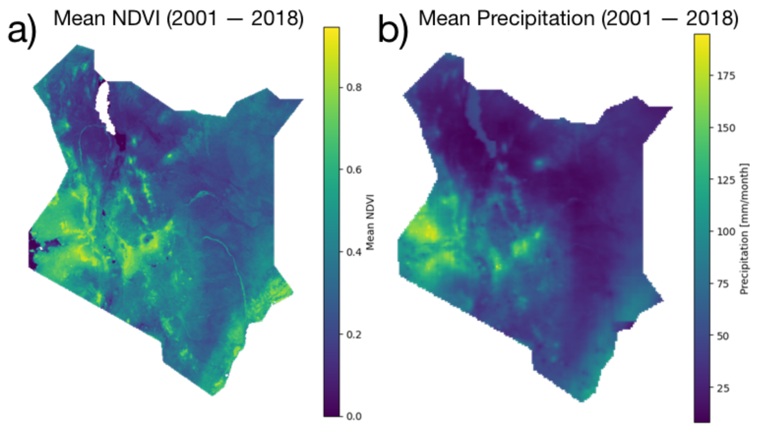
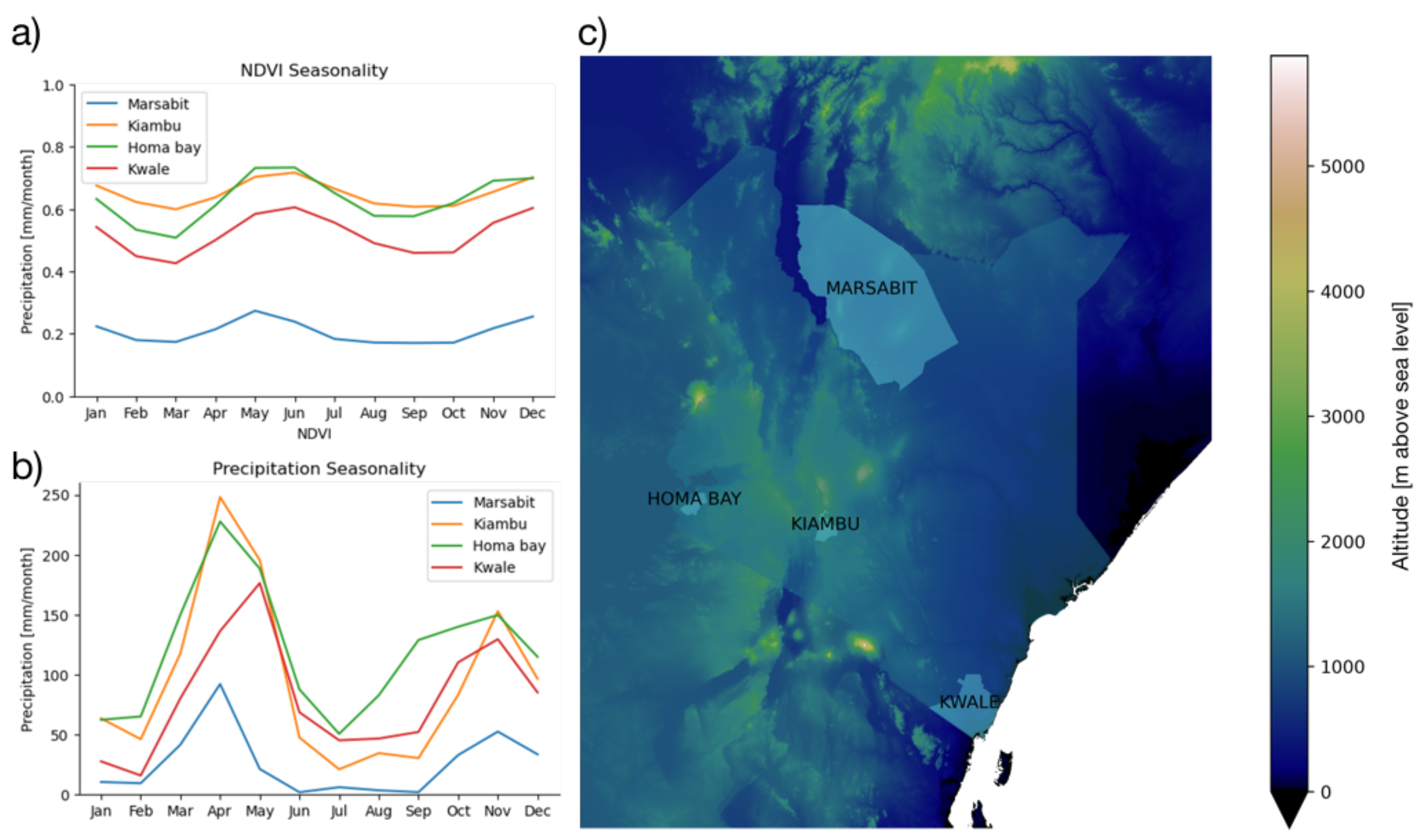
2.1. Study Area

We evaluate our approach in Kenya, for the region bounded by latitudes (−5.202, 6.002${}^{\circ }$ N) and longitudes (33.501, 42.283${}^{\circ }$ E). This covers an area of 580,367 km${}^2$ and contains diverse hydro-climatic regimes. The arid and semi-arid lands cover 80% of the country’s landmass and see on average less than 500 mm of rainfall per year [29]. The semi-humid areas are mostly mid-elevation areas where productivity is highly variable with maize being the dominant crop grown. The highly productive humid regions cover both sides of the Rift Valley, the valley floor, the humid lowlands on the shores of Lake Victoria, and a thin strip on the coastal areas in the South East of the country (Network [29]—see Figure 1b). Some coastal areas receive over 500 mm and the Western and central areas receive over 700 mm of annual rainfall. The mean annual NDVI closely follows this pattern, showing a thin strip of green areas along the coast, either side of the Rift Valley and around the shores of Lake Victoria (see Figure 1a). In contrast, the dry Turkana Channel shows low mean NDVI conditions.

When we aggregate the conditions at a pixel level to different counties we can see the diversity in conditions across the country. In Figure 2, we consider the seasonality of precipitation and NDVI for four different counties. Marsabit is a dry county in the North West of Kenya. Kiambu is a central county, adjacent and North of Nairobi. This is a highly productive region of Kenya. Homa Bay is on the shores of Lake Victoria and the wettest of the four counties we display below. Finally, Kwale is in the far South East corner of Kenya, a coastal county.

2.2. Data

2.2.1. Target Variable: Vegetation Condition Index

Remotely sensed vegetation has been used in many studies as a proxy for the agricultural drought conditions. The Normalised Difference Vegetation Index (NDVI) is a spectrally derived indicator of vegetation biomass and is commonly used for measuring agricultural drought conditions [13]. The NDVI product used by the NDMA is derived from MOD13Q1 and MYD13Q1 NDVI collection 5 products and has been processed using the methods described by Klisch and Atzberger [15]. These preprocessing steps involve the application of a modified Whittaker smoother in order to provide consistent, denoised images (removing clouds and poor atmospheric conditions) every 7 days. The data are processed to a 1 km resolution and to a 250 m resolution. Since we downscale the data to a lower resolution of the precipitation product, we use the 1km product here. This dataset is available from 2001 until today, for the analysis that follows we used 2001–2018.

The Vegetation Condition Index (VCI) is an anomaly index that ranks the observed NDVI for that pixel-time, when compared to all historical NDVI observations. The highest NDVI observation for that pixel-time in the historical dataset is given a VCI score of 100. The lowest NDVI observation for that pixel time is given a VCI score of 0. It is computed as in Kogan [30]. In this way we are linearly scaling the observed NDVI between the minimum observed NDVI (0) and the maximum observed NDVI (100) for that pixel-time.

$${\mathrm{VCI}}_i=100\ast \frac{{\mathrm{NDVI}}_i-NDV{I}_{\min ,i}}{{\mathrm{NDVI}}_{{\max }_i}-NDV{I}_{\min ,i}}$$

(1)

The VCI is calculated specifically for each pixel and each time. Therefore, the seasonality is removed, such that the VCI value reflects the current condition relative to prior conditions, scaled to between [0, 100]. One important thing to note is that values outside of the [0–100] range can be found if the observed NDVI is greater/smaller than the previous maximum/minimum value. We derived the VCI metrics, defining maximum and minimum NDVI values, from the timesteps in the historical period (2002–2015). This ensures consistency with the current approach used by NDMA.

To compare results with existing literature [31] we have chosen to predict both the 3 month rolling average VCI (VCI3M), as well as the monthly VCI (VCI1M) one month ahead in time. The VCI3M metric reflects the most damaging agricultural droughts, those occurring over an entire season. Therefore, VCI3M is the metric used for quantifying agricultural drought by the National Drought Management Authority (NDMA).

2.2.2. Input Variables

In

Table 1. Variables included in the model. Note that we include 11 features for the month of the year, since including 12 would create features with perfect collinearity.

Raw Spatial Resolution (Prior to Resmapling)	Feature	Model Usage	Source
Precipitation	X_dynamic	CHIRPS [32]	5 km${}^2$
Potential Evaporation (pev)	X_dynamic	ERA5 [33]	30 km${}^2$
Evaporation (e)	X_dynamic	ERA5 [33]	30 km${}^2$
Soil Moisture (4 Levels) (swvl {1, …, 4}	X_dynamic	ERA5 [33]	30 km${}^2$
Altitude	X_static	NASA SRTM [34]	0.03 km${}^2$
Month of Year	X_dynamic	—	—
Vegetation Condition Index (VCI {1, …, 3})	X_dynamic, y	MODIS Reflectances processed according to [15]	1 km${}^2$

, we list the variables that were included as input to the models. These variables are split into dynamic (X_dynamic) variables and static attributes for each pixel (X_static). We thereby condition the response of vegetation health (VCI) (y) to hydro-meteorological variables (X_dynamic) on static attributes (X_static) that do not change over time but vary spatially. The latter attributes include soil type and altitude, as well as the mean conditions for each dynamic variable (hydro-meteorological signatures). The idea is that we communicate to the model how different locations will respond differently to dynamic forcings. Therefore, we are learning a mapping from the forcing variables (X_dynamic) to the target variable—VCI (y), which varies conditional upon the pixel attributes (X_static). These pixel attributes could, in principle, be measured anywhere globally, since the datasets that they are derived from are globally available. These input features were normalised by removing the mean and dividing by the standard deviation calculated in the training period for each pixel. In order to describe the changing conditions elsewhere we took a naive approach. We provided the model with a spatial mean of each variable at that timestep. For example, there is one value describing the mean precipitation for each timestep across every pixel ($spatial\_mean\_precip$).

2.2.3. ERA5 Reanalysis

ERA5 is ECMWF’s most recent reanalysis product. Reanalysis data combine models and observations using data assimilation to provide the best estimate of hydro-meteorological variables over the Earth [33]. ERA5 has global spatial coverage for 1979 till present at 137 pressure levels (vertical resolution) on an hourly time step. The spatial resolution is 0.31 deg [33]. For this study we use the spatial fields for Potential Evaporation, Evaporation, and Soil Moisture (Level 1–4).

As far as we are aware, ERA5 variables have not yet been validated over Kenya. ERA Interim, the precursor to ERA5 soil moisture has been shown to reproduce observed surface variability, however it overestimated soil moisture, especially in drylands [35]. ERA Interim Soil Moisture has been used by other studies in the region [36]. Tall et al. [37] validated precipitation and incoming short-wave radiation in Burkina Faso using in situ measurements. They found that ERA5 was better able to reproduce observations of both precipitation and incoming short-wave radiation than ERA Interim.

2.2.4. CHIRPS Precipitation

Climate Hazards Group InfraRed Precipitation with Station data (CHIRPS) is the precipitation product we used for our experiments [32]. CHIRPS is a quasi-global (50${}^{\circ }$S—50${}^{\circ }$N) daily precipitation product produced at 0.05 deg spatial resolution. The data combine in situ station observations and satellite precipitation estimates based on Cold Cloud Duration (CCD). The data have been validated against in situ measurements and other gridded data products [32]. Furthermore, it has been used extensively in drought-related studies in the region [38,39,40].

2.2.5. NASA SRTM

We used the 1-arc second Shuttle Radar Topography Mission (SRTM) digital elevation model (DEM) to derive altitude as a static predictor variable in our experiments [34].

2.3. Models

To forecast VCI, we utilise deep learning techniques often used by hydrologists for rainfall-runoff modelling, namely the Long Short Term Memory Network (LSTM) [24,25,41,42,43]. These models can be considered data-driven state-space models [44], updating an internal state vector through time by incorporating new information at each timestep. The state vector is then used to make a prediction of the target variable at that time step.

The standard LSTM architecture was introduced by Hochreiter [45], and has been described in a number of other hydrological contexts [42,46,47]. For the purposes of this paper we refer the reader to these references rather than repeating the standard LSTM conception here.

We also seek to test the Entity-Aware LSTM (EA LSTM) developed by [23], which fixes the input gate in time, only using static attributes (pixel specific properties) to determine which information flows from input data to the state-vector. This reduces the number of weights in the model and, therefore, should be considered a regularisation technique.

To contextualise and benchmark the LSTM based performances, we compare against a single hidden layer multi-layer perceptron (a fully connected neural network). This network is made up of an input layer, a hidden layer and an output layer. The hidden layer has a ReLU activation function and outputs a vector equal in size to the hidden size of the LSTMs (i.e., 64 values). We compare against this model as a simpler model architecture that does not take into account the inductive bias towards time-series data exhibited by the LSTM [45].

We also compare model performances against a persistence baseline. This baseline predicts that the target month VCI ($y_t$) will be the same as the previous month VCI ($y_{t-1}$). This logic can be summarised as ‘predict no change from the previous timestep’. We compare the models using both RMSE and R${}^2$ for the monthly data in the hold-out test period (2016–2018).

2.4. Experimental Setup

All data have been spatially regridded to the same spatial resolution as the ERA5 product (30 km${}^2$) using bilinear interpolation. The data are also temporally resampled to a monthly resolution. Therefore, we have one value for each variable, each pixel at each month. The analysis is conducted on monthly resolution data in order to account for the varying update frequencies of the input data and to ensure reasonable run times for Kenya-wide experiments.

We use the previous three months of dynamic data as input to our models. We use information from times $t-3$, $t-2$, $t-1$ as input to predict VCI at time t (one time-step ahead forecasting). We found that information prior to three months before the target time could be dropped without penalising performance, thereby speeding up training time and reducing the number of input features.

Models were trained using the smooth L1 loss function. The smooth L1 loss function, also known as the Huber loss function, was used with $\delta =1$. The smooth L1 loss is less sensitive to outliers than the mean squared error loss. This is because the error is linear when greater than $\delta$, but squared between [−1, 1]. This has been shown to speed up training times and to prevent exploding gradients [48]. Models were trained for a maximum of 100 epochs with a stopping criterion of 10 consecutive epochs without performance improvement (measured by the smooth L1 loss on the validation data).

$$\mathrm{loss}(x,y)=\frac{1}{n}\sum _i{z}_i$$

(2)

where $z_i$ is given by:

$$z_i=\left\{\begin{array}{cc}0.5{\left(x_i-y_i\right)}^2,\hfill & \mathrm{if}\left|x_i-y_i\right|<1\hfill \\ \left|x_i-y_i\right|-0.5,\hfill & \mathrm{otherwise}\hfill \end{array}\right.$$

(3)

All models were trained on the period 2002–2015 and tested on the period 2016–2018. We split the training data into training and validation sets. We trained a single LSTM or EA LSTM model using data from all pixels. Therefore, we learn a single model for all of Kenya, testing the ability of these models to make predictions across diverse contexts. This is in contrast to other models that have sought to predict VCI in different regions of Kenya, which have traditionally refit each model to each location [31].

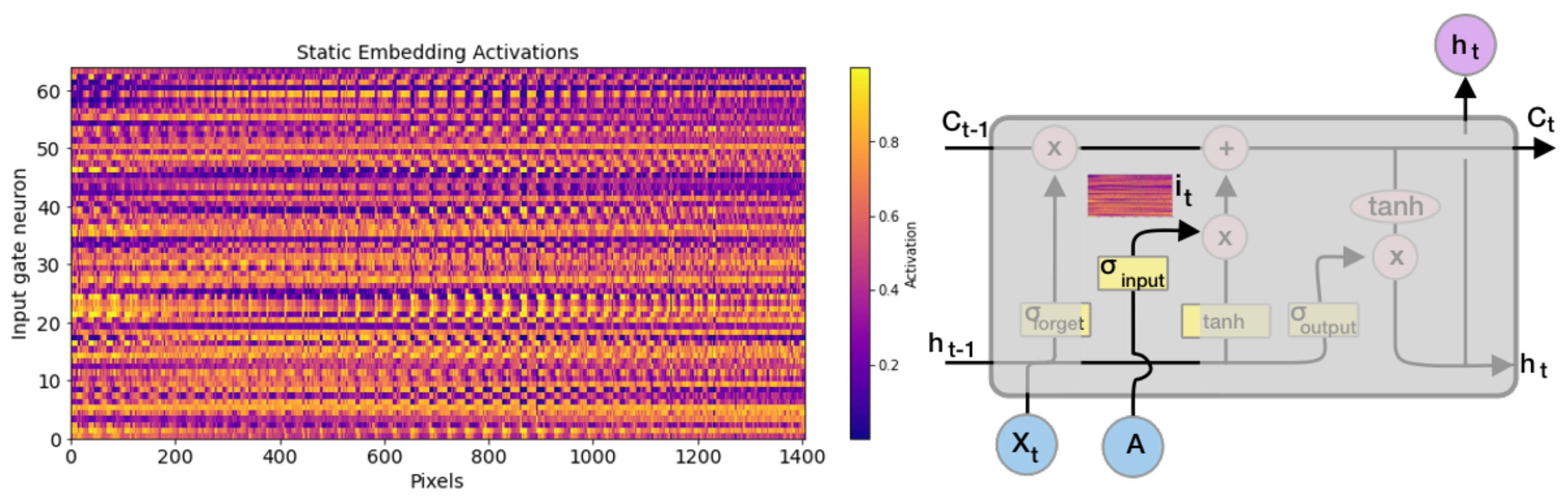
2.5. Interpreting the Models

To provide a physical interpretation of model structure and results we took two approaches, detailed below. The first approach is similar to that taken by Kratzert et al. [23]. Using cluster analysis we interpret how the model has learned to utilise the static features—those features that vary over space but not time (Table 1)—to group together similar vegetation health responses to the dynamic forcings. The second approach estimates the contribution of each input feature to the prediction for a given observation (x–y pair). This method is translated from game-theoretic approaches to machine learning [49] and gives a measure of feature importance with respect to a particular prediction.

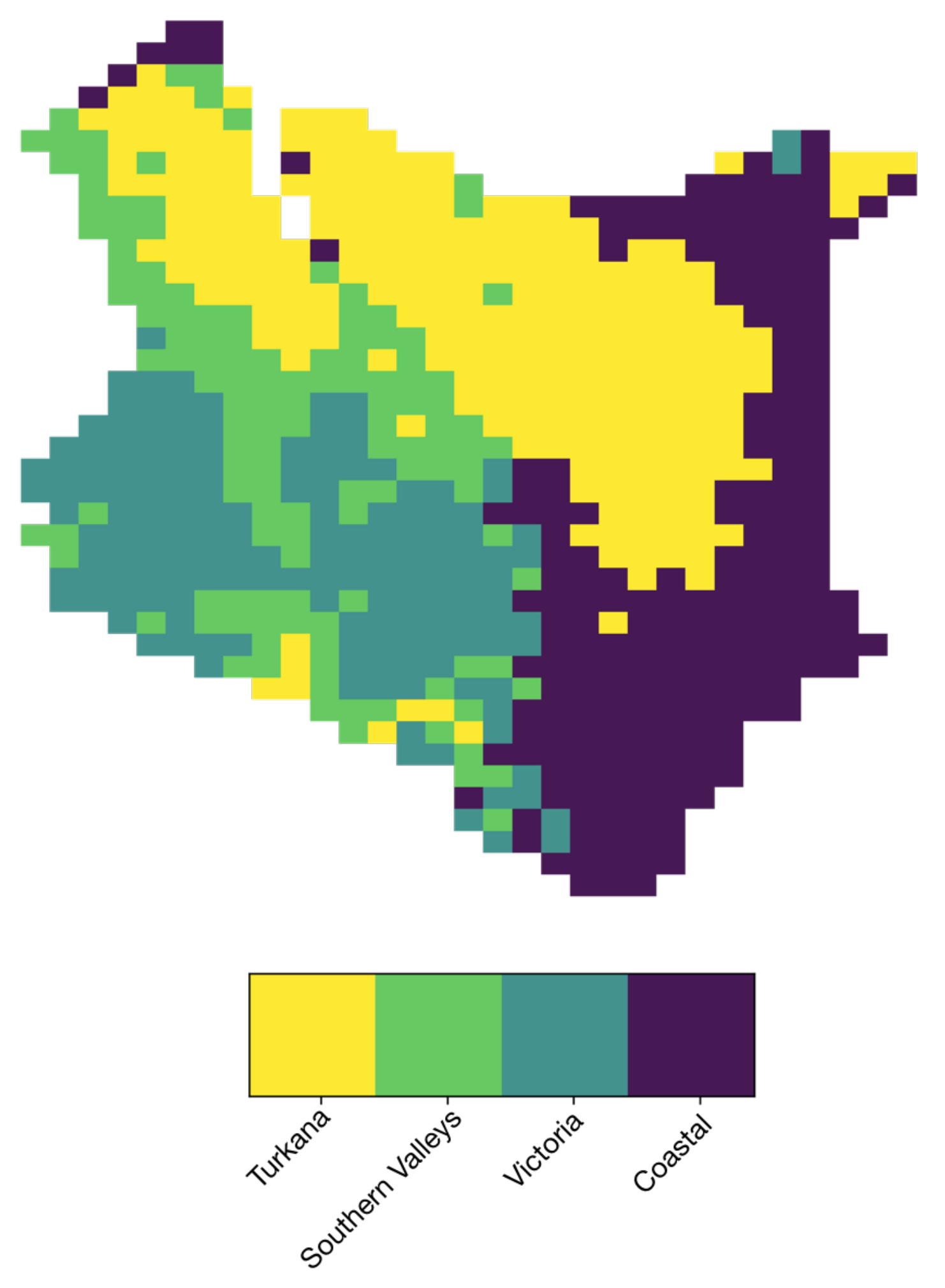
2.5.1. Clustering Analysis of the Static Embedding Layer

The Entity Aware LSTM learns a mapping of the x_static data (${\mathbb{R}}^{14}$) to the learned, higher-dimensional space (${\mathbb{R}}^{64}$) (the “embedding”) for each pixel (the column vectors of the matrix seen in Figure 3). This reflects how the model prediction of VCI (y) is conditioned on the pixel attributes ($x_{static}$). The result is a set of weights (valued [0, 1]) controlling how much information is passed from the dynamic data to the cell memory ($C\left[t\right]$) passing through each cell of the LSTM sequence.

What the model is learning, therefore, is how the $x_{static}$ data alters the response of vegetation health (VCI) to the dynamic data. This extends [23] by applying their methodology but in a different hydrological context. Rather than reflecting the grouping of hydrological catchments, we are grouping pixels to produce a data-driven classification of vegetation health regimes. These clusters highlight areas of similar vegetation health responses to dynamic forcing (e.g., precipitation).

By clustering the output of the static embedding layer (${\mathbb{R}}^{64}$) we can visualise the areas where vegetation health responds similarly to inputs. These can be inspected visually to determine whether the spatial patterns that the model represents are qualitatively similar to known physical distributions of agro-ecological zones.

We test the hypothesis that the EA LSTM model is able to group together similar pixels. We expect that pixels with similar vegetation health responses use similar parts of the network.

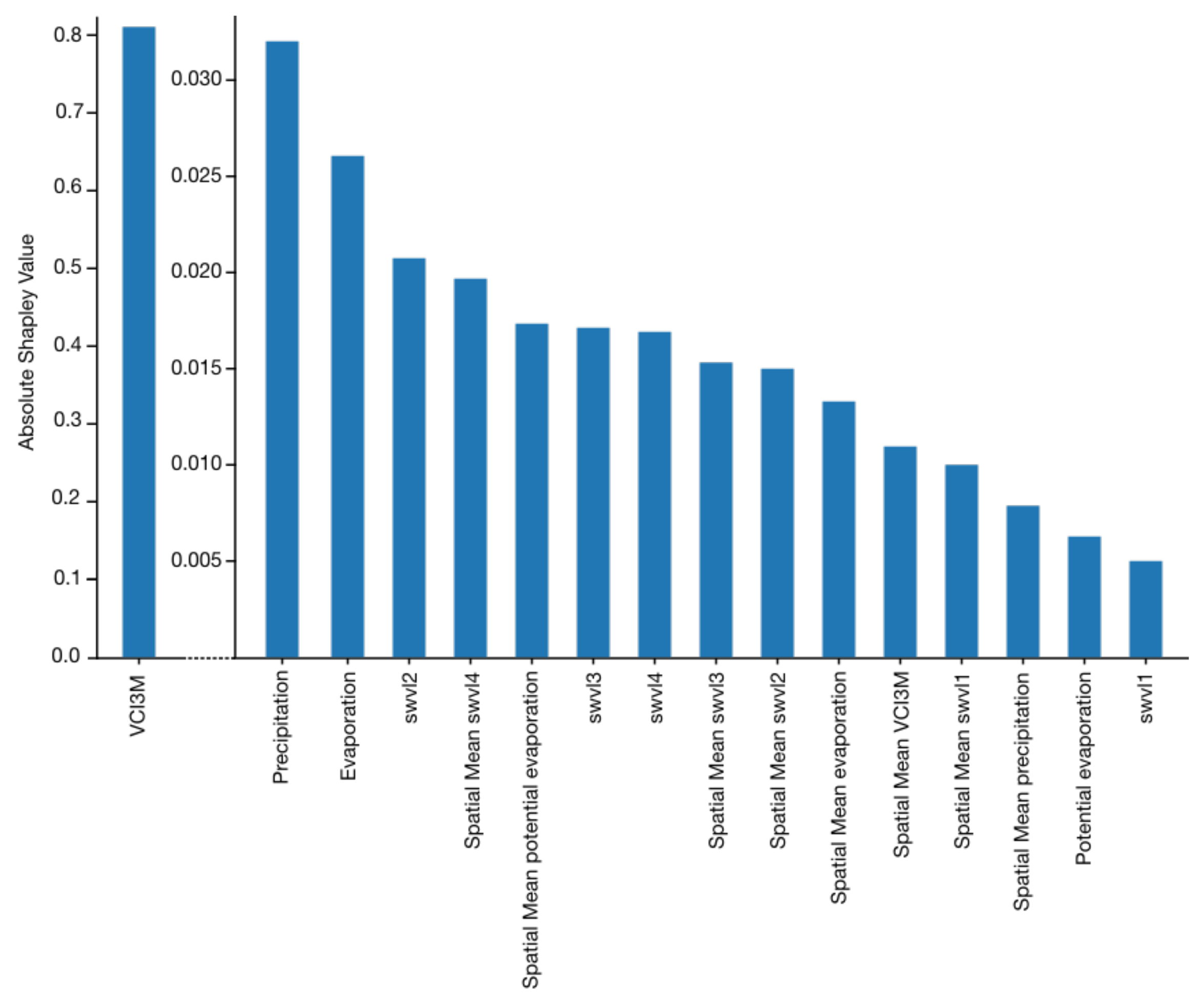
2.5.2. Determining Feature Importance

We also estimate the relative importance of different catchment attributes. We calculate Shapley values [50], which reflect the instance-wise contribution of each input feature to a specific prediction.

We first calculate the difference between the prediction for the specific instance we want to explain and a baseline prediction (the $\delta y$, or payout).

$$\delta y=\widehat{y}-{\widehat{y}}_{baseline}$$

(4)

We want to assign the $\delta y$ to each of the input features (our dynamic and static input features). The output values can contribute both positively and negatively to the model’s prediction.

We calculate Shapley values using the DeepLIFT method [51] implemented using the SHAP library [49]. Three inputs are needed to calculate the Shapley values:

• A baseline output to compare our predictions to;
• Our model prediction we want to explain;
• The values for the features that we want to assign importance to.

For our baseline output we follow Lundberg and Lee [49], and use the average of 100 sampled model outputs from the training dataset, as baseline model. Intuitively, we are asking: what would the model predict with no information, and how would the specific features in a datapoint change the model’s prediction from the no-information prediction? For our analysis, a global sensitivity measure is calculated for each feature and each pixel by taking the average absolute Shapley value.

3. Results

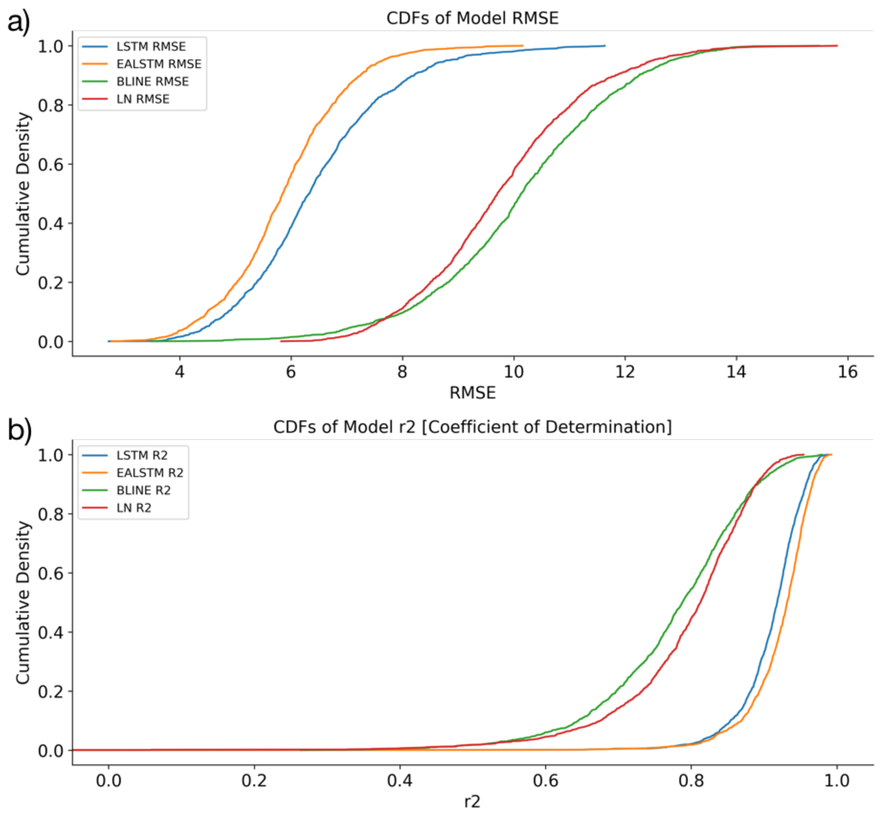
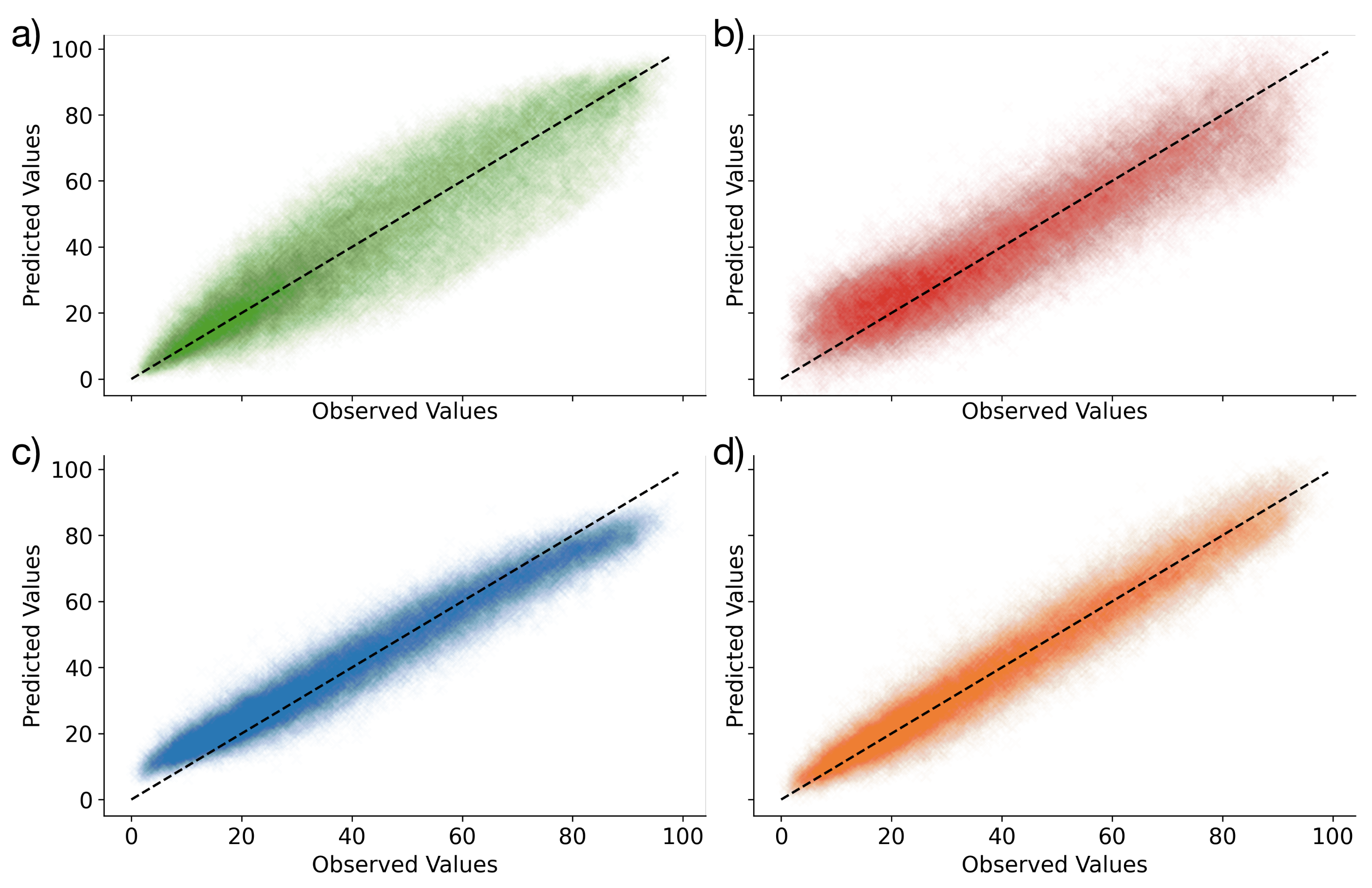
3.1. Model Performances

Results comparing the LSTM approaches, our persistence baseline and a simple fully-connected feed-forward neural network are summarised in Figure 4 and

Table 2. Average performance metric for each pixel in the domain and for each time in the hold-out test period (2016–2018). The best in class results are highlighted in bold.

	Error Metric	Persistence (BLINE)	Neural Network (LN)	LSTM	EA LSTM
VCI3M	RMSE	10.20	9.81	6.46	5.88
	R${}^2$	0.86	0.88	0.95	0.95
VCI1M	RMSE	18.84	25.68	13.23	13.23
	R${}^2$	0.66	0.14	0.83	0.82

. This shows the cumulative density functions of the models and the persistence baseline (BLINE). All three models were trained on the same input data and their performance evaluated on the hold-out test set, using all months from 2016–2018.

• The LSTM and EA LSTM performances are extremely similar;
• Both the EA LSTM and LSTM significantly outperform the persistence baseline;
• The simple feed-forward neural network performs very similarly to the persistence baseline;
• All models predict the temporally smoother VCI3M better than VCI1M.

The cumulative distribution functions (Figure 4a) show the performance of the model RMSEs when predicting VCI3M. We can see that the LSTM models significantly outperform both the persistence baseline and the simple feed-forward neural network. Interestingly, the simple neural network seems to perform worse than the persistence baseline. This is shown by the long tail of model performances. The same is observed for R${}^2$ (Figure 4b).

From the scatter plots shown in Figure 5, one can see that the predictions of the EA LSTM group are closely scattered around the one-to-one line, whereas both the LSTM and the simple neural network show some bias at low or high VCI values.

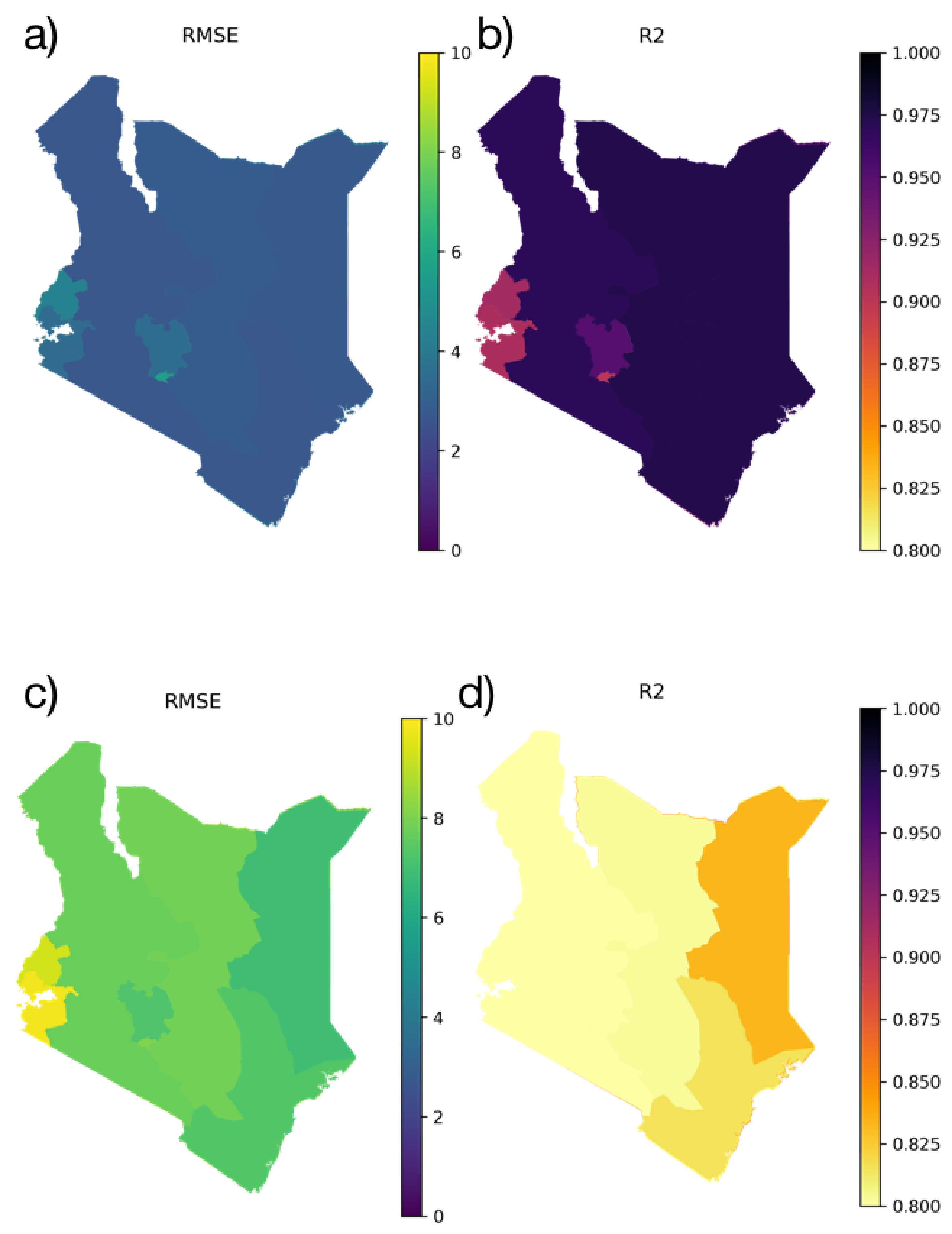
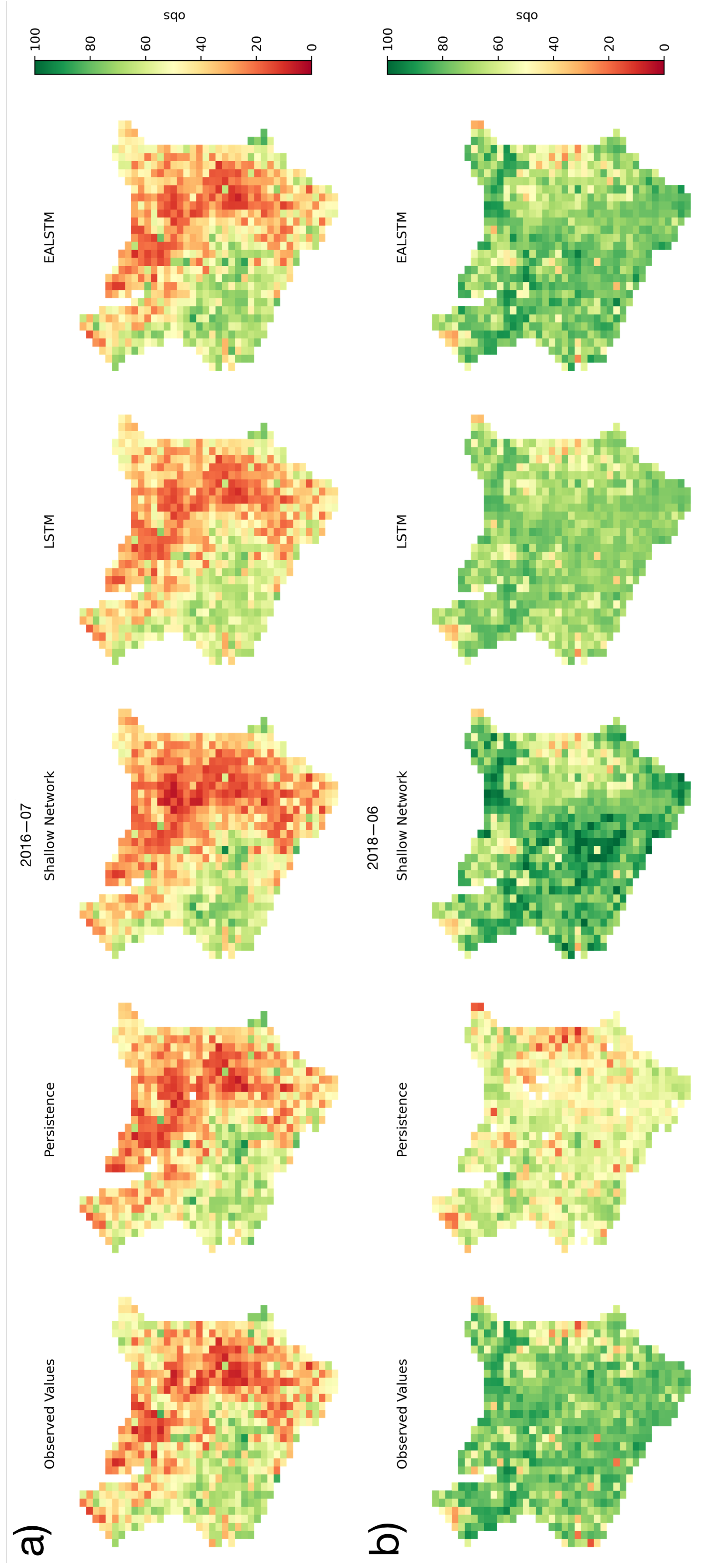
3.1.1. Spatial Distribution of Model Results

When we compare spatial performances against the persistence based model in Figure 6 we can see that the EA LSTM performs well across Kenya. However, the baseline model fails in the highly productive regions, since the vegetation condition varies rapidly in time, such that the previous month is not as good a predictor of the following month in the more productive regions of Central Kenya, surrounding Nairobi, and near to Lake Victoria. Overall, the patterns show that the EA LSTM is able to significantly outperform the persistence baseline across Kenya.

In Figure 7 we show model predictions for June 2018. What is interesting about June 2018 is that the persistence model significantly underpredicts the VCI. In contrast, with the information from the hydro-meteorological inputs, the LSTM based models were able to more accurately predict the degree of greening. The period starting in June 2018 was an extremely wet month across much of the country, with associated positive vegetation health anomalies [52].

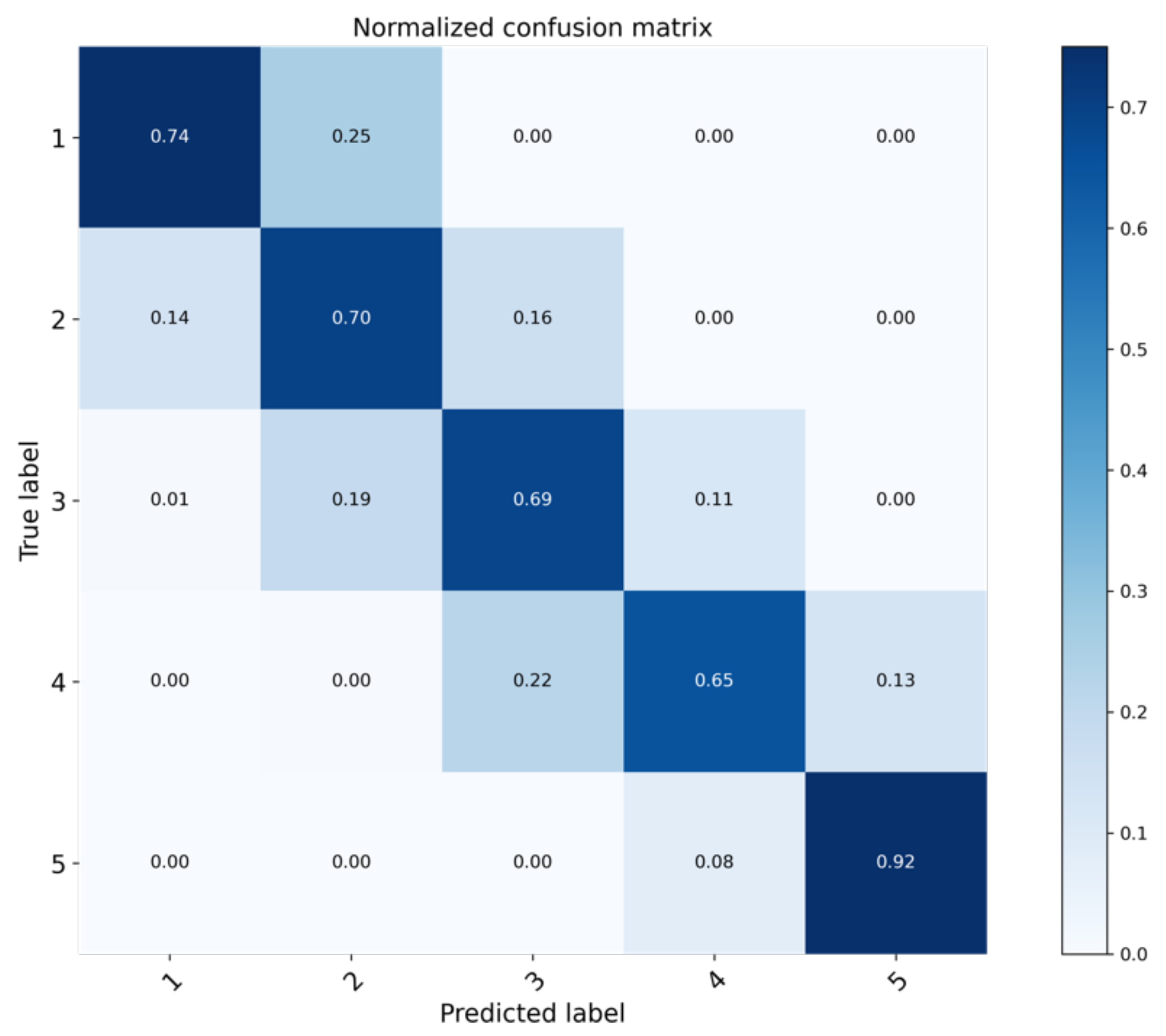
3.1.2. Performance on Drought Classes

The models are trained as regression models, to predict the VCI as a continuous variable. However, when the VCI is used in operation by the NDMA and other drought agencies, the agencies are often interested in specific drought classes, such as “extreme” or “severe” drought [53]. Drought classes and thresholds are also used in index insurances, where the correct modeling of the worst conditions matters most [54]. To test the model performance across these drought classes we present the confusion matrix below, where we use the drought classes described by Klisch and Atzberger [15], which are also used by the Kenyan NDMA. What we find is that the LSTM models are able to predict well across the distribution for VCI3M. The EA LSTM predicts the correct drought class with an accuracy of 78.3% and errors only occur between two adjacent classes. In the analysis that follows, we only show the EA LSTM model performances.

The confusion matrix in Figure 8 shows the EA LSTM performance across all drought classes. Overall, the EA LSTM is capable of detecting drought conditions one month ahead. Interestingly, the most critical drought class (“extreme”) is predicted with higher accuracy compared to the other drought classes, except the class 5. This demonstrates the possibility of using the LSTM to monitor and predict negative anomalies, even in those circumstances where the VCI score is less than 10 (see

Table 3. The Vegetation Deficit Index classes defined by Klisch and Atzberger [15].

VCI3M Limits	Description	Value
$x<10$	Extreme Vegetation Deficit	1
$10<=x<20$	Severe Vegetation Deficit	2
$20<=x<35$	Moderate Vegetation Deficit	3
$35<=x<50$	Normal Vegetation Conditions	4
$x<=50$	Above normal Vegetation Condition	5

). We can see that 74% of the values were correctly classified, and 25% of values were incorrectly classified on these negative anomalies.

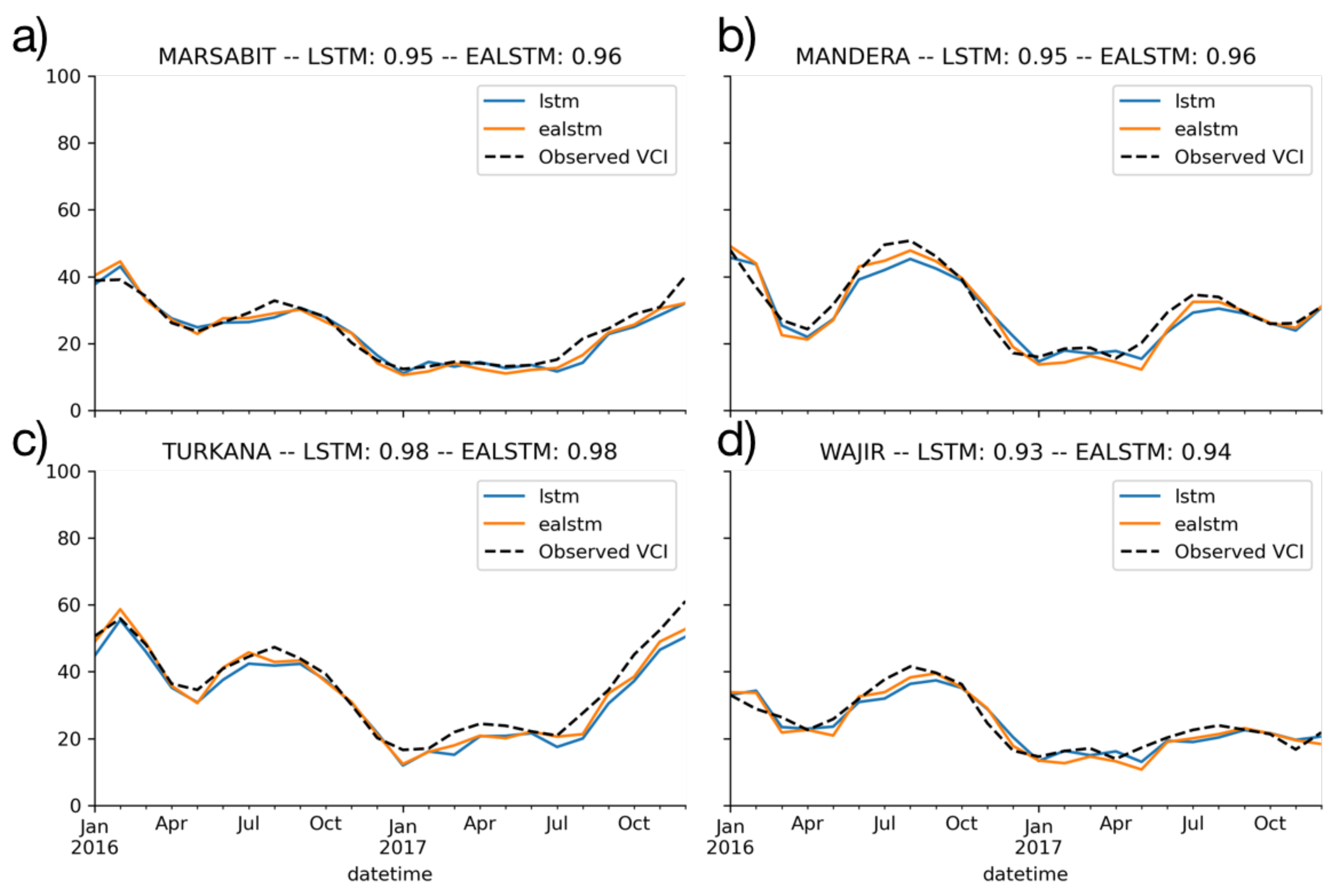
3.1.3. Comparison with State of the Art

In addition to comparing against a persistence baseline, we compared our models to the NDMA model, developed by researchers at the NDMA [31]. These published results were chosen as a useful comparison because we are directly predicting the same target variable, and because we are interested in the application of these methods to operational drought monitoring scenarios. Using indices derived from temperature, vegetation health, evapotranspiration, potential evapotranspiration, and precipitation, the NDMA model consists of an ensemble of 111 fully-connected neural networks and support vector regressions.

Our results are presented in Table 4. The only reported test results of R${}^2$ are from 2016–2017, and therefore, we only used those years and recalculated our VCI3M R${}^2$ scores. In addition, the NDMA model predicts a single VCI3M value per district and is trained on that district. To compare their model with ours, we took a district-wide mean of our pixel-wise predictions.

Table 4. Performance (measured using R${}^2$) over selected arid and semi arid land districts (following Adede et al. [31]) for the period 2016–2017. Best in class highlighted in bold. The underlying timeseries from which these results are calculated can be seen in Figure 9.

District	Adede et al. [31]	Persistence	LSTM	EA LSTM
Mandera	0.94	0.66	0.95	0.96
Marsabit	0.94	0.74	0.95	0.96
Turkana	0.91	0.74	0.98	0.98
Wajir	0.96	0.84	0.93	0.94

Table 4. Performance (measured using R${}^2$) over selected arid and semi arid land districts (following Adede et al. [31]) for the period 2016–2017. Best in class highlighted in bold. The underlying timeseries from which these results are calculated can be seen in Figure 9.

District	Adede et al. [31]	Persistence	LSTM	EA LSTM
Mandera	0.94	0.66	0.95	0.96
Marsabit	0.94	0.74	0.95	0.96
Turkana	0.91	0.74	0.98	0.98
Wajir	0.96	0.84	0.93	0.94

Our models are competitive with the NDMA ensemble model, but produce much more spatially granular predictions. This is particularly encouraging because during the 2016–2017 period being compared, significant droughts were recorded in Wajir [55] and in Turkana and Marsabit Uhe et al. [40]. These conditions represent the conditions in which we most want the models to perform well.

It is important to emphasise the differences between these models. The first is that Adede et al. [31] train an ensemble of models, whereas we train one model. This offers the potential to provide confidence intervals, however the reported results show only the ensemble mean prediction. The second is that the spatial granularity of our predictions are much higher than the NDMA model, where predictions are produced at a district level. We, therefore, adapted our results to compare directly with the published results. Finally, our model is applicable across the whole country, rather than being specifically trained for each of these four counties.

3.2. Interpreting the Static Embedding

One appealing and unique feature of the EA LSTM is the static embedding layer. We learn a unique input-gate vector for each pixel in the data. These are the columns in the matrix in Figure 3. Yellow colours indicate values close to 1 indicating that the cell is activated and all of the information from the dynamic data corresponding to this cell is contributing to the prediction of this pixel’s VCI. These values are a function of the pixel’s static data.

The static embedding permits us to test whether the model was learning physically realistic groupings of the pixels, based on their vegetation health response (VCI) to changes in hydro-meteorological variables. We do this by clustering the matrix in Figure 3 using k-means clustering with a Euclidean distance criterion. This reduces the dimensionality of the ${\mathbb{R}}^{64}$ embeddings for each pixel to a lower dimensional representation. We chose k = 4 because there are roughly four (4) major bioclimatic zones in Kenya (Figure 11 of Livelihood Zones p. 15 or Figure 5 of Agro-Ecological Zones p. 10 [29]). To test whether these groupings are physically realistic we plotted the pixel clusters geographically (Figure 10).

In Figure 10, we plot the output of the clustering of the learned model embedding. These clusters represent broad hydro-ecological zones in Kenya. The Turkana Channel region (shown in purple) is very arid and hot.

This method offers the opportunity to derive data-driven vegetation health regimes, showing the diversity of different vegetation responses to hydro-meteorological drivers. This analysis could be used to better understand the diversity of vegetation health responses in diverse hydro-climatic regimes in Kenya, and also help to identify areas that behave differently.

What this analysis offers most importantly, however, is evidence that the model is learning physically realistic groupings of vegetation health regimes. This offers an understanding that the model is not only an accurate predictor, but that it is making predictions for physically-plausible reasons that we can interrogate by visualising this learned matrix [21].

3.3. Measuring the Contribution of Dynamic Features

We calculated the mean absolute Shapley value [49] to give an estimate of the global feature importance. This allows us to identify which features are significantly contributing to the predictions.

The autoregressive component is extremely important for the models (Figure 11). This reflects the behaviour of 3 month moving average vegetation health anomalies (VCI3M). They tend to persist from month to month, exhibiting a high degree of autocorrelation. However, the model significantly outperforms the persistence based model by incorporating new information from the other hydro-meteorological input features (X_dynamic), as shown in Figure 4.

Figure 11 shows that other dynamic features also contribute to the predictions, albeit a smaller absolute contribution than the autoregressive component. Precipitation and evaporation features offer additional information to the model beyond this autoregressive component. This makes sense, since the model will need to learn a rudimentary approximation of the water balance, using the precipitation to describe water entering the land surface and evaporation describing water leaving the land surface. This learned water balance is useful for the EA LSTM to estimate vegetation health. It is also interesting that soil water volume—level 2 (swvl2) is the most informative soil water volume metric. Level 2 corresponds with water between 7 and 28 cm.

Ultimately, these figures give us faith that the model is learning physically realistic signals, incorporating information from precipitation and evaporation to calculate the contribution of available water to the vegetation health.

4. Discussion and Conclusions

In this study, we have explored the efficacy of two LSTM-based architectures for vegetation health forecasting. We find that these recurrent neural network architectures outperform a shallow neural network and the persistence baseline. The most likely explanation for the improved performance of the LSTM compared with the shallow neural network is the inductive bias towards modelling time-series [45]. The LSTMs are competitive with the published results for the ensemble of models developed by the NDMA [31], while also having significantly greater spatial resolution. Although there are difficulties in directly comparing between different methods, because of differences in input datasets, training periods and experimental designs, it is important to place these results in the broader context of previously completed research. We test our models across the whole of Kenya, and demonstrate the LSTM models are able to make accurate predictions across the country, despite the diversity of environmental conditions.The forecasts are also robust across the distribution of VCI values. We tested the model’s ability to predict the VCI classes defined by Klisch and Atzberger [15]. We are able to perform well across the distribution and also for the most relevant drought classes “severe” and “extreme vegetation deficit” that trigger payouts under NDMA’s Disaster Contingency Funds and the Human Safety Net Program.

The results of this study demonstrate that methods used elsewhere in hydrology offer potential for vegetation health forecasting, and in turn offer opportunities for EO-based drought early warning systems.

We have also demonstrated that deep learning models offer the potential to combine information from earth observation data with meteorological variables (such as precipitation and temperature) from reanalysis data. These datasets are globally available, and demonstrate the power of deep learning techniques for deriving accurate forecasts of variables of interest (in our case vegetation health). This can be particularly valuable in cases where we lack the physical intuition to accurately model these variables using process-based models, as is the case for vegetation health. It is also valuable because it allows us to generate accurate forecasts in regions of the world where in situ data are difficult to access or even non-existent. Moreover, it is easy to envision including either numerical weather forecasts or (user-defined) weather scenarios into our framework.

One of the key criticisms of deep learning methods is the fact that the models are often uninterpretable [21]. We attempted to address this shortcoming by using two methods to determine what the LSTM-based models were learning. The first was the clustering methodology proposed by [23]. Using the learned representation of the pixel attributes, we were able to produce spatial clusters of distinct vegetation health regimes. These data-driven clusters of vegetation health regimes are qualitatively realistic and provide evidence that the model is learning sensible relationships that can be interpreted physically. Secondly, we used gradient based methods to estimate Shapley values [51], determining the relative contribution of input features to a specific prediction. These show that the autoregressive component contributed the largest amount of information to the EA LSTM. It is clear that precipitation and evaporation also contributed, however, the importance of these variables was small when compared with the previous month’s vegetation condition. Further research should consider how the sensitivity to different features varies with different lag-times and across space.

We were able to use the Shapley values to make practical decisions about our experiments and model architecture. We experimented with feeding a longer time-series to the model, but using the calculated Shapley values we determined that the LSTMs did not use information from more than 3 months before the prediction date. Reducing the length of the input time-series reduced training time without penalising performance.

Exploring methods for interpreting deep learning time-series models is an area of active research [56]. In this study we have demonstrated two approaches that help us to understand what the model is learning and there is good evidence that these relationships are physically realistic. One might also want to determine the contribution of features over time, to interpret the seasonal patterns, and the contribution over space, to interpret the spatial patterns. Moreover, alternative feature sensitivity metrics exist, such as integrated gradients [57]. Future work should consider how robust feature importance scores are to different calculation methods.

There are a number of avenues for further exploration. Firstly, as we are most interested in drought conditions (VCI < 35) we can experiment with weighting these observations more heavily, forcing the model to pay more attention to these observations when performing the backward pass. Secondly, it would be interesting to explore the use of hydro-meteorological forecasts (rainfall and temperature) as inputs to the model. The use of (probabilistic or scenario-based) forecasts would potentially also offer the possibility of extending the forecast horizon beyond the current one month limit. This offers two benefits, firstly, it provides an estimate of model uncertainty for the one month forecasts. Secondly, we are able to make forecasts over a longer time horizon.

This study has demonstrated the ability of recurrent deep learning models to predict a widely used agricultural drought index (VCI) derived from earth observation data. This confirms and extends other studies that show LSTM models are effective for hydrological modelling [23,42,46] and for combining the information from earth observation datasets with weather data [20]. We have explored two methods for interpreting these deep learning models and find that the results suggest we are learning physically realistic signals. Kenya has been struck by drought conditions in recent decades and it offers a location where these techniques can add significant value to decision makers in operational settings. However, the method and datasets we have evaluated exist globally, and it is the authors opinion that this method can be generalised to other locations. In this manuscript, we have presented evidence that our approach has the potential to provide useful information to drought management authorities in a timely manner. Furthermore, because the method, datasets and overall approach is location agnostic, there is the opportunity to test a similar approach elsewhere.

References

1. Wilhite, D.A.; Svoboda, M.D.; Hayes, M.J. Understanding the complex impacts of drought: A key to enhancing drought mitigation and preparedness. Water Resour. Manag. 2007, 21, 763–774. [Google Scholar] [CrossRef] [Green Version]
2. Van Loon, A.F. Hydrological drought explained. Wiley Interdiscip. Rev. Water 2015, 2, 359–392. [Google Scholar] [CrossRef]
3. Vicente-Serrano, S.M.; Beguería, S.; López-Moreno, J.I. A multiscalar drought index sensitive to global warming: The standardized precipitation evapotranspiration index. J. Clim. 2010, 23, 1696–1718. [Google Scholar] [CrossRef] [Green Version]
4. Spinoni, J.; Naumann, G.; Vogt, J.V.; Barbosa, P. The biggest drought events in Europe from 1950 to 2012. J. Hydrol. Reg. Stud. 2015, 3, 509–524. [Google Scholar] [CrossRef]
5. Nicholson, S.E. A detailed look at the recent drought situation in the Greater Horn of Africa. J. Arid Environ. 2014, 103, 71–79. [Google Scholar] [CrossRef]
6. Swain, D.L.; Tsiang, M.; Haugen, M.; Singh, D.; Charland, A.; Rajaratnam, B.; Diffenbaugh, N.S. The extraordinary California drought of 2013/2014: Character, context, and the role of climate change. Bull. Am. Meteorol. Soc. 2014, 95, S3. [Google Scholar]
7. Baudoin, M.A.; Vogel, C.; Nortje, K.; Naik, M. Living with drought in South Africa: Lessons learnt from the recent El Niño drought period. Int. J. Disaster Risk Reduct. 2017, 23, 128–137. [Google Scholar] [CrossRef]
8. Muller, M. Cape Town’s drought: Don’t blame climate change. Nature 2018, 559, 174–176. [Google Scholar] [CrossRef] [Green Version]
9. Zeng, N.; Yoon, J.H.; Marengo, J.A.; Subramaniam, A.; Nobre, C.A.; Mariotti, A.; Neelin, J.D. Causes and impacts of the 2005 Amazon drought. Environ. Res. Lett. 2008, 3, 014002. [Google Scholar] [CrossRef]
10. García-Herrera, R.; Díaz, J.; Trigo, R.M.; Luterbacher, J.; Fischer, E.M. A review of the European summer heat wave of 2003. Crit. Rev. Environ. Sci. Technol. 2010, 40, 267–306. [Google Scholar] [CrossRef]
11. Arias, P.; Bellouin, N.; Coppola, E.; Jones, R.; Krinner, G.; Marotzke, J.; Naik, V.; Palmer, M.; Plattner, G.K.; Rogelj, J.; et al. Climate Change 2021: The Physical Science Basis. Contribution of Working Group14 I to the Sixth Assessment Report of the Intergovernmental Panel on Climate Change; Technical Summary; Cambridge University Press: Cambridge, UK, 2021. [Google Scholar]
12. Rembold, F.; Meroni, M.; Urbano, F.; Csak, G.; Kerdiles, H.; Perez-Hoyos, A.; Lemoine, G.; Leo, O.; Negre, T. ASAP: A new global early warning system to detect anomaly hot spots of agricultural production for food security analysis. Agric. Syst. 2019, 168, 247–257. [Google Scholar] [CrossRef] [PubMed]
13. Svoboda, M.D.; Fuchs, B.A. Handbook of Drought Indicators and Indices; World Meteorological Organization: Geneva, Switzerland, 2016. [Google Scholar]
14. Sheffield, J.; Wood, E.F.; Chaney, N.; Guan, K.; Sadri, S.; Yuan, X.; Olang, L.; Amani, A.; Ali, A.; Demuth, S.; et al. A drought monitoring and forecasting system for sub-Sahara African water resources and food security. Bull. Am. Meteorol. Soc. 2014, 95, 861–882. [Google Scholar] [CrossRef]
15. Klisch, A.; Atzberger, C. Operational drought monitoring in Kenya using MODIS NDVI time series. Remote Sens. 2016, 8, 267. [Google Scholar] [CrossRef] [Green Version]
16. Brisson, N.; Gary, C.; Justes, E.; Roche, R.; Mary, B.; Ripoche, D.; Zimmer, D.; Sierra, J.; Bertuzzi, P.; Burger, P.; et al. An overview of the crop model STICS. Eur. J. Agron. 2003, 18, 309–332. [Google Scholar] [CrossRef]
17. Van Diepen, C.v.; Wolf, J.; Van Keulen, H.; Rappoldt, C. WOFOST: A simulation model of crop production. Soil Use Manag. 1989, 5, 16–24. [Google Scholar] [CrossRef]
18. Wilby, R.; Abrahart, R.; Dawson, C. Detection of conceptual model rainfall—Runoff processes inside an artificial neural network. Hydrol. Sci. J. 2003, 48, 163–181. [Google Scholar] [CrossRef] [Green Version]
19. Dawson, C.W.; Wilby, R. An artificial neural network approach to rainfall-runoff modelling. Hydrol. Sci. J. 1998, 43, 47–66. [Google Scholar] [CrossRef]
20. Shen, C. A Transdisciplinary Review of Deep Learning Research and Its Relevance for Water Resources Scientists. Water Resour. Res. 2018, 54, 8558–8593. [Google Scholar] [CrossRef]
21. Nearing, G.; Kratzert, F.; Sampson, A.K.; Pelissier, C.S.; Klotz, D.; Frame, J.; Prieto, C.; Gupta, H. What Role Does Hydrological Science Play in the Age of Machine Learning? Water Resour. Res. 2021, 57, e2020WR028091. [Google Scholar] [CrossRef]
22. Nay, J.; Burchfield, E.; Gilligan, J. A machine-learning approach to forecasting remotely sensed vegetation health. Int. J. Remote Sens. 2018, 39, 1800–1816. [Google Scholar] [CrossRef]
23. Kratzert, F.; Klotz, D.; Shalev, G.; Klambauer, G.; Hochreiter, S.; Nearing, G. Towards learning universal, regional, and local hydrological behaviors via machine learning applied to large-sample datasets. Hydrol. Earth Syst. Sci. 2019, 23, 5089–5110. [Google Scholar] [CrossRef] [Green Version]
24. Gauch, M.; Kratzert, F.; Klotz, D.; Nearing, G.; Lin, J.; Hochreiter, S. Rainfall–runoff prediction at multiple timescales with a single Long Short-Term Memory network. Hydrol. Earth Syst. Sci. 2021, 25, 2045–2062. [Google Scholar] [CrossRef]
25. Lees, T.; Buechel, M.; Anderson, B.; Slater, L.; Reece, S.; Coxon, G.; Dadson, S.J. Benchmarking data-driven rainfall–runoff models in Great Britain: A comparison of long short-term memory (LSTM)-based models with four lumped conceptual models. Hydrol. Earth Syst. Sci. 2021, 25, 5517–5534. [Google Scholar] [CrossRef]
26. Klotz, D.; Kratzert, F.; Gauch, M.; Sampson, A.K.; Klambauer, G.; Hochreiter, S.; Nearing, G. Uncertainty Estimation with Deep Learning for Rainfall-Runoff Modelling. arXiv 2020, arXiv:2012.14295. [Google Scholar]
27. FAO. Kenya at a Glance. Available online: https://www.fao.org/kenya/fao-in-kenya/kenya-at-a-glance/en/ (accessed on 12 December 2021).
28. Nicholson, S.E. Climate and climatic variability of rainfall over eastern Africa. Rev. Geophys. 2017, 55, 590–635. [Google Scholar] [CrossRef] [Green Version]
29. Network, F. Kenya Food Security: In Brief. 2013. Available online: https://fews.net/sites/default/files/documents/reports/Kenya_Food%20Security_In_Brief_2013_final_0.pdf (accessed on 12 December 2021).
30. Kogan, F.N. Application of vegetation index and brightness temperature for drought detection. Adv. Space Res. 1995, 15, 91–100. [Google Scholar] [CrossRef]
31. Adede, C.; Oboko, R.; Wagacha, P.W.; Atzberger, C. A mixed model approach to vegetation condition prediction using artificial neural networks (ANN): Case of Kenya’s operational drought monitoring. Remote Sens. 2019, 11, 1099. [Google Scholar] [CrossRef] [Green Version]
32. Funk, C.; Peterson, P.; Landsfeld, M.; Pedreros, D.; Verdin, J.; Shukla, S.; Husak, G.; Rowland, J.; Harrison, L.; Hoell, A.; et al. The climate hazards infrared precipitation with stations—A new environmental record for monitoring extremes. Sci. Data 2015, 2, 1–21. [Google Scholar] [CrossRef] [Green Version]
33. Hersbach, H.; Bell, B.; Berrisford, P.; Hirahara, S.; Horányi, A.; Muñoz-Sabater, J.; Nicolas, J.; Peubey, C.; Radu, R.; Schepers, D.; et al. The ERA5 global reanalysis. Q. J. R. Meteorol. Soc. 2020, 146, 1999–2049. [Google Scholar] [CrossRef]
34. Farr, T.G.; Rosen, P.A.; Caro, E.; Crippen, R.; Duren, R.; Hensley, S.; Kobrick, M.; Paller, M.; Rodriguez, E.; Roth, L.; et al. The shuttle radar topography mission. Rev. Geophys. 2007, 45, 1–33. [Google Scholar] [CrossRef] [Green Version]
35. Albergel, C.; Dutra, E.; Munier, S.; Calvet, J.C.; Munoz-Sabater, J.; de Rosnay, P.; Balsamo, G. ERA-5 and ERA-Interim driven ISBA land surface model simulations: Which one performs better? Hydrol. Earth Syst. Sci. 2018, 22, 3515–3532. [Google Scholar] [CrossRef] [Green Version]
36. Agutu, N.; Ndehedehe, C.; Awange, J.; Kirimi, F.; Mwaniki, M. Understanding uncertainty of model-reanalysis soil moisture within Greater Horn of Africa (1982–2014). J. Hydrol. 2021, 603, 127169. [Google Scholar] [CrossRef]
37. Tall, M.; Albergel, C.; Bonan, B.; Zheng, Y.; Guichard, F.; Dramé, M.S.; Gaye, A.T.; Sintondji, L.O.; Hountondji, F.C.; Nikiema, P.M.; et al. Towards a long-term reanalysis of land surface variables over Western Africa: LDAS-Monde applied over Burkina Faso from 2001 to 2018. Remote Sens. 2019, 11, 735. [Google Scholar] [CrossRef] [Green Version]
38. Funk, C.; Hoell, A.; Shukla, S.; Blade, I.; Liebmann, B.; Roberts, J.B.; Robertson, F.R.; Husak, G. Predicting East African spring droughts using Pacific and Indian Ocean sea surface temperature indices. Hydrol. Earth Syst. Sci. 2014, 18, 4965–4978. [Google Scholar] [CrossRef] [Green Version]
39. Funk, C.; Harrison, L.; Shukla, S.; Pomposi, C.; Galu, G.; Korecha, D.; Husak, G.; Magadzire, T.; Davenport, F.; Hillbruner, C.; et al. Examining the role of unusually warm Indo-Pacific sea-surface temperatures in recent African droughts. Q. J. R. Meteorol. Soc. 2018, 144, 360–383. [Google Scholar] [CrossRef] [Green Version]
40. Uhe, P.; Philip, S.; Kew, S.; Shah, K.; Kimutai, J.; Mwangi, E.; van Oldenborgh, G.J.; Singh, R.; Arrighi, J.; Jjemba, E.; et al. Attributing drivers of the 2016 Kenyan drought. Int. J. Climatol. 2018, 38, e554–e568. [Google Scholar] [CrossRef] [Green Version]
41. Gauch, M.; Lin, J. A Data Scientist’s Guide to Streamflow Prediction. arXiv 2020, arXiv:2006.12975. [Google Scholar]
42. Kratzert, F.; Klotz, D.; Brenner, C.; Schulz, K.; Herrnegger, M. Rainfall–runoff modelling using Long Short-Term Memory (LSTM) networks. Hydrol. Earth Syst. Sci. 2018, 22, 6005–6022. [Google Scholar] [CrossRef] [Green Version]
43. Kratzert, F.; Klotz, D.; Herrnegger, M.; Sampson, A.K.; Hochreiter, S.; Nearing, G.S. Toward Improved Predictions in Ungauged Basins: Exploiting the Power of Machine Learning. Water Resour. Res. 2019, 55, 11344–11354. [Google Scholar] [CrossRef] [Green Version]
44. Kratzert, F.; Herrnegger, M.; Klotz, D.; Hochreiter, S.; Klambauer, G. NeuralHydrology—Interpreting LSTMs in Hydrology. In Explainable AI: Interpreting, Explaining and Visualizing Deep Learning; Samek, W., Montavon, G., Vedaldi, A., Hansen, L.K., Müller, K.R., Eds.; Springer International Publishing: Cham, Switzerland, 2019; pp. 347–362. [Google Scholar] [CrossRef] [Green Version]
45. Hochreiter, S. Untersuchungen zu Dynamischen Neuronalen Netzen. Ph.D. Thesis, Technische Universität München, München, Germany, 1991. [Google Scholar]
46. Fang, K.; Shen, C.; Kifer, D.; Yang, X. Prolongation of SMAP to Spatiotemporally Seamless Coverage of Continental U.S. Using a Deep Learning Neural Network. Geophys. Res. Lett. 2017, 44, 11030–11039. [Google Scholar] [CrossRef] [Green Version]
47. Olah, C. Understanding LSTM Networks—Colah’s Blog. 2016. Available online: https://colah.github.io/posts/2015-08-Understanding-LSTMs/ (accessed on 12 December 2021).
48. Girshick, R. Fast r-cnn. arXiv 2015, arXiv:1504.08083. [Google Scholar]
49. Lundberg, S.M.; Lee, S.I. A unified approach to interpreting model predictions. In Proceedings of the 31st International Conference on Neural Information Processing Systems, Long Beach, CA, USA, 4–9 December 2017; pp. 4768–4777. [Google Scholar]
50. Shapley, L.S. Stochastic games. Proc. Natl. Acad. Sci. USA 1953, 39, 1095–1100. [Google Scholar] [CrossRef] [PubMed]
51. Shrikumar, A.; Greenside, P.; Kundaje, A. Learning important features through propagating activation differences. In Proceedings of the International Conference on Machine Learning, Sydney, Australia, 6–11 August 2017; pp. 3145–3153. [Google Scholar]
52. OCHA Flash Update #6: Floods in Kenya: 7 June 2018—Kenya. Available online: https://reliefweb.int/report/kenya/ocha-flash-update-6-floods-kenya-7-june-2018 (accessed on 12 December 2021).
53. Meroni, M.; Fasbender, D.; Rembold, F.; Atzberger, C.; Klisch, A. Near real-time vegetation anomaly detection with MODIS NDVI: Timeliness vs. accuracy and effect of anomaly computation options. Remote Sens. Environ. 2019, 221, 508–521. [Google Scholar] [CrossRef] [PubMed]
54. Kenduiywo, B.K.; Carter, M.R.; Ghosh, A.; Hijmans, R.J. Evaluating the quality of remote sensing products for agricultural index insurance. PLoS ONE 2021, 16, e0258215. [Google Scholar] [CrossRef]
55. NDMA. Drought Early Warning Bulletin for April 2017. 2017. Available online: https://www.ndma.go.ke/index.php/resource-center/national-drought-bulletin/send/39-drought-updates/4569-national-drought-early-warning-bulletin-october-2017 (accessed on 13 December 2021).
56. Lim, B.; Zohren, S. Time-series forecasting with deep learning: A survey. Philos. Trans. R. Soc. A 2021, 379, 20200209. [Google Scholar] [CrossRef]
57. Sundararajan, M.; Taly, A.; Yan, Q. Axiomatic attribution for deep networks. In Proceedings of the International Conference on Machine Learning, Sydney, Australia, 6–11 August 2017; pp. 3319–3328. [Google Scholar]
Figure 1. Study region in Kenya shown in the raw spatial resolution of the underlying products, before preprocessing. (a) Colour scale shows the annual average of the spectral vegetation index, NDVI, calculated from MODIS Level 3 products, which is proportional to vegetation density. Lake Turkana has been masked from the image (b) Mean Precipitation. Colour scale shows mean monthly precipitation calculated from the CHIRPS dataset.
Remotesensing 14 00698 g001
Figure 2. (a) Mean NDVI conditions in four counties in Kenya (2002–2018). (b) Mean precipitation conditions in four counties in Kenya (2002–2018). (c) Spatial context of the four counties, Marsabit, Homa Bay, Kiambu, and Kwale overlain on a map of the regional topography.
Remotesensing 14 00698 g002
Figure 3. The output of the static embedding from the EA LSTM input gate. Each pixel is represented as a column vector where the values ([0, 1]) describe how the model treats new information for that pixel. The schematic on the right shows a single EA LSTM cell and highlights the location in the model at which the static embedding is created. Schematic motivated by Olah [47].
Remotesensing 14 00698 g003
Figure 4. Cumulative density functions of the VCI3M RMSE (a) and R 2 (b) for the LSTM (blue), EA LSTM (orange), fully-connected neural network (LN—red), and the baseline persistence model (BLINE—green).
Remotesensing 14 00698 g004
Figure 5. Scatterplots of the observed VCI values against the predicted values (tested on hold out data from 2016–2018). The dashed line shows the 1:1 line. (a) shows the persistence baseline performances (green), (b) shows the linear network performances (red), (c) shows the LSTM performances (blue), (d) shows the EA LSTM performances (orange).
Remotesensing 14 00698 g005
Figure 6. (a) EA LSTM RMSE and (b) EA LSTM R2 averaged over each district in Kenya. (c) Persistence baseline RMSE and (d) Persistence baseline R 2 averaged over each district in Kenya. Darker colours represent better performances. Note that LSTM errors are shown in the Appendices, but follow a very similar pattern to the EA LSTM errors.
Remotesensing 14 00698 g006
Figure 7. Example VCI3M predictions on a pixel level for (a) and July 2016 a developing drought and (b) June 2018, showing rapid wetting and the associated vegetation response. All models were trained on identical data from 2001–2015.
Remotesensing 14 00698 g007
Figure 8. Confusion matrix using data for the hold-out test set (2016–2018) showing the proportion of instances the EA LSTM predicts the VCI3M is within the bounds defined in Table 3.
Remotesensing 14 00698 g008
Figure 9. Time series of VCI3M predictions for 2016–2017 in the four arid counties of (a) Marsabit, (b) Mandera, (c) Turkana, and (d) Wajir. Observed values in black, the green line is the LSTM predictions, the orange line the EA LSTM predictions. Predictions were made one timesetep (one month) ahead.
Remotesensing 14 00698 g009
Figure 10. The output of clustering the static embeddings from the Entity Aware LSTM (using k-means, where k = 4 ), plotted geographically. The colour of the pixel corresponds with the cluster that the pixel has been assigned to. The map is relatively insensitive to the choice of k; there remain four broad clusters, and when k = 3 the coastal and Turkana region are grouped.
Remotesensing 14 00698 g010
Figure 11. The mean absolute shap value for each input feature, over all of the input times, t 3 , t 2 , t 1 . Shap values can be positive and negative, and, therefore, we use the absolute value to determine the overall contribution of that feature. The lagged target feature (VCI3M) is the autoregressive component in the model. The soil water volumes have been abbreviated to swvl {1, …, 4}. The spatial mean features describe the mean value for all pixels in the training data at that timestep. In order to show all features on the same axis, and to compare the contribution from the non-autoregressive dynamic features, we have separated the autoregressive feature with a separate axis.
Remotesensing 14 00698 g011