Technical Note

Spatially Downscaling a Global Evapotranspiration Product for End User Using a Deep Neural Network: A Case Study with the GLEAM Product

1
College of Resources and Environment, Southwest University, Chongqing 400715, China
2
Institute of RS and GIS, School of Earth and Space Sciences, Peking University, Beijing 100871, China
3
Beijing Key Laboratory of Spatial Information Integration & Its Applications, Beijing 100871, China
*
Author to whom correspondence should be addressed.
Remote Sens. 2022, 14(3), 658; https://doi.org/10.3390/rs14030658
Submission received: 7 December 2021 / Revised: 27 January 2022 / Accepted: 27 January 2022 / Published: 29 January 2022
(This article belongs to the Special Issue Advances on Land–Ocean Heat Fluxes Using Remote Sensing)

Abstract

:
High spatiotemporal resolution evapotranspiration (ET) data are very important for end users to manage water resources. The global ET product always has a high temporal resolution, but the spatial resolution is too low to meet the requirements of most end users. In this study, we developed a deep neural network (DNN)-based global ET product downscaling algorithm by combining remotely sensed and meteorological data sets as the input data. The relationship between global ET product and input data was built at a low spatial resolution using the DNN. Then, this relationship was applied at high spatial resolution to generate high spatial resolution ET derived from the input data with high spatial resolution. Taking the Global Land Evaporation Amsterdam Model (GLEAM) ET product as an example, downscaled ET was found to be highly consistent with the original GLEAM ET product, but to have high spatial resolution. Field validations showed that the overall coefficient of correlation and root mean square error (bias, Nash–Sutcliffe efficiency coefficient) of the downscaled GLEAM ET is 0.90 and 0.87 mm/d (−0.32 mm/d, 0.62), respectively, indicating high quality. The proposed method bridged the gaps between the global ET product and the requirements of local end users. This will benefit end users in charge of water resources management.

1. Introduction

Actual evapotranspiration (ET) is a key variable in the water–heat–carbon exchanges between the land surface and the atmosphere [1,2,3]. Many local applications, such as irrigation and water resources management, rely on high spatiotemporal resolution ET estimates [4,5,6]. Many researchers, such as Wang and Dickinson [7] and Zhang, et al. [8], reviewed common ET modeling methods based on remote sensing and meteorological data, including land surface temperature (LST)-based methods (e.g., two-source energy balance model), Penman–Monteith methods and water balance methods. However, these methods are difficult to master for most end users, for they focus on how to make better use it not how to obtain it. Obtaining high spatiotemporal resolution ET estimates is a big challenge due to the complexity of ET processes.
Currently, there are several published global ET products, such as GLDAS (Global Land Data Assimilation System) ET from National Aeronautics and Space Administration (0.25°, daily) and GLEAM (Global Land Evaporation Amsterdam Model) ET from Vrije University Amsterdam (0.25°, daily), among others [9,10]. Most of these ET products are based on the water balance method and have a high temporal resolution (even sub-daily), but low spatial resolution. Few published global ET products have high spatiotemporal resolution (i.e., 1 km and daily). Because most end users prefer to use an existing ET product rather than running a physical model to estimate it, it is necessary to develop an end user-centered method that can provide high spatiotemporal resolution ET to make full use of existing global ET products.
The GLEAM ET, based on the Priestley–Taylor equation, combines a set of algorithms that estimate ET separately for soil and vegetation [10,11]. GLEAM provides daily actual ET, which has the advantage of higher temporal resolution than the MODIS ET product, which has a temporal resolution of 8 days and suffers from numerous gaps due to clouds [12]. GLEAM also tries to correct random forcing errors by assimilating observed surface soil moisture into the soil profile. However, the GLEAM ET product has lower spatial resolution (0.25°) just like other water balance-based global ET products. To meet the requirements of end users, it is necessary to develop a downscaling method to improve the spatial resolution of GLEAM ET products from 0.25° to 0.01°.
Machine learning-based spatially downscaling methods have been widely used to numerous water cycle variables, such as precipitation and soil moisture [13,14,15]. From the beginning and even until now, traditional machine learning methods such as support-vector machines (SVM), decision tree (DT) and random forest (RF) have been commonly used in the downscaling process. However, due to the complex relationship of the input and predicted variables, it is difficult to handle too large training examples. Deep learning has recently drawn much attention, and was one of the ten breakthrough technologies of 2013. Instead of hand crafting features from the input data, the models, such as shallow neural network (NN) data, exploits features exclusively from the input data, and has been widely used in numerical analysis and prediction. With recent development of the deep learning technics, the state-of-the-art models, such as multi-layer deep neural networks (DNNs) have shown stronger feature extraction skills than traditional shallow NN models, and show more robust performance than traditional machine learning methods [16]. For example, Tran Anh, et al. [17] used deep learning models of long short-term memory and feedforward neural network methods to downscale precipitation for the Mekong Delta. Xu, et al. [18] used a convolutional neural network to downscale SMAP soil moisture products. However, until now, a limited number of studies has focused on downscaling ET. Considering the complexity of the relationship between input variables and ET, it is necessary to use DNN to downscale the ET products.
This study aims to develop a DNN-based global ET product downscaling method to meet end user requirements for high spatiotemporal resolution ET. To achieve this objective, this study: (1) downscaled GLEAM ET products from 0.25° to 0.01° resolution using a DNN model, quantitative remotely sensed and meteorological data; (2) assessed the accuracy of the downscaled ET against in situ measurements and the consistence against the original ET product; and (3) analyzed the relative importance of input variables. This work can further improve the usability of the GLEAM ET products, especially for local applications.

2. Materials and Methods
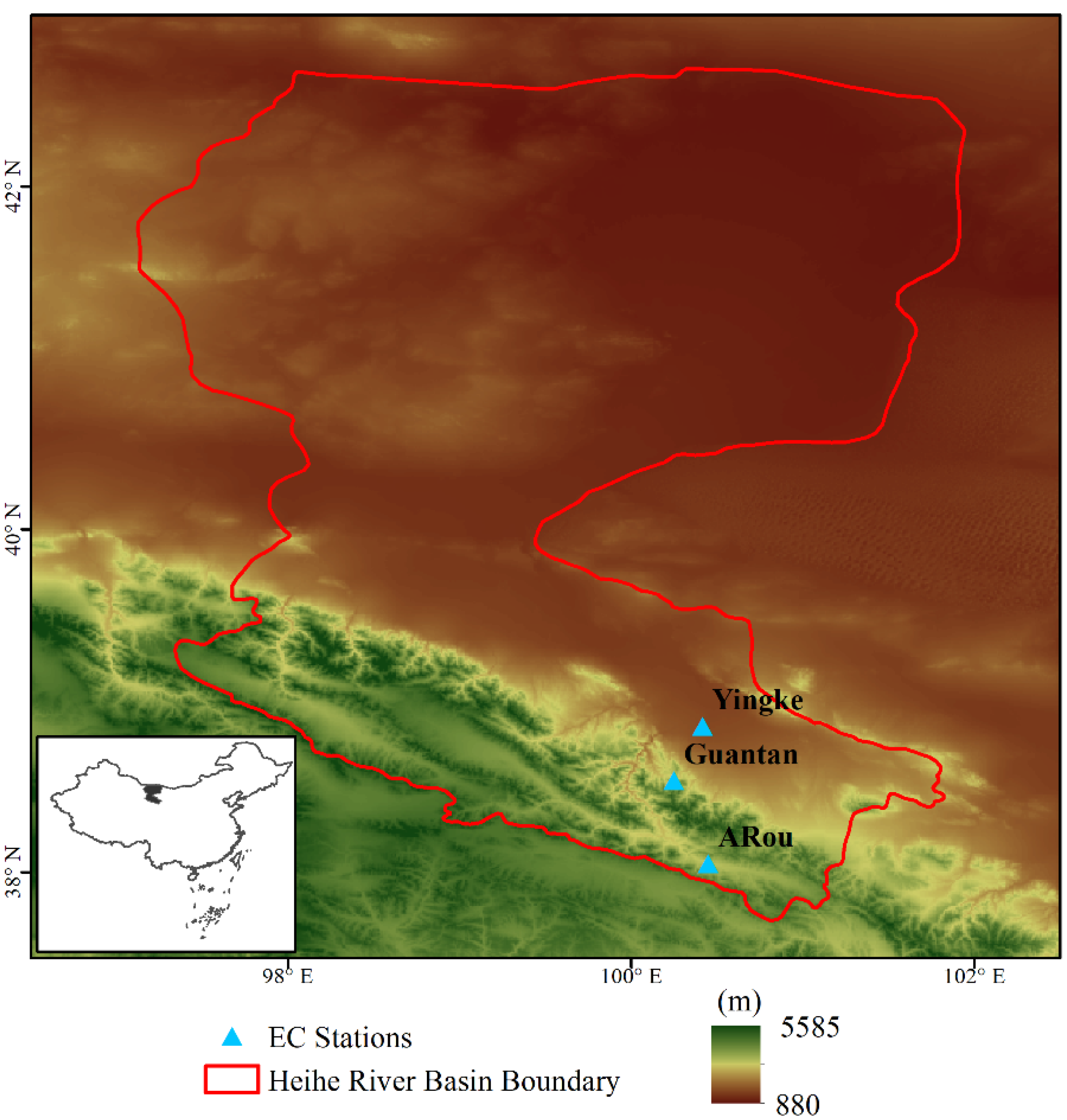
2.1. Study Area

Heihe River Basin, with an arid and semi-arid climate, was chosen as the study area. The Heihe River is the second inland river of China. This study area can be divided into three sub-stream areas, i.e., the upstream area, of mainly mountains covered by forest and grass with annual precipitation of 200–400 mm/year; the midstream area, with irrigated crops in three large artificial oases and with precipitation of 50–200 mm/year; and the downstream area, with the Gobi desert, covered by sparse vegetation and with precipitation of less than 50 mm/year [19]. Owing to the unique natural environment with arid and semi-arid regions coexisting and a mountain cryosphere, it can serve as an ideal area for studying the ET of complex ecosystems in arid and semi-arid regions. Moreover, the Heihe River Basin is equipped with good research facilities and rich datasets including hydrological–ecological–atmospheric forcing variables, vegetation–soil parameters and ET observations; many researchers use it for case studies [3,20].

2.2. Data Sets

All data sets used in this study are summarized in Table 1.

2.2.1. Input Data for DNN

The input data include satellite data and meteorological datasets, which were also the input variables for the DNN downscaling model. These input variables were selected according to the widely used Penman–Menteith equation, which describes in detail the key control factors of ET. The input data should have high spatiotemporal resolution (0.01°, daily) and were selected according to the Penman–Monteith equation, allowing it to describe the ET in theory. The satellite data were used to describe the soil–vegetation state, and the meteorological data were used to describe the environment of the soil–vegetation.

Satellite Data

Moderate Resolution Imaging Spectroradiometer (MODIS) NDVI (MOD13A2) data with a spatiotemporal resolution of 1 km and 16 days was collected from the National Aeronautics and Space Administration (NASA).
Global LAnd Surface Satellite (GLASS) gap-free Albedo data with a resolution of 1 km and 8 days were provided by Beijing Normal University. These data were retrieved from MODIS data using an angular bin algorithm and a statistics-based temporal filtering method [21].
The essential climate variable (ECV) combined surface soil moisture with resolution of 0.25° and daily in version V0.44 was provided by European Space Agency (ESA). It was generated by merging active microwave, passive microwave and modelled soil moisture data [22].

Meteorological Data

Meteorological forcing data, including wind speed (WS), air temperature (AT), relative humidity (RH), air pressure (AP), downward short-wave radiation (DSR) and downward long-wave radiation (DLR), with a resolution of 0.1° and 3 h were provided by Institute of Tibetan Plateau Research, Chinese Academy of Sciences [23]. Station data from the China Meteorological Administration (CMA), GEWEX-SRB radiation, and GLDAS data were used to enhance the quality of this dataset.

2.2.2. GLEAM ET Product

ET from the GLEAM model developed in 2011 was used in this study [24]. GLEAM ET is the total ET of soil evaporation, vegetation transpiration and rainfall interception. The spatiotemporal resolution of the GLEAM ET is 0.25° and 1 day. The main advantage of the GLEAM ET is that it considers the root zone soil moisture in the parameterization of the resistance of Priestley–Taylor equations, which enhances the model’s mechanism. The data assimilation was used to correct the error in the simulated soil moisture.

2.2.3. Ground Data

ET estimates were validated using ground data from three eddy covariance (EC) stations (Figure 1) from 2009–2011 [19,25], including one grassland EC station (Arou (AR), 3.2 m) and one forest EC station (Guantan (GT), 20.02 m) in the upper stream of the Heihe River, and one crop EC station (Yingke (YK), 2.81 m) in the middle stream. These data were downloaded from the National Tibetan Plateau Data Center. All ground data have a temporal resolution of 30 min, and were averaged to daily for this study. These three ground datasets with long-term observations representing three typical vegetation types can give an overall performance of the proposed method.

2.3. Methods

The proposed ET downscaling algorithm includes four main steps (Figure 2): (1) obtaining high spatiotemporal resolution input data; (2) obtaining low spatial resolution input data; (3) training the DNN using GLEAM ET and input data at low spatial resolution; (4) downscaling the ET to high spatial resolution using the trained DNN and high spatiotemporal resolution input data. The core process of this algorithm is training the DNN using GLEAM ET at low spatial resolution. DNN has more layers than a traditional neural network [16], which provides a strong advantage in automatically extracting complicated information from the input (input data) and is not sensitive to outliers.

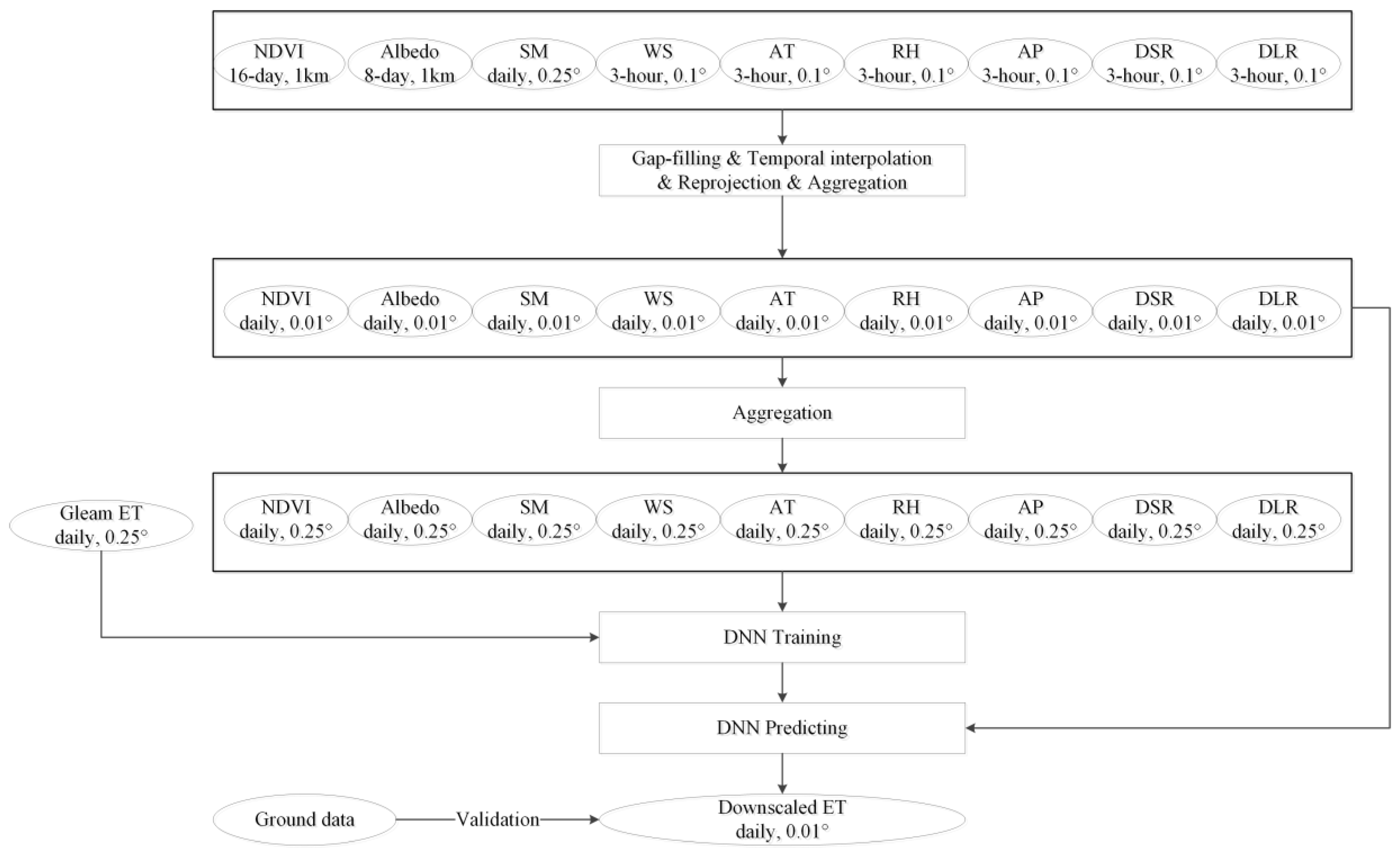
2.3.1. Obtaining High Spatiotemporal Resolution Input Data

Since the purpose of this study is to obtain high spatiotemporal resolution ET by downscaling the global ET product, we first obtained high spatial resolution (0.01°) gap-filled input data. For NDVI, there are a lot of cloud-related gaps in the time series that needed to be filled [26]. In this study, we used harmonic analysis of time series (HANTS) [27], a two-step Fourier-transform method developed for time series with irregularly spaced observations [28], to obtain gap-filled NDVI [26]. For albedo and gap-free NDVI, the bilinear interpolation method was used to improve the temporal resolution from 8 days to 1 day [29].
Meteorological data were averaged from 3 hourly to daily. For daily air temperature, air pressure, specific humidity, air pressure, longwave radiation, and shortwave radiation, the spatial resolution was improved from 0.1° to 0.01° using statistical downscaling approaches as described by [16]. For wind speed, the bilinear interpolation method was used to improve the spatial resolution from 0.1° to 0.01°.
Finally, input data with a high spatiotemporal resolution of 0.01° and 1 day (including NDVI, albedo, WS, AT, RH, AP, DSR, DLR and SM) were used as input for the DNN downscaling algorithm.

2.3.2. Obtaining Low Spatial Resolution Input Data

For the downscaling algorithm, DNN should first be trained at low spatial resolution. Hence, the input data should be processed to low resolution. Daily high spatial resolution input data of 0.01° were aggregated to low spatial resolution of 0.25°.

2.3.3. Training DNN at Low Spatial Resolution

Artificial neural network (ANN) techniques are first used to represent the high-dimension relationship between the input and the predicted variables. The concept of ANN was first proposed in 1943, and has rapidly developed in the next several decades. Compared with the early version of the ANN models, such as shallow neural networks (SNNs), the recently developed DNN contains more hidden layers within the neural network, and could better represent the features between the input and predicted variables. The network of DNN is sufficiently large that it can easily handle a large number of training data. In addition, the global training strategy can be adopted to reduce its sensitive to the outliers and show good performance. Similar to other machine learning methods, the core idea of DNN is to also establish a stable nonlinear function between input variables (input data) and predicted variable (here is ET) on a daily scale:
ET = DNN (NDVI, albedo, WS, AT, RH, AP, DLR, DSR, SM)
In this study, a four-layer DNN (9–128-128–1) was adopted. The most important parameters in DNN are the learning rate (referring to the magnitude of updating the network weight in DNN optimization), cost function (measuring the difference between the predicted and the labeled results), optimizer (improving computational efficiency) and the activation function (adding some nonlinear factors to better solve more complex problems). These important configurations adopted in the DNN model followed the previous studies [16,30,31], including a max number of echoes of 1000, linearly decreasing the learning rate of 0.9 times every 200 echoes with an initial value of 0.005, using of ‘RMSE’ and ‘Adam’ as the cost function and optimizer (Kingma and Ba, 2014; Nair and Hinton, 2010), and using the ‘ReLu’ activation function for each hidden layers. To maximize the advantages of DNN data mining, the global training strategy was adopted in this study. The training data set was divided into three parts (60:20:20) for training, validation and testing.

2.3.4. Downscaling the ET to High Spatial Resolution

In the last step, the trained DNN was driven by the high spatiotemporal resolution input data to generate daily high spatial resolution ET at 0.01°. As the input data for DNN were gap-filled at a daily scale, ET was also downscaled at daily temporal resolution.

2.3.5. Performance Metrics

Three metrics included correlation coefficient (R), the root mean squared error (RMSE), bias and Nash–Sutcliffe efficiency coefficient (NSE) were used to validate the downscaled ET:
r = i = 1 N ( E T m i E T m ¯ ) ( E T o i E T o ¯ ) i = 1 N ( E T m i E T m ¯ ) 2 i = 1 N ( E T o i E T o ¯ ) 2
R M S E = 1 N i = 1 N ( E T m i E T o i ) 2
b i a s = 1 N i = 1 N ( E T m i E T o i )
N S R = 1 i = 1 N ( E T 0 i E T m i ) 2 i = 1 N ( E T 0 i E T o ¯ ) 2
where E T m i and E T o i are the i-th estimated and observed or original ET, respectively; E T m ¯ is the average of the estimated ET, E T o ¯ is the average of the observed or original ET and N is the number of observations.

3. Results

The main objective of this study is to obtain high spatial resolution ET by downscaling the global ET products. Hence, three aspects were designed to assess the methods: (1) validation the original and downscaled ET against the in situ observations; (2) showing the consistency of the downscaled ET and the original product; (3) analyzing the importance of the input variables. It is worth mentioning that analyzing the original ET can be considered as a comparison with statistical downscaling method (i.e., the Nearest neighbor sampling method).

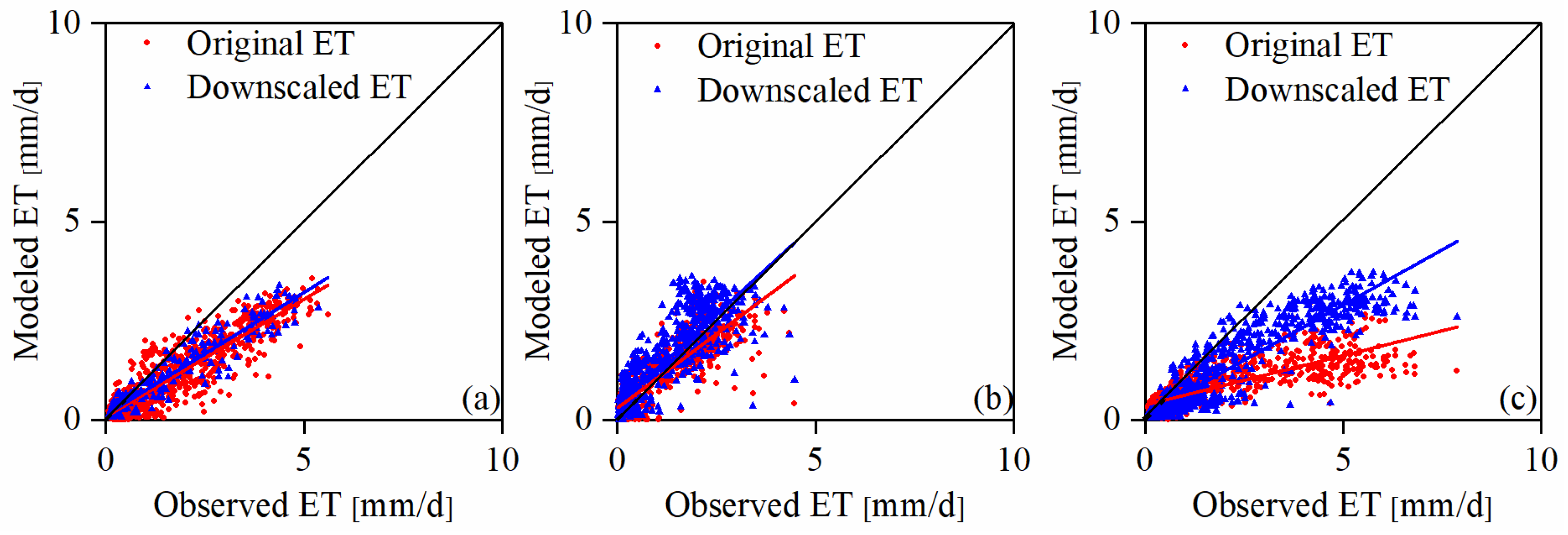
3.1. Overall Performance of the Original and Downscaled ET

We used satellite and meteorological data with high spatiotemporal resolution to downscale GLEAM ET using the DNN. In the training phase of the DNN, there are about 100,000 samples used to train the DNN. The overall R and RMSE were about 0.9 and 0.5 mm/d, showing good performance of the proposed scheme. To further assess the overall performance of the proposed method, the downscaled and original GLEAM global ET were compared against in situ observations at YK, AR and GT stations in the Heihe River Basin and the results are shown in Figure 3 and Table 2.
For the original GLEAM ET, the overall R and RMSE (bias) is 0.85 and 1.08 mm/d (−0.55 mm/d), respectively, showing acceptable accuracy. The GLEAM ET at AR station had the best performance, while the worst performance was at the YK station. This is because the YK station is located in the irrigated cropland where there are about five irrigation events, which make it difficult to simulate ET by the GLEAM model at low spatial resolution. Because of the lacks of irrigation information, the GLEAM model did not capture its effect on ET. Another reason is that the spatial heterogeneity of the surrounding environment is stronger at YK than at the AR and GT stations. In this situation, the coarse resolution of the ET product showed a strong disadvantage.
For the downscaled ET, the overall R and RMSE (bias, NSR) was 0.90 and 0.87 mm/d (−0.32 mm/d, 0.62), respectively. Compared with the original GLEAM ET, the R of downscaled ET was improved by about 5.9%, RMSE was improved by 19.4% and NSR was improved by 40.9%. The most significant improvement was found at YK station, with improved R and RMSE (NSR) of 17.9% and 33.3% (5700%), respectively. The main reason for this is that the GLEAM ET is highly dependent on the simulated surface and root zone soil moisture with the water balance, which is unbalanced over the irrigated YK station due to lack of irrigation information [3,32]. Consequently, the DNN with global training strategy has greater advantage than the traditional machine learning method, which always has to adopt a moving window strategy to deal with a large number of training data. Another reason might be because the downscaled ET reduced the mismatch between the pixel and the footprint of the EC observations, which is always less than 1 km, indicating that spatially downscaling the global ET product is necessary for the most end users. It is worth noting that this reduced mismatch does not always result in better performance under high resolution for the complex surface, such as the pixels of the original GLEAM ET at the GT station, which were covered by vastly different types of forest and grassland.

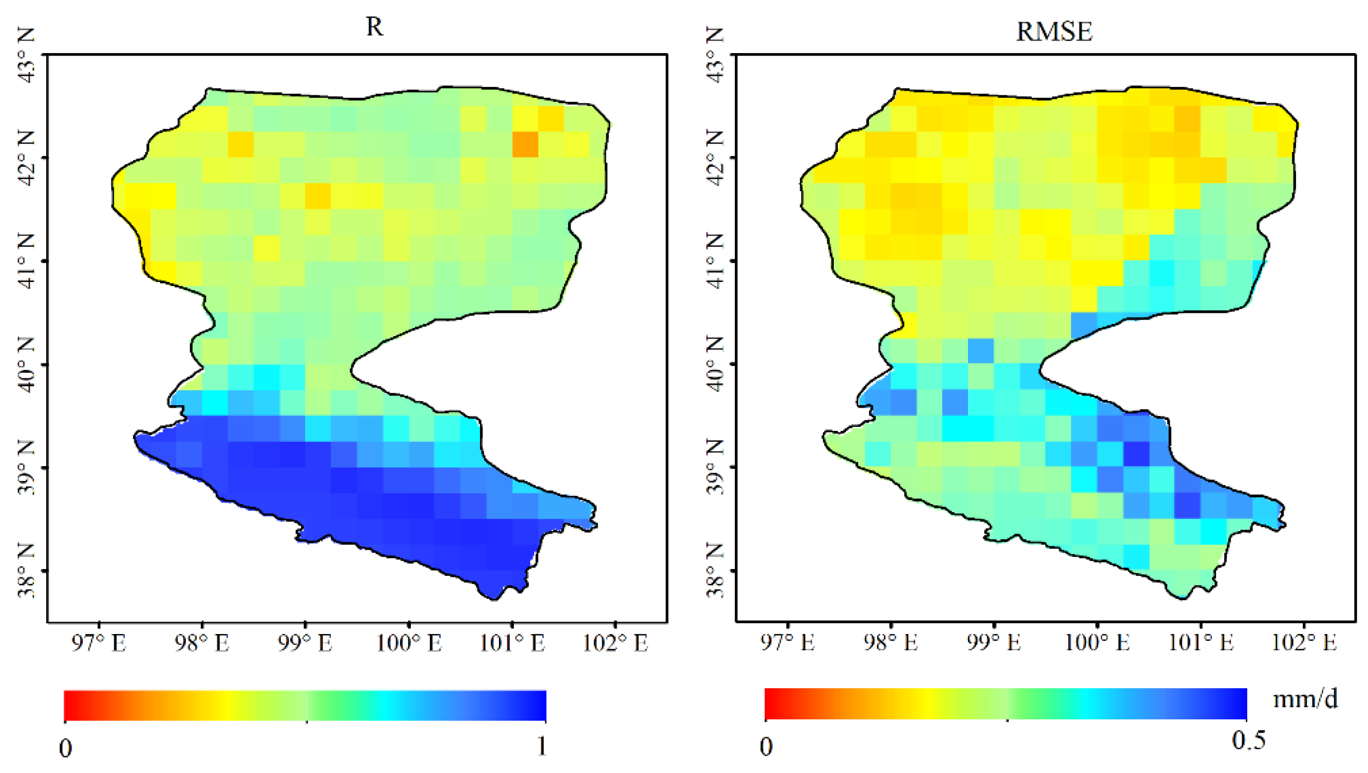
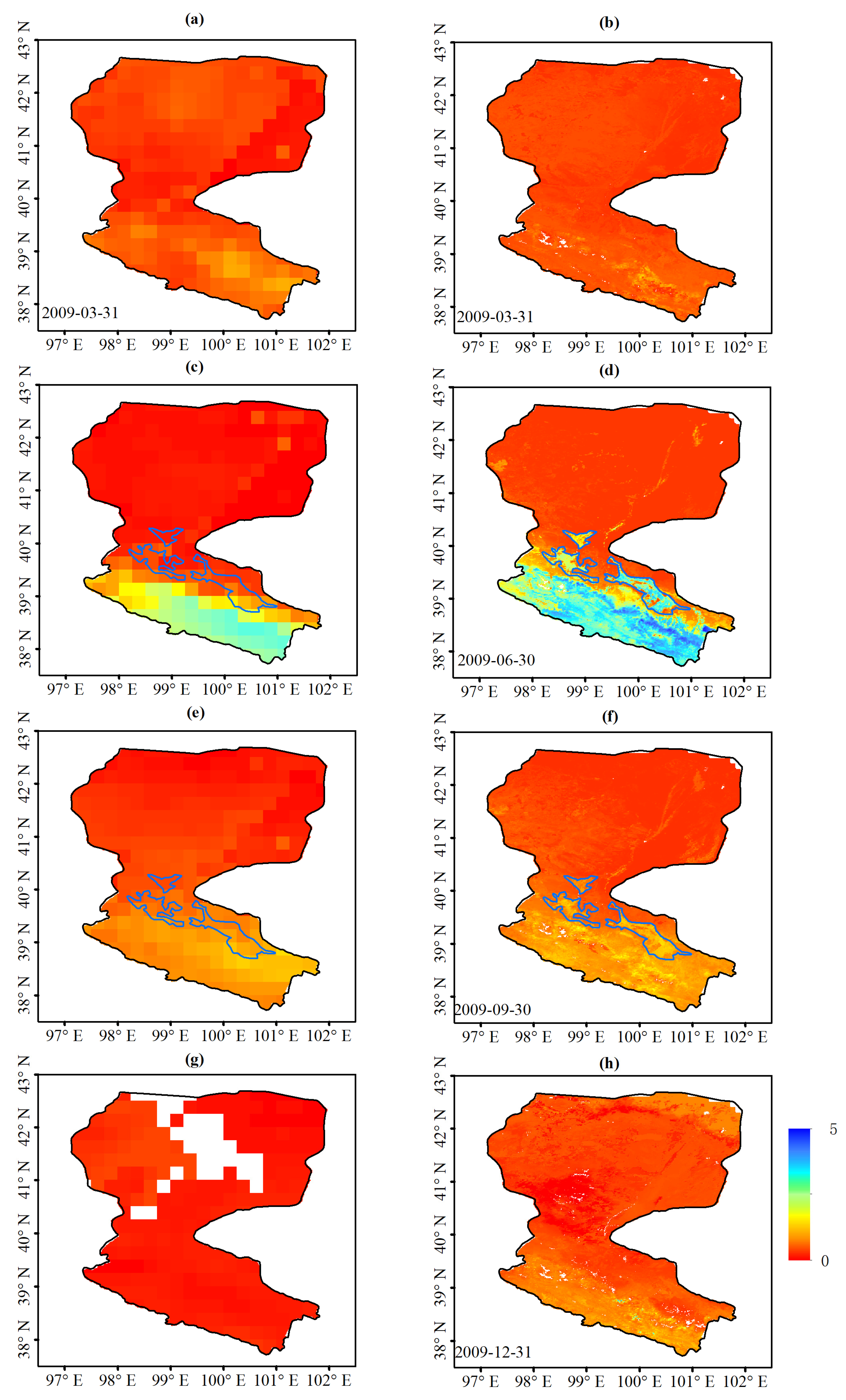
3.2. Spatial and Temporal Comparison of the Downscaled and Original ET

Figure 4 shows the spatial patterns of the original and downscaled ET in different seasons, indicating a generally consistent pattern at the regional scale. Both ET datasets decrease from south to north, reflecting regional limits in available water. Temporal variability is also very similar in the original and downscaled ET, where high in summer and low in the other seasons. These patterns indicate that the DNN can capture the temporal variability of the original ET products.
The main difference between the both datasets is the greater detailed information being shown by the downscaled ET. This indicates that the DNN performs well at downscaling the global ET.
The relatively higher ET over the irrigated oasis (enclosed area) than over the surrounding desert is much clearer in the downscaled ET map than in the original ET map. This indicates that the DNN performs well, even where the land surface presents strong heterogeneity.
To further understand the similarity and difference between the original and downscaled ET, the R and RMSE between them was calculated at 0.25° resolution, after averaging the downscaled ET map from 0.01° to 0.25° (Figure 5). The R is higher in the upstream area (R > 0.9), while lower in the mid- and downstream areas, indicating that the DNN mainly captured the features from the upstream training data. This is because the downstream area is covered by a huge desert with very small ET, and the lower variability in the input data makes it difficult to reach stability in the training of the DNN. This difference indicates a large scope for improving the DNN in complex regions such as the study area. The RMSE is lower than 0.5 mm/d showing high training accuracy. The lower R area has also a lower RMSE, indicating the reliability of the DNN.

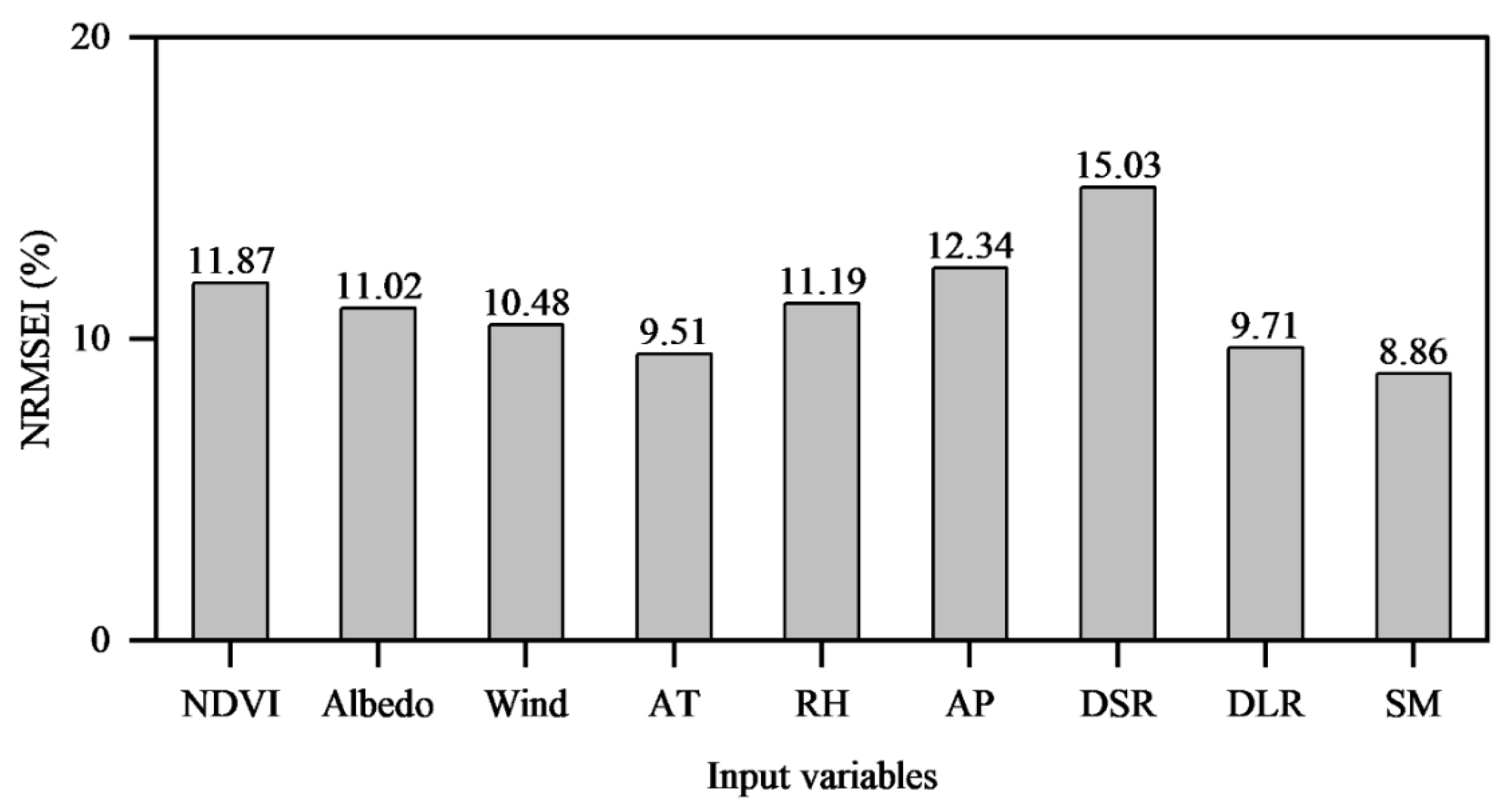
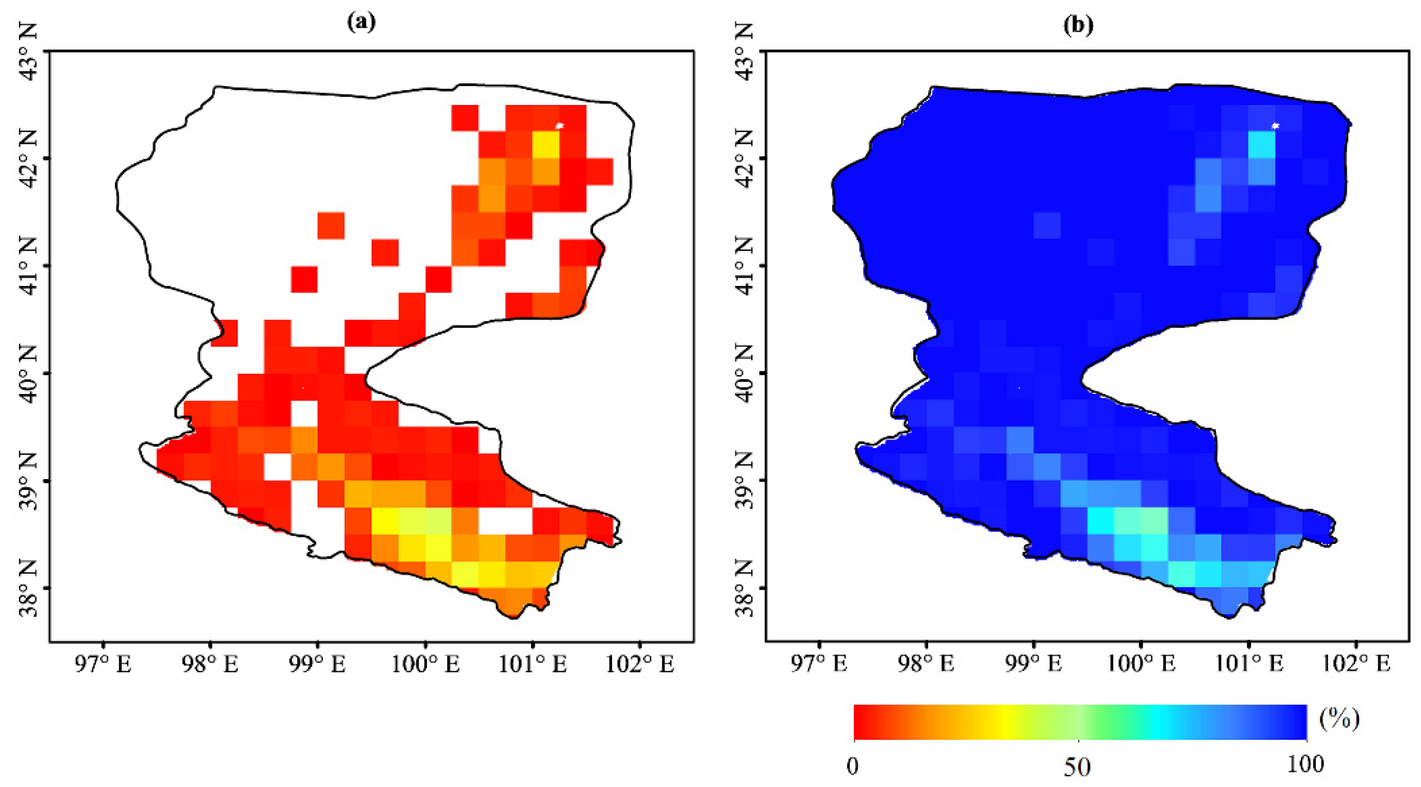
3.3. Analyzing Importance of Input Variables

With the help of the high spatiotemporal input datasets (input variables for the DNN), the DNN model was successfully used to improve the spatial resolution of the GLEAM ET product. However, the downscaled ET is not only limited by the quality of the original ET product, but also limited by the input variables. Hence, it is necessary to analyze the importance of different input variables to understand the importance of the variables to the DNN model for ET downscaling. An index named the normal root mean square error index (NRMSEI) was used to quantitatively describe this importance, which is the normalized RMSE between the downscaled ET from the DNN model when one variable is not included against when all variables are included. The larger NRMSEI, the more important the variable is to the downscaled ET. The NRMSEI is shown in Figure 6. The DSR (15.03%) plays the most important role, which is related to the surface energy balance, followed by the AP (12.34%) related to the complex terrain and NDVI (11.87%) related to the vegetation growth. The more important variables, the higher the quality requirements of the input dataset. Wind speed (10.48%) data are always considered to have a relatively larger error but moderate importance. All of the variables seem comparable in importance. The SM showed the least importance (8.86%), but it is worth mentioning that SM is still cannot be removed from the input dataset. Otherwise, it will result into more than 0.15 mm/d uncertainty.

4. Discussion

4.1. The Effect of Land Cover

Generally, the land cover has a strong effect on ET modeling due to the different canopy structure and the evapotranspiration mechanism of tall vegetation (e.g., forest) and low vegetation (e.g., grassland/cropland), according to the Penman–Monteith equation [33]. However, the land surface always presents strong heterogeneity, making it difficult to obtain pure pixels for all types of vegetation at the 0.25° resolution of GLEAM. For example, the maximum ratio of tall vegetation in the study area is lower than 50% (Figure 7). Hence, it is difficult to build two separate models to downscale the tall vegetation and the low vegetation, separately. For this reason, this study did not consider land cover. This will result a lower ratio for the tall vegetation with, which has limited information in the training phase of the DNN and introduces large uncertainty in the downscaling process. In the future, considering the land cover in the downscaling process is a direction to further improve the performance of this method.

4.2. Advantages and Limitations of This Study

The DNN model, combined with the input data from remote sensing and meteorology, was successfully applied to produce high spatiotemporal resolution ET in an arid and semi-arid area. The downscaled ET was consistent with the original ET in spatial pattern and temporal variability. Against the in situ observations, the downscaled ET is a good reflection of the temporal variability of the original product. The DNN showed a good performance, despite the huge heterogeneity in the land surface. Meanwhile, the proposed method can generate the daily ET, which has higher temporal resolution than the widely used MODIS ET product with 8 days. We further compared the downscaled ET estimates against the MODIS ET product (Table 3). To make the results comparable, we resampled the downscaled GLEAM ET from 1 day to 8 days. Against the in situ measurements, the downscaled ET has higher accuracy than the MODIS product with overall R (RMSE, bias, NSE) of 0.94 (0.76 mm d−1, −0.31 mm d−1, 0.67) vs. 0.84 (0.82 mm d−1, −0.5 mm d−1, 0.6), showing that the DNN is an accessible tool to obtain high resolution ET product from the global products.
However, because the original ET was, on the whole, underestimated, the downscaled ET also underestimated the ET. Hence, simultaneously improving the spatial resolution and quality of the ET product is a challenging task, but should be considered in the future because of its relevance for the end user. Field-scale ET estimates (e.g., 30 m) of agricultural land can better meet the needs of precision management of water resources. In future work, we will obtain field-scale input data to derive field-scale ET estimates.

5. Conclusions

Based on the DNN model, basin-wide high spatiotemporal resolution ET (daily, 0.01°) was obtained by combining the GLEAM ET, remotely sensed data (NDVI, Albedo and SM) and meteorological data (wind speed, air temperature, relative humidity, air pressure, downward shortwave radiation, and downward longwave radiation). Major conclusions are given below. The downscaled GLEAM ET shows a consistent spatial pattern with the original ET product, but shows more detailed information on the spatiotemporal variability of ET. Compared with the in situ ET observations, the downscaled GLEAM ET can effectively reflect the quality in the study area. Major conclusions are given as follows.
(1)
The overall R, RMSE, bias and NSE between the downscaled ET and the ground ET are 0.90, 0.87 mm/d, −0.32 mm/d and 0.62, respectively, which are better than the original ET with overall R, RMSE, bias and NSE of 0.85, 1.08 mm/d, −0.55 mm/d and 0.44, respectively.
(2)
The downscaled ET is highly consistent with the original ET, especially for the temporal variability. However, quality of the downscaled ET is strongly affected by the original product.
In summary, this study successfully downscaled the coarse resolution ET of 0.25° to high resolution of 0.01°, meeting the requirement of end users. In the future, simultaneously improving quality and spatial resolution at field-scale (30 m) will be discussed.

Author Contributions

Conceptualization, methodology, analysis, software, validation and visualization, X.L. and Y.C.; writing—original draft preparation, X.L.; writing—review and editing, Y.C. All authors have read and agreed to the published version of the manuscript.

Funding

This study was financially supported by the National Natural Science Foundation of China (Grant No. 41901348), Chinese Academy of Sciences-People’s Government of Qinghai Province on Sanjiangyuan National Park (LHZX-2020-10) and Scientific and Technological Research Program of Chongqing Municipal Education Commission (GrantNo.KJZD-K202100201).

Institutional Review Board Statement

Not applicable.

Informed Consent Statement

Not applicable.

Data Availability Statement

The GLEAM ET data are publicly available at the website: https://www.gleam.eu/. The MODIS data are publicly available at the website https://modis.gsfc.nasa.gov/. The GLASS data are publicly available at the website http://www.glass.umd.edu/. The ECV SM data are publicly available at the website: https://www.esa-soilmoisture-cci.org/. The CMFD Meteorological data and in situ validation data are publicly available at the website: http://data.tpdc.ac.cn/en/.

Acknowledgments

The authors thank two anonymous reviewers for their valuable comments.

Conflicts of Interest

The authors declare no conflict of interest.

References

  1. Kim, S.H.; Sicher, R.C.; Bae, H.; Gitz, D.C.; Reddy, V.R.J.G.C.B. Canopy photosynthesis, evapotranspiration, leaf nitrogen, and transcription profiles of maize in response to CO2 enrichment. Glob. Chang. Biol. 2010, 12, 588–600. [Google Scholar] [CrossRef]
  2. Cui, Y.; Chen, X.; Gao, J.; Yan, B.; Tang, G.; Hong, Y. Global water cycle and remote sensing big data: Overview, challenge, and opportunities. Big Earth Data 2018, 2, 282–297. [Google Scholar] [CrossRef]
  3. Cui, Y.; Jia, L. Estimation of evapotranspiration of “soil-vegetation” system with a scheme combining a dual-source model and satellite data assimilation. J. Hydrol. 2021, 603, 127145. [Google Scholar] [CrossRef]
  4. Li, S.; Kang, S.; Zhang, L.; Ortega-Farias, S.; Li, F.; Du, T.; Tong, L.; Wang, S.; Ingman, M.; Guo, W. Measuring and modeling maize evapotranspiration under plastic film-mulching condition. J. Hydrol. 2013, 503, 153–168. [Google Scholar] [CrossRef]
  5. Mu, Q.; Zhao, M.; Kimball, J.S.; McDowell, N.G.; Running, S.W. A remotely sensed global terrestrial drought severity index. Bull. Am. Meteorol. Soc. 2013, 94, 83–98. [Google Scholar] [CrossRef] [Green Version]
  6. Cui, Y.; Jia, L.; Fan, W. Estimation of actual evapotranspiration and its components in an irrigated area by integrating the Shuttleworth-Wallace and surface temperature-vegetation index schemes using the particle swarm optimization algorithm. Agric. For. Meteorol. 2021, 307, 108488. [Google Scholar] [CrossRef]
  7. Wang, K.C.; Dickinson, R.E. A review of global terrestrial evapotranspiration: Observation, modeling, climatology, and climatic variability. Rev. Geophys. 2012, 50, 373. [Google Scholar] [CrossRef]
  8. Zhang, K.; Kimball, J.S.; Running, S.W. A review of remote sensing based actual evapotranspiration estimation. Wiley Interdiscip. Rev. Water 2016, 3, 834–853. [Google Scholar] [CrossRef]
  9. Rodell, M.; Houser, P.R.; Jambor, U.; Gottschalck, J.; Mitchell, K.; Meng, C.J.; Arsenault, K.; Cosgrove, B.; Radakovich, J.; Bosilovich, M.; et al. The global land data assimilation system. Bull. Am. Meteorol. Soc. 2004, 85, 381–394. [Google Scholar] [CrossRef] [Green Version]
  10. Martens, B.; Miralles, D.G.; Lievens, H.; van der Schalie, R.; de Jeu, R.A.M.; Fernández-Prieto, D.; Beck, H.E.; Dorigo, W.A.; Verhoest, N.E.C. GLEAM v3: Satellite-based land evaporation and root-zone soil moisture. Geosci. Model Dev. 2017, 10, 1903–1925. [Google Scholar] [CrossRef] [Green Version]
  11. Martens, B.; Miralles, D.; Lievens, H.; Fernández-Prieto, D.; Verhoest, N.E.C. Improving terrestrial evaporation estimates over continental Australia through assimilation of SMOS soil moisture. Int. J. Appl. Earth Obs. Geoinf. 2016, 48, 146–162. [Google Scholar] [CrossRef]
  12. Mu, Q.Z.; Zhao, M.S.; Running, S.W. Improvements to a MODIS global terrestrial evapotranspiration algorithm. Remote Sens. Environ. 2011, 115, 1781–1800. [Google Scholar] [CrossRef]
  13. Cui, Y.; Chen, X.; Xiong, W.; He, L.; Lv, F.; Fan, W.; Luo, Z.; Hong, Y. A Soil Moisture Spatial and Temporal Resolution Improving Algorithm Based on Multi-Source Remote Sensing Data and GRNN Model. Remote Sens. 2020, 12, 455. [Google Scholar] [CrossRef] [Green Version]
  14. Zhao, W.; Sánchez, N.; Lu, H.; Li, A. A spatial downscaling approach for the SMAP passive surface soil moisture product using random forest regression. J. Hydrol. 2018, 563, 1009–1024. [Google Scholar] [CrossRef]
  15. Nanjundiah, S. Downscaling of precipitation for climate change scenarios: A support vector machine approach. J. Hydrol. 2006, 330, 621–640. [Google Scholar]
  16. Cui, Y.; Song, L.; Fan, W. Generation of spatio-temporally continuous evapotranspiration and its components by coupling a two-source energy balance model and a deep neural network over the Heihe River Basin. J. Hydrol. 2021, 597, 126176. [Google Scholar] [CrossRef]
  17. Tran Anh, D.; Van, S.P.; Dang, T.D.; Hoang, L.P. Downscaling rainfall using deep learning long short-term memory and feedforward neural network. Int. J. Climatol. 2019, 39, 4170–4188. [Google Scholar] [CrossRef]
  18. Xu, W.; Zhang, Z.; Long, Z.; Qin, Q. Downscaling SMAP Soil Moisture Products with Convolutional Neural Network. IEEE J. Sel. Top. Appl. Earth Obs. Remote Sens. 2021, 14, 4051–4062. [Google Scholar] [CrossRef]
  19. Li, X.; Li, X.W.; Li, Z.Y.; Ma, M.G.; Wang, J.; Xiao, Q.; Liu, Q.; Che, T.; Chen, E.X.; Yan, G.J.; et al. Watershed Allied Telemetry Experimental Research. J. Geophys. Res. Atmos. 2009, 114, 11590. [Google Scholar] [CrossRef] [Green Version]
  20. Hu, G.; Jia, L. Monitoring of Evapotranspiration in a Semi-Arid Inland River Basin by Combining Microwave and Optical Remote Sensing Observations. Remote Sens. 2015, 7, 3056–3087. [Google Scholar] [CrossRef] [Green Version]
  21. Liu, N.; Liu, Q.; Wang, L.; Wen, J. A temporal filtering algorithm to reconstruct daily albedo series based on GLASS albedo product. In Proceedings of the Geoscience and Remote Sensing Symposium (IGARSS), Vancouver, BC, Canada, 24–29 July 2011; pp. 4277–4280. [Google Scholar]
  22. Liu, Y.Y.; Parinussa, R.M.; Dorigo, W.A.; de Jeu, R.A.M.; Wagner, W.; van Dijk, A.I.J.M.; McCabe, M.F.; Evans, J.P. Developing an improved soil moisture dataset by blending passive and active microwave satellite-based retrievals. Hydrol. Earth Syst. Sci. 2011, 15, 425. [Google Scholar] [CrossRef] [Green Version]
  23. He, J.; Yang, K.; Tang, W.; Lu, H.; Qin, J.; Chen, Y.; Li, X. The first high-resolution meteorological forcing dataset for land process studies over China. Sci. Data 2020, 7, 25. [Google Scholar] [CrossRef] [PubMed] [Green Version]
  24. Miralles, D.G.; Holmes, T.R.H.; De Jeu, R.A.M.; Gash, J.H.; Meesters, A.G.C.A.; Dolman, A.J. Global land-surface evaporation estimated from satellite-based observations. Hydrol. Earth Syst. Sci. 2011, 15, 453–469. [Google Scholar] [CrossRef] [Green Version]
  25. Liu, S.; Li, X.; Xu, Z.; Che, T.; Xiao, Q.; Ma, M.; Liu, Q.; Jin, R.; Guo, J.; Wang, L.; et al. The Heihe Integrated Observatory Network: A Basin-Scale Land Surface Processes Observatory in China. Vadose Zone J. 2018, 17, 180072. [Google Scholar] [CrossRef]
  26. Jia, L.; Shang, H.; Hu, G.; Menenti, M. Phenological response of vegetation to upstream river flow in the Heihe Rive basin by time series analysis of MODIS data. Hydrol. Earth Syst. Sci. 2011, 15, 1047–1064. [Google Scholar] [CrossRef] [Green Version]
  27. Menenti, M.; Azzali, S.; Verhoef, W.; Vanswol, R. Mapping Agroecological Zones And Time-Lag In Vegetation Growth by Means Of Fourier-Analysis Of Time-Series Of Ndvi Images. Adv. Space Res. 1993, 13, 233–237. [Google Scholar] [CrossRef]
  28. Jia, L.; Xi, G.; Liu, S.; Huang, C.; Yan, Y.; Liu, G. Regional estimation of daily to annual regional evapotranspiration with MODIS data in the Yellow River Delta wetland. Hydrol. Earth Syst. Sci. 2009, 13, 1775–1787. [Google Scholar] [CrossRef] [Green Version]
  29. Cui, Y.; Long, D.; Hong, Y.; Zeng, C.; Zhou, J.; Han, Z.; Liu, R.; Wan, W. Validation and reconstruction of FY-3B/MWRI soil moisture using an artificial neural network based on reconstructed MODIS optical products over the Tibetan Plateau. J. Hydrol. 2016, 543, 13. [Google Scholar] [CrossRef]
  30. Tao, Y.; Gao, X.; Hsu, K.; Sorooshian, S.; Ihler, A. A deep neural network modeling framework to reduce bias in satellite precipitation products. J. Hydrometeorol. 2016, 17, 931–945. [Google Scholar] [CrossRef]
  31. Fang, K.; Shen, C.; Kifer, D.; Xiao, Y.J.G.R.L. Prolongation of SMAP to Spatio-temporally Seamless Coverage of Continental US Using a Deep Learning Neural Network. Geophys. Res. Lett. 2017, 44, 11–30. [Google Scholar] [CrossRef] [Green Version]
  32. Cui, G.X.; Leng, H.J.; Wang, K.; Wang, J.W.; Zhu, S.N.; Jia, J.; Chen, X.; Zhang, W.G.; Qin, L.H.; Bai, W.P. Effects of Remifemin Treatment on Bone Integrity and Remodeling in Rats with Ovariectomy-Induced Osteoporosis. PLoS ONE 2013, 8, e82815. [Google Scholar] [CrossRef] [PubMed]
  33. Monteith, J.L. Evaporation and environment. Symp. Soc. Exp. Biol. 1965, 19, 205–234. [Google Scholar] [PubMed]
Figure 1. Location of Heihe River Basin and the eddy covariance (EC) stations on the digital elevation model map of the region. Guantan and ARou stations are located in the upstream, Yingke station is located in midstream.
Remotesensing 14 00658 g001
Figure 2. Flowchart of global ET downscaling algorithm based on the deep neural network (DNN). NDVI: normalized difference vegetation index; SM: soil moisture; WS: wind speed; AT: air temperature; RH: relative humidity; AP: air pressure; DSR: downward shortwave radiation; DLR: downward longwave radiation.
Remotesensing 14 00658 g002
Figure 3. Comparison of the original and downscaled ET from DNN model against in situ ET observations at AR (a), GT (b) and YK (c) stations.
Remotesensing 14 00658 g003
Figure 4. Spatial and temporal comparison of the original (left) and downscaled (right) GLEAM ET in the different seasons (on DOY = 90 (a,b), 181 (c,d), 273 (e,f), 365 (g,h) in 2009). Overlaid in blue (enclosed area) in the midstream of the Heihe River Basin is the irrigated cropland area. Unit: mm/d.
Remotesensing 14 00658 g004
Figure 5. Similarity and difference between original and downscaled ET.
Remotesensing 14 00658 g005
Figure 6. Importance of input variables (NRMSEI) of the DNN model.
Remotesensing 14 00658 g006
Figure 7. Ratio of tall vegetation (a) and low vegetation (b) at 0.25° resolution of GLEAM.
Remotesensing 14 00658 g007
Table 1. List of input data, GLEAM ET product and ground data used in this study. NDVI: normalized difference vegetation index; SM: soil moisture; WS: wind speed; AT: air temperature; RH: relative humidity; AP: air pressure; DSR: downward short-wave radiation; DLR: downward long-wave radiation; ET: evapotranspiration.
TypeVariableData SetsSpatiotemporal Resolution
Input dataNDVIMOD13A21 km/8 d
AlbedoGLASS1 km/8 d
SMESA ECV0.25°/daily
WSDAMCTM0.1°/3 h
ATDAMCTM0.1°/3 h
RHDAMCTM0.1°/3 h
APDAMCTM0.1°/3 h
DSRDAMCTM0.1°/3 h
DLRDAMCTM0.1°/3 h
GLEAMETV03.3a0.25°/daily
Ground-dataET--Point/30 min
Table 2. Comparisons of metrics of the original and downscaled GLEAM ET against in situ observations at AR, GT and YK stations.
StationsOriginal ET Downscaled ET
RRMSEBiasNSERRMSEBiasNSE
AR0.910.85−0.520.630.950.74−0.430.71
GT0.840.540.030.700.850.640.280.59
YK0.781.83−1.16−0.010.921.22−0.790.56
Mean0.851.08−0.550.440.900.87−0.320.62
Table 3. Comparison between ET estimates from this study and MODIS at AR, GT and YK stations during 2009–2011. Unit of RMSE and bias is: mm d−1.
StationsThis Study MODIS ET
RRMSEBiasNSERRMSEBiasNSE
AR0.960.67−0.400.730.850.67−0.800.67
GT0.930.450.270.740.850.520.090.68
YK0.941.17−0.800.540.831.27−0.800.45
Mean0.940.76−0.310.670.840.82−0.500.60
Publisher’s Note: MDPI stays neutral with regard to jurisdictional claims in published maps and institutional affiliations.

