
Long Term Indian Ocean Dipole (IOD) Index Prediction Used Deep Learning by convLSTM


Abstract
:1. Introduction
2. Materials and Methods
2.1. Materials
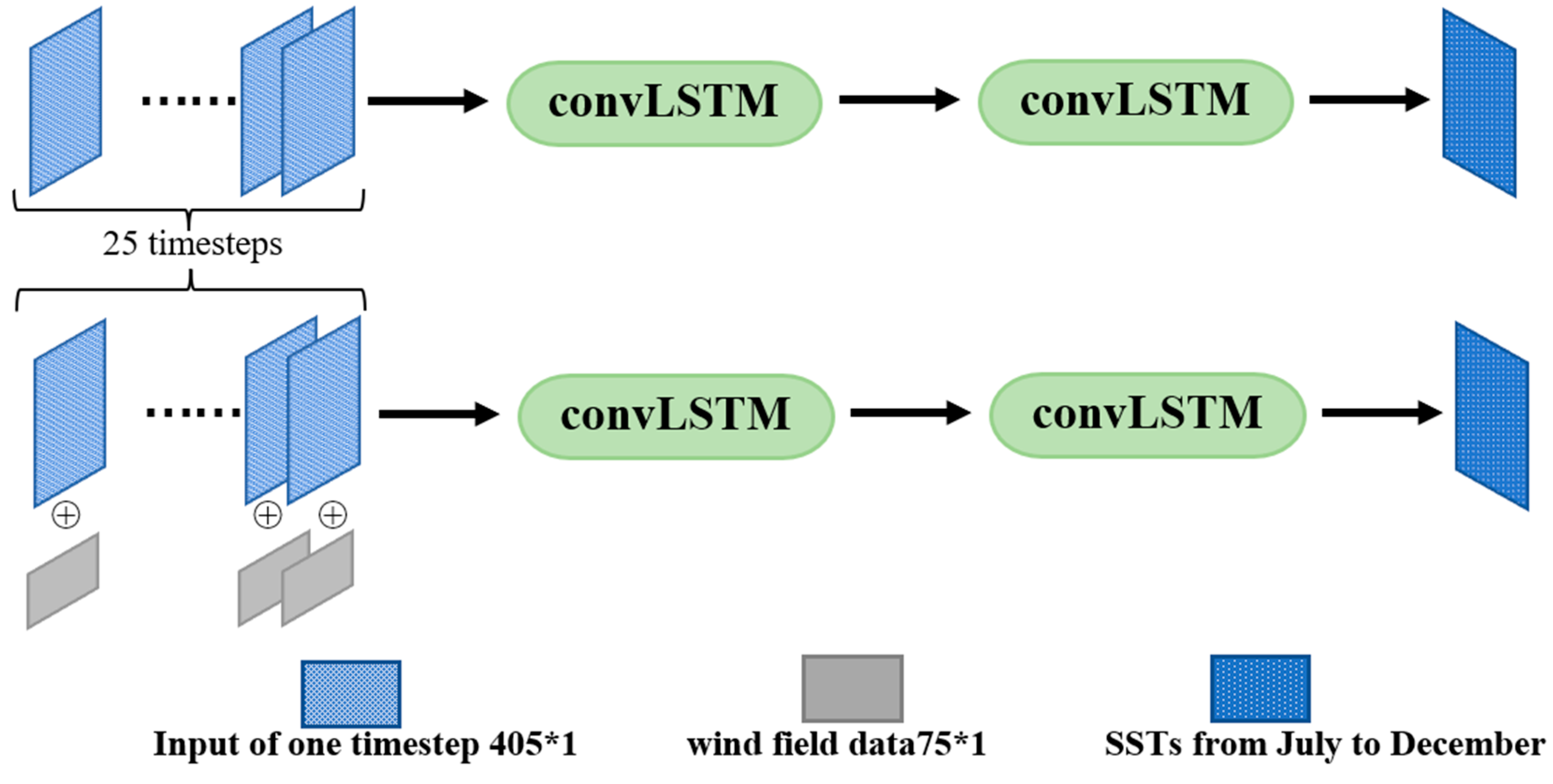
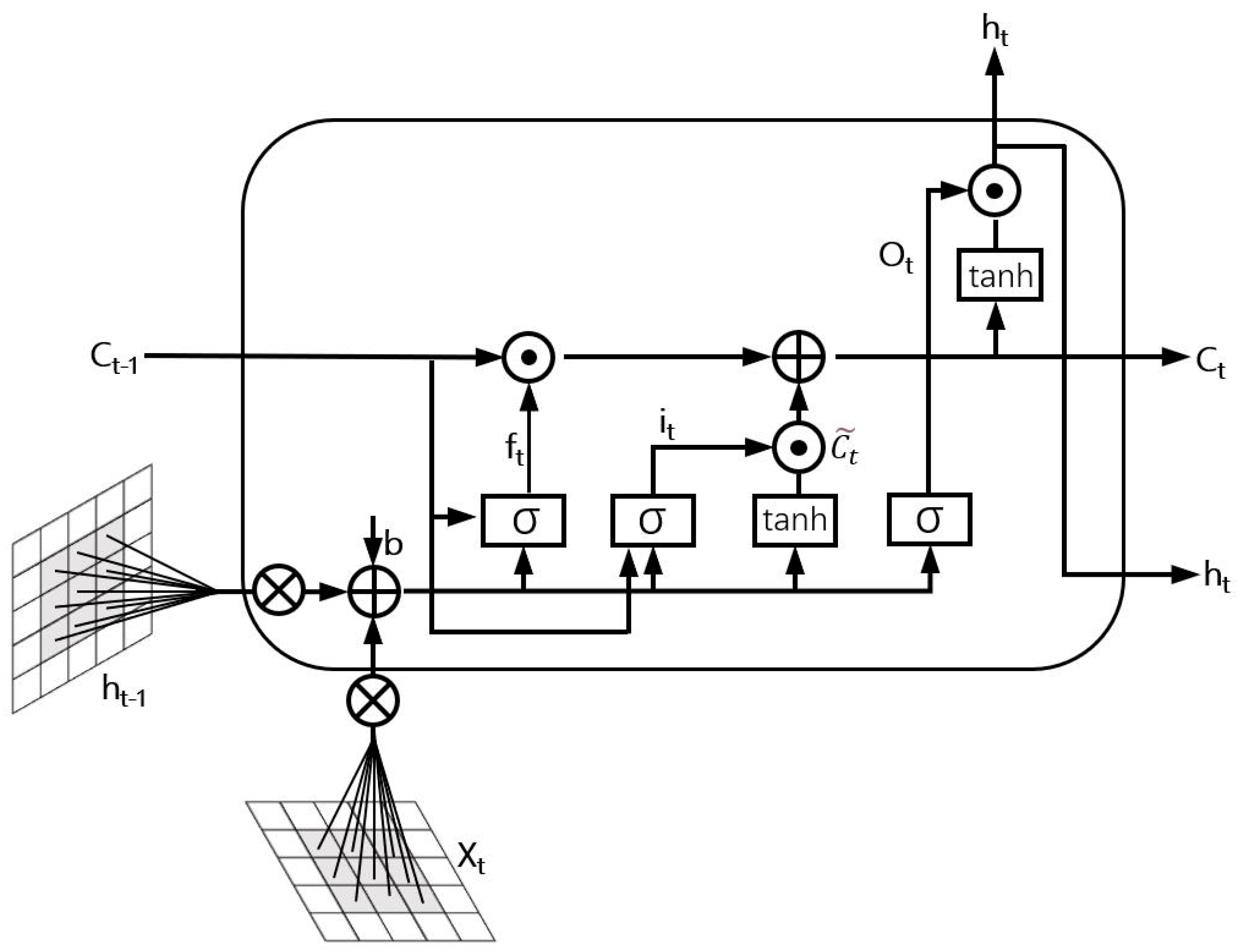
2.2. Method
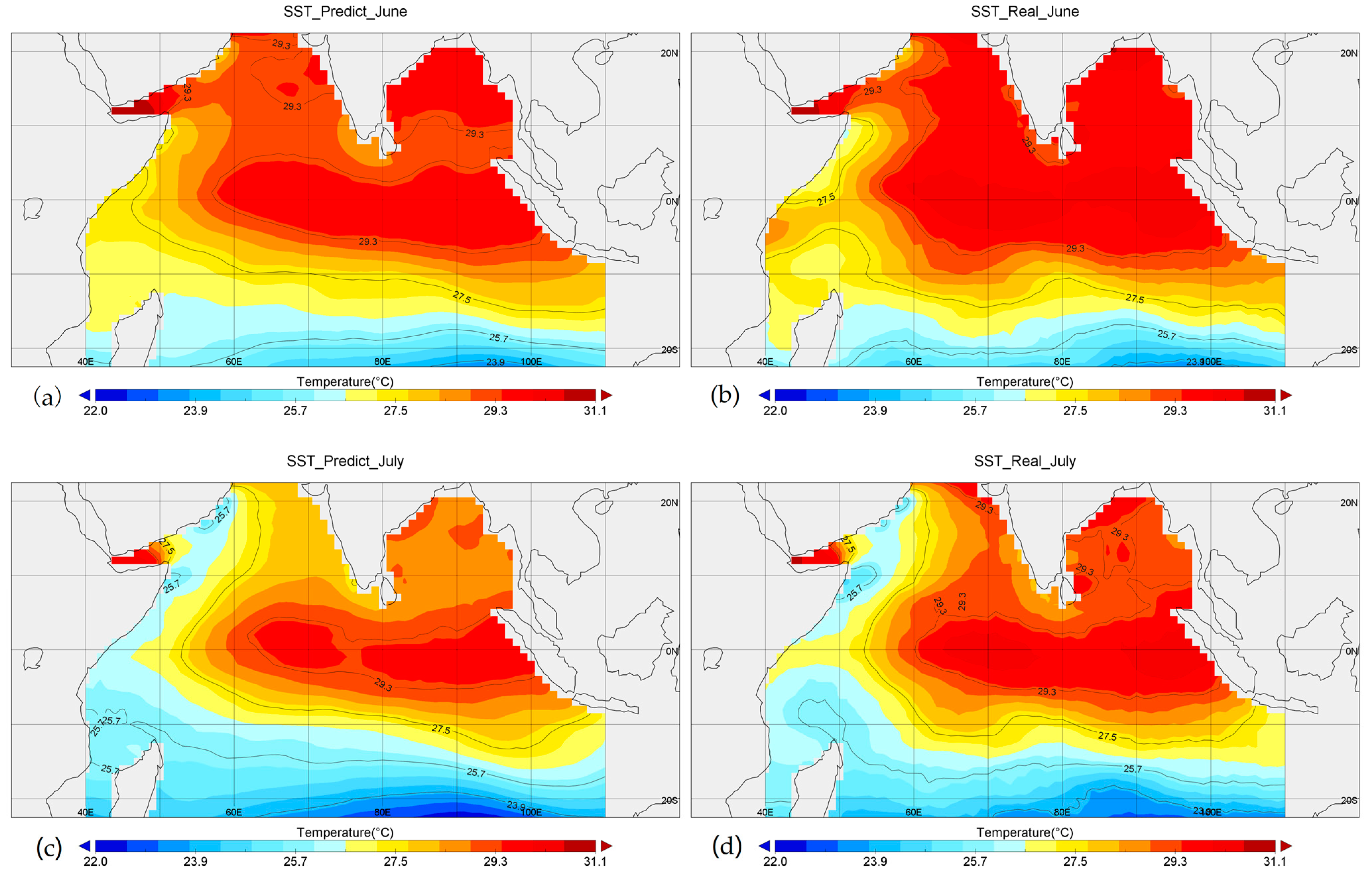
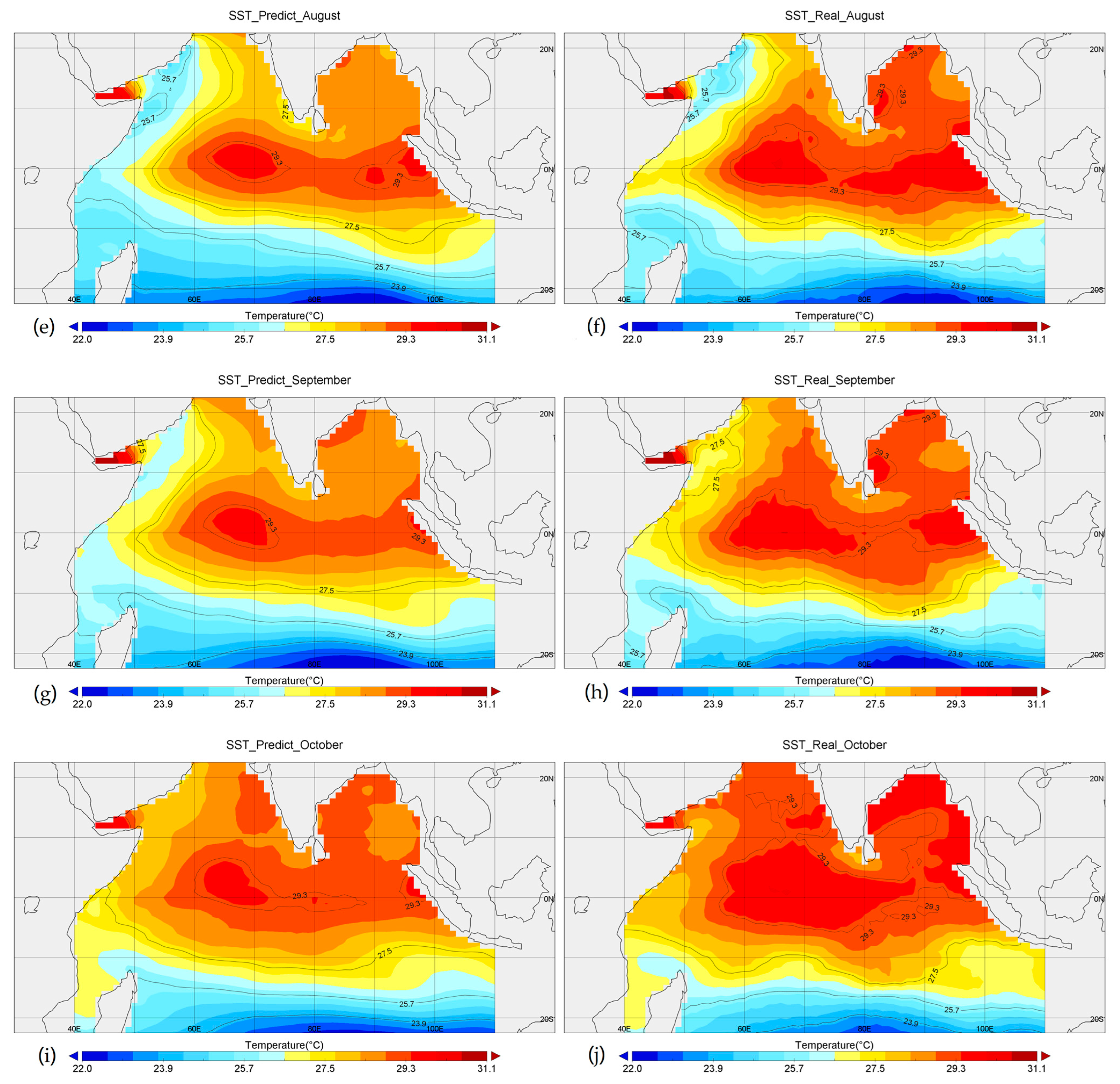
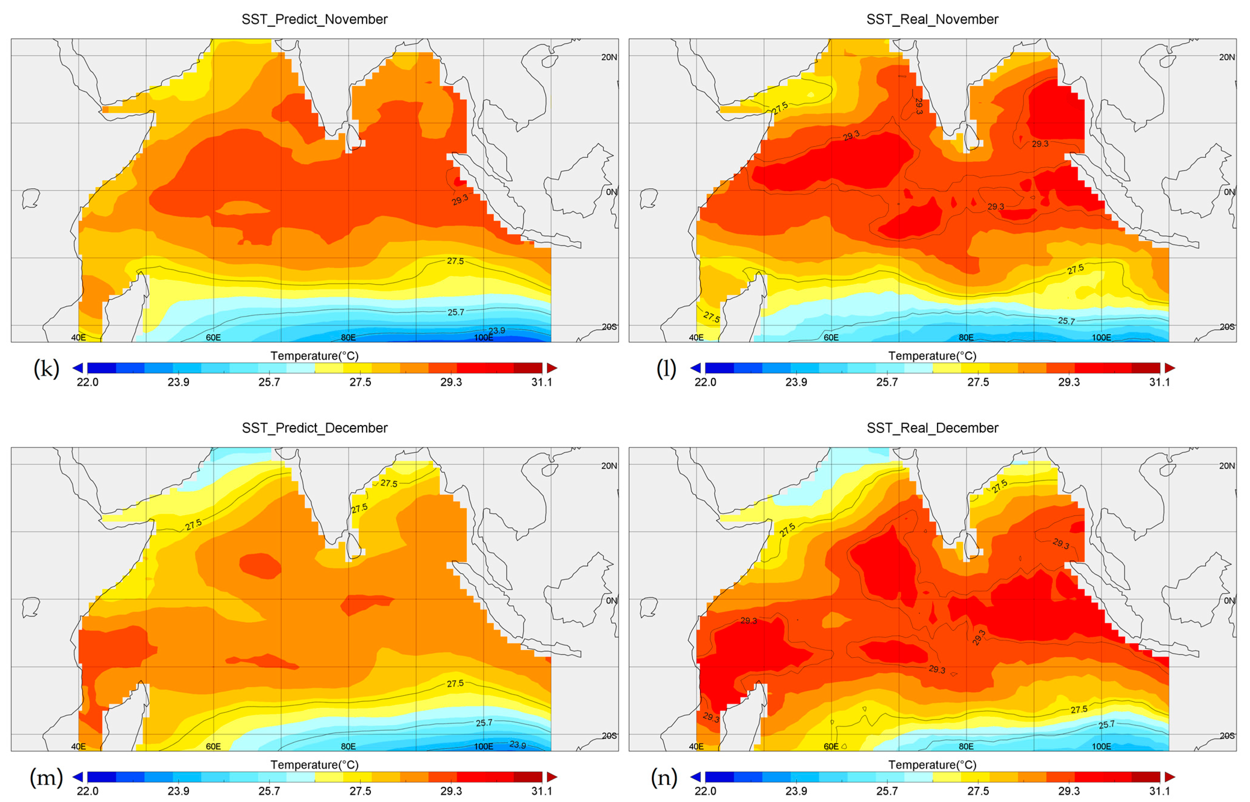
3. Results
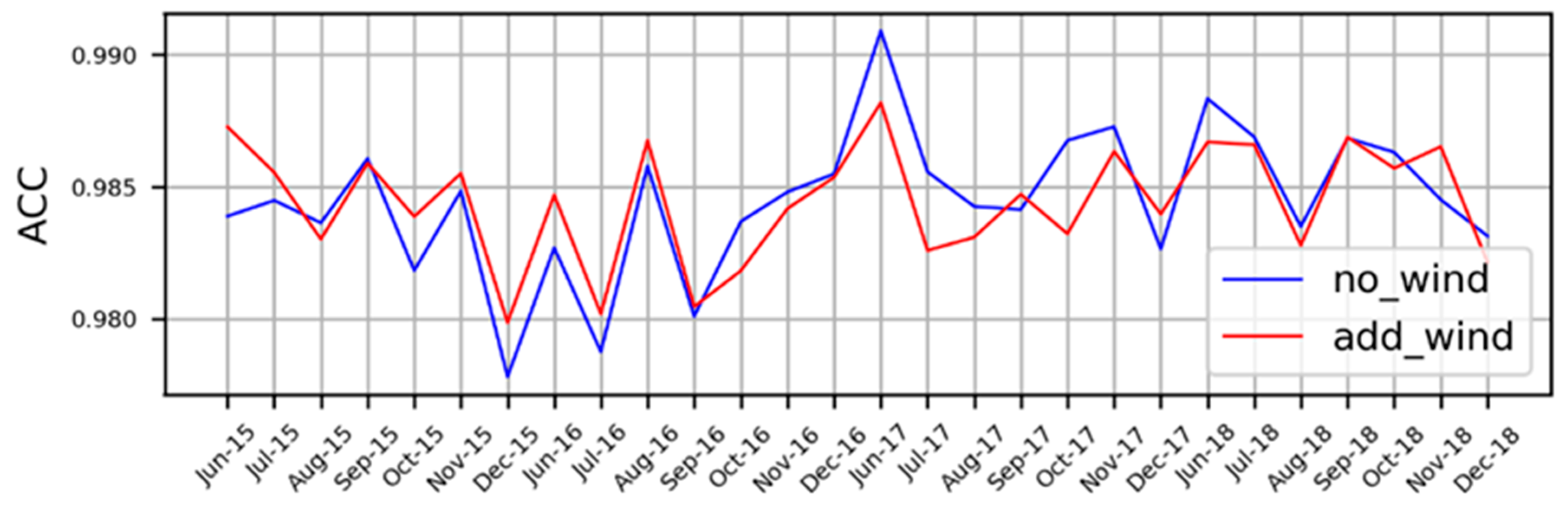
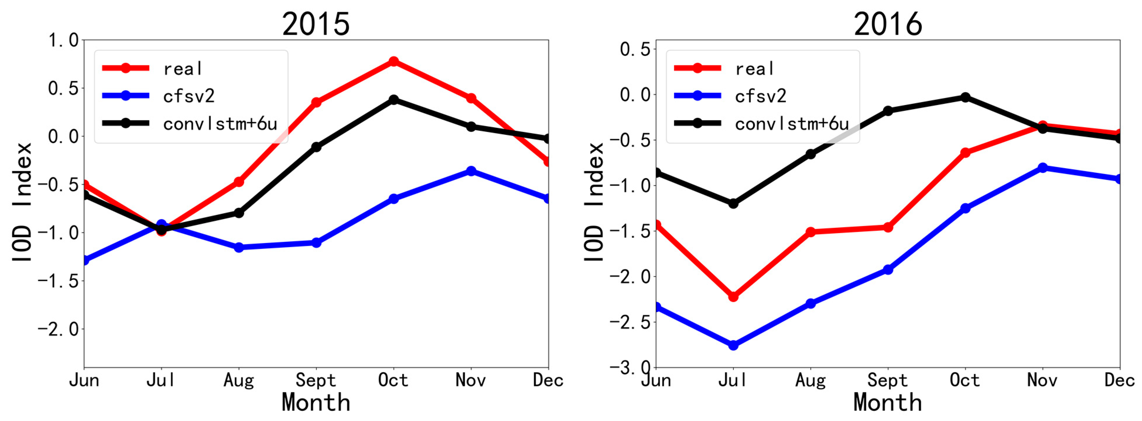
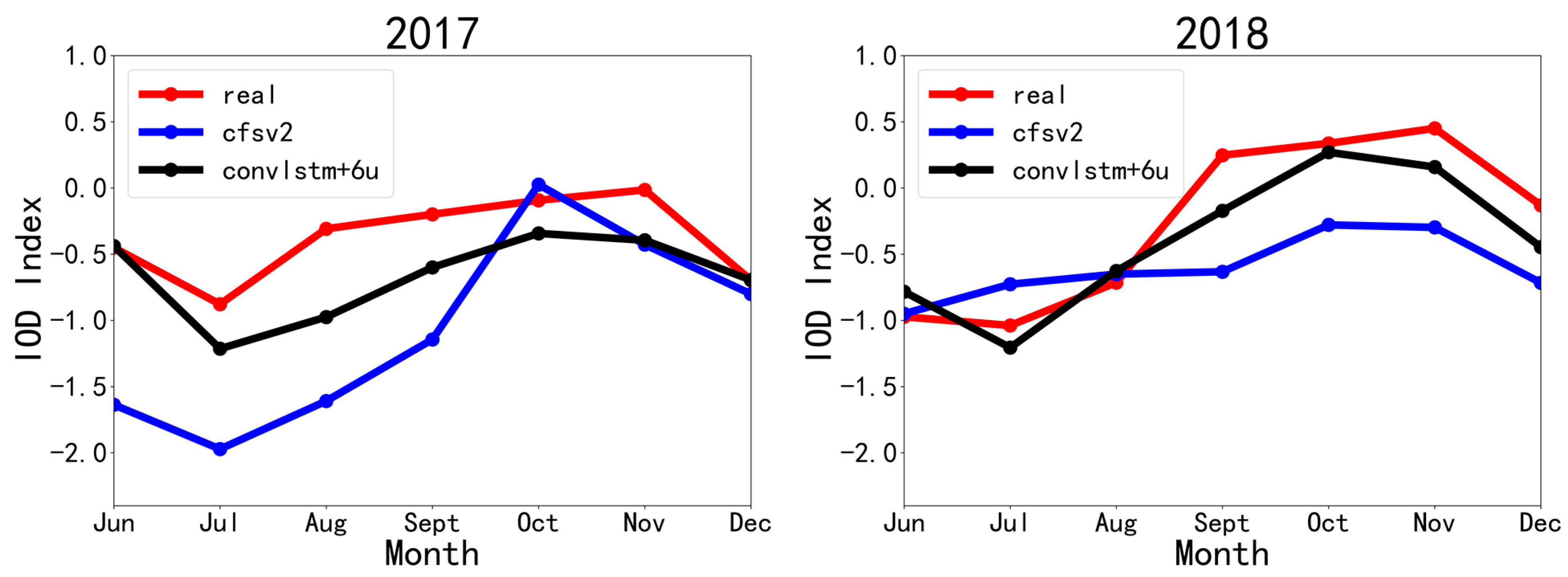
3.1. Comparison of RMSE and ACC
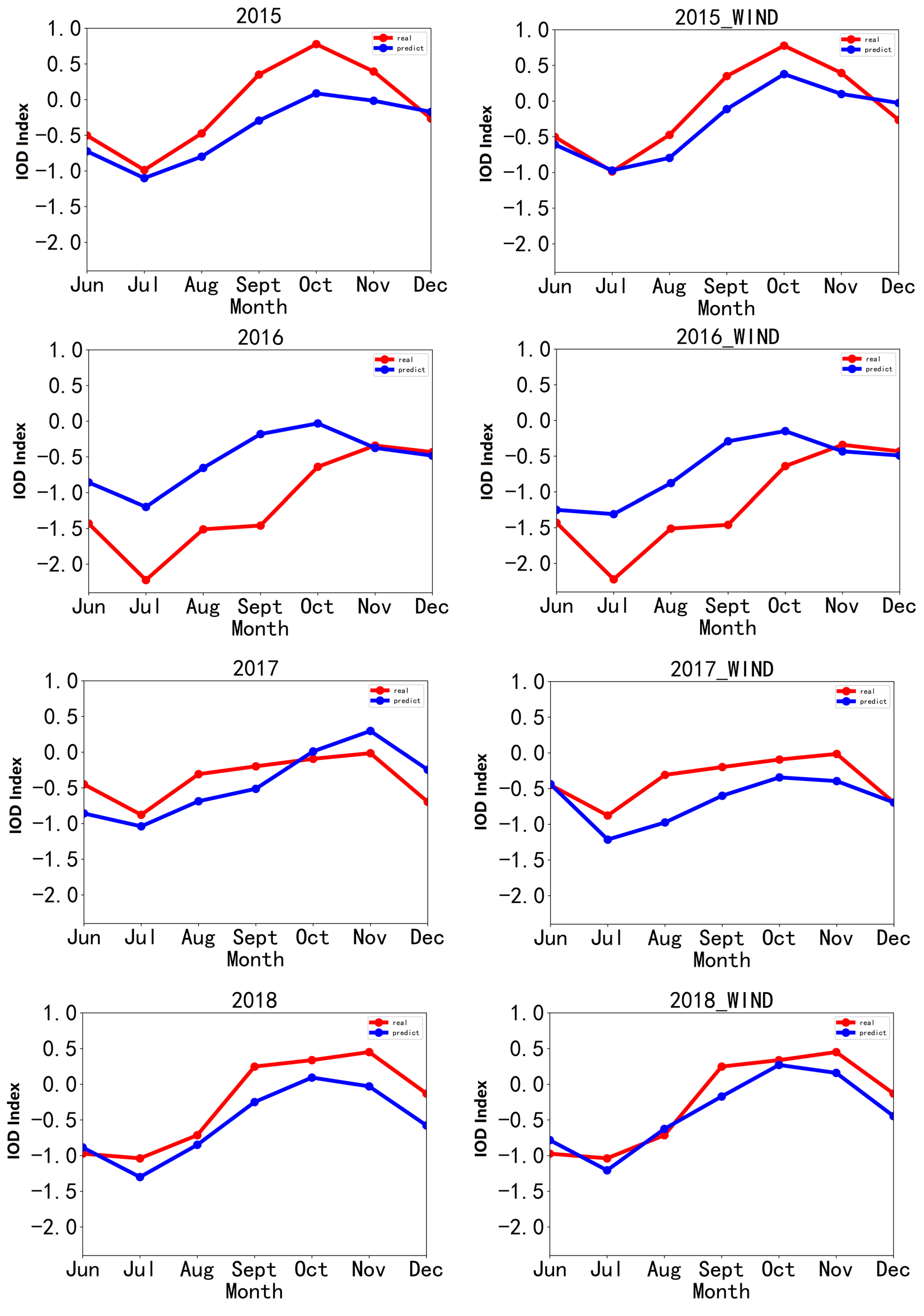
3.2. Correlation Coefficient between Real IOD Index and Predicted IOD Index
4. Discussion
5. Conclusions
Author Contributions
Funding
Data Availability Statement
Conflicts of Interest
References
- Saji, N.H.; Goswami, B.N.; Vinayachandran, P.N.; Yamagata, T. A dipole mode in the tropical Indian Ocean. Nature 1999, 401, 360–363. [Google Scholar] [CrossRef]
- Xiao, Y.; Zhang, Z.; He, J. Review on research progress of Indian Ocean Dipole. J. Trop. Meteorol. 2009, 25, 621–627. [Google Scholar]
- Wang, H.; Kumar, A.; Murtugudde, R.; Narapusetty, B.; Seip, K.L. Covariations between the Indian Ocean dipole and ENSO: A modeling study. Clim. Dyn. 2019, 53, 5743–5761. [Google Scholar] [CrossRef]
- Saji, N.H.; Yamagata, T. Possible impacts of Indian Ocean Dipole mode events on global climate. Clim. Res. 2003, 25, 151–169. [Google Scholar] [CrossRef]
- Ashok, K.; Guan, Z.; Saji, N.H.; Yamagata, T. Individual and combined infulences of ENSO and the Indian Ocean Dipole on the Indian summer monsoon. J. Clim. 2004, 17, 3141–3155. [Google Scholar] [CrossRef]
- Ashok, K.; Guan, Z.; Yamagata, T. Impact of the Indian Ocean Dipole on the relationship between the Indian monsoon rainfall and ENSO. Geophys. Res. Lett. 2001, 28, 4499–4502. [Google Scholar] [CrossRef] [Green Version]
- Behera, S.K.; Luo, J.; Masson, S.; Delecluse, P.; Gualdi, S.; Navarra, A.; Yamagata, T. Impact of the Indian Ocean Dipole on the East African short rains: A CGCM study. Clivar Exch. 2003, 27, 43–45. [Google Scholar] [CrossRef] [Green Version]
- Chan, S.C.; Behera, S.K.; Yamagata, T. Indian Ocean Dipole influence on South American rainfall. Geophys. Res. Lett. 2008, 35, L14S12. [Google Scholar] [CrossRef]
- Guan, Z.; Yamagata, T. The unusual summer of 1994 in East Asia: IOD teleconnections. Geophys. Res. Lett. 2003, 30, 235–250. [Google Scholar] [CrossRef] [Green Version]
- Qiu, Y.; Cai, W.; Guo, X.; Ng, B. The asymmetric influence of the positive and negative IOD events on China’s rainfall. Sci. Rep. 2014, 4, 4943. [Google Scholar] [CrossRef] [Green Version]
- Xiao, M.; Zhang, Q.; Singh, V.P. Influences of ENSO, NAO, IOD and PDO on seasonal precipitation regimes in the Yangtze River basin, China. Int. J. Climatol. 2015, 35, 3556–3567. [Google Scholar] [CrossRef]
- Xu, K.; Zhu, C.; Wang, W. The cooperative impacts of the El Niño–Southern Oscillation and the Indian Ocean Dipole on the interannual variability of autumn rainfall in China. Int. J. Climatol. 2016, 36, 1987–1999. [Google Scholar] [CrossRef] [Green Version]
- Wajsowicz, R.C. Climate variability over the tropical Indian Ocean sector in the NSIPP seasonal forecast system. J. Clim. 2004, 17, 4783–4804. [Google Scholar] [CrossRef]
- Wajsowicz, R.C. Seasonal-to-interannual forecasting of tropical Indian Ocean sea surface temperature anomalies: Potential predictability and barriers. J. Clim. 2007, 20, 3320–3343. [Google Scholar] [CrossRef]
- Luo, J.; Masson, S.; Behera, S.; Yamagata, T. Experimental forecasts of the Indian Ocean Dipole using a coupled OAGCM. J. Clim. 2007, 20, 2178–2190. [Google Scholar] [CrossRef]
- Zhao, M.; Hendon, H. Representation and prediction of the Indian Ocean Dipole in the POAMA seasonal forecast model. Q. J. R. Meteorol. Soc. 2009, 135, 337–352. [Google Scholar] [CrossRef]
- Bao, Q.; Wu, X.; Li, J.; Wang, L.; He, B.; Wang, X.; Liu, Y.; Wu, G. Prediction of El Nino and Indian Ocean Dipole in autumn and winter 2018–2019. Sci. Bull. 2019, 64, 73–78. [Google Scholar]
- Hu, S.; Wu, B.; Zhou, T. The reward technique of the recent climate prediction system iap-decpres for the Indian Ocean Dipole: A comparison between full field assimilation and anomaly field assimilation. Atmos. Sci. 2019, 43, 831–845. [Google Scholar]
- Zhao, S.; Jin, F.-F.; Stuecker, M.F. Improved Predictability of the Indian Ocean Dipole Using Seasonally Modulated ENSO Forcing Forecasts. Geophys. Res. Lett. 2019, 46, 9980–9990. [Google Scholar] [CrossRef]
- Ham, Y.G.; Kim, J.H.; Luo, J.J. Deep learning for multi-year ENSO forecasts. Nature 2019, 573, 568–572. [Google Scholar] [CrossRef]
- Sarkar, P.P.; Janardhan, P.; Roy, P. A novel deep neural network model approach to predict Indian Ocean dipole and Equatorial Indian Ocean oscillation indices. Dyn. Atmos. Oceans 2021, 96, 101266. [Google Scholar] [CrossRef]
- Lawrence, S.; Giles, C.L.; Tsoi, A.C.; Back, A.D. Face recognition: A convolutional neural-network approach. IEEE Trans. Neural Netw. 1997, 8, 98–113. [Google Scholar] [CrossRef] [PubMed] [Green Version]
- Swapna, A. Machine learning based sample extraction for automatic speech recognition using dialectal Assamese speech. Neural Netw. 2016, 78, 97–111. [Google Scholar]
- Xiong, J.; Bi, R.; Tian, Y.; Liu, X.; Wu, D. Towards Lightweight, Privacy-Preserving Cooperative Object Classification for Connected Autonomous Vehicles. IEEE Internet Things J. 2021, 1. [Google Scholar] [CrossRef]
- Xiong, J.; Bi, R.; Zhao, M.; Guo, J.; Yang, Q. Edge-Assisted Privacy-Preserving Raw Data Sharing Framework for Connected Autonomous Vehicles. IEEE Wirel. Commun. 2020, 27, 24–30. [Google Scholar] [CrossRef]
- Bi, R.; Chen, Q.; Xiong, J.; Liu, X. Design method of secure computing protocol for deep neural network. Chin. J. Netw. Inf. Secur. 2020, 6, 130–139. [Google Scholar]
- Zhang, Q.; Wang, H.; Dong, J.; Zhong, G.; Sun, X. Prediction of Sea Surface Temperature Using Long Short-Term Memory. IEEE Geosci. Remote Sens. Lett. 2017, 14, 1745–1749. [Google Scholar] [CrossRef] [Green Version]
- Krizhevsky, A.; Sutskever, I.; Hinton, G.E. ImageNet classification with deep convolutional neural networks. Commun. ACM 2017, 60, 84–90. [Google Scholar] [CrossRef]
- Shi, X.; Chen, Z.; Wang, H.; Yeung, D.-Y.; Wong, W.-K.; Woo, W. Convolutional LSTM Network: A Machine Learning Approach for Precipitation Nowcasting. arXiv 2015, arXiv:1506.04214. [Google Scholar]


| Parameters of atmosphere | |||||
| AT 1000hpa | AT 850hpa | AT 500hpa | AT 300hpa | GPH 1000hpa | GPH 850hpa |
| GPH 500hpa | GPH 300hpa | VV 1000hpa | VV 850hpa | VV 500hpa | VV 300hpa |
| RH1000hpa | RH 850hpa | RH 500hpa | RH 300hpa | ZWS 1000hpa | ZWS 850hpa |
| ZWS 500hpa | ZWS 300hpa | MWS 1000hpa | MWS 850hpa | MWS 500hpa | MWS 300hpa |
| Parameters of subsea | |||||
| SS 5m | SS 15m | SS 25m | SS 35m | SS 45m | SS 55m |
| SS 65m | SS 75m | SS 85m | SS 95m | u 5m | u 15m |
| u 25m | u 35m | u 45m | u 55m | u 65m | u 75m |
| u 85m | u 95m | v 5m | v 15m | v 25m | v 35m |
| v 45m | v 55m | v 65m | v 75m | v 85m | v 95m |
| ST 5m | ST 15m | ST 25m | ST 35m | ST 45m | ST 55m |
| ST 65m | ST 75m | ST 85m | ST 95m | ||
| Parameters of sea surface | |||||
| SST | sub1_SST | sub2_SST | sub3_SST | sub4_SST | sub5_SST |
| sub6_SST | sub7_SST | sub8_SST | sub9_SST | sub10_SST | sub11_SST |
| sub12_SST | sub13_SST | sub14_SST | sub15_SST | SSH | |
| Parameters of wind field | |||||
| sub1_U | sub2_U | sub3_U | sub4_U | sub5_U | sub6_U |
| sub7_U | sub8_U | sub9_U | sub10_U | sub11_U | sub12_U |
| sub13_U | sub14_U | sub15_U | |||
| RMSE Compare | 2015 | 2016 | 2017 | 2018 | ||||
|---|---|---|---|---|---|---|---|---|
| No_Wind | Wind | No_Wind | Wind | No_Wind | Wind | No_Wind | Wind | |
| Jun | 0.564 | 0.448 | 0.541 | 0.513 | 0.322 | 0.398 | 0.414 | 0.456 |
| Jul | 0.501 | 0.481 | 0.646 | 0.639 | 0.467 | 0.566 | 0.444 | 0.456 |
| Aug | 0.513 | 0.531 | 0.497 | 0.476 | 0.487 | 0.528 | 0.534 | 0.560 |
| Sept | 0.471 | 0.464 | 0.642 | 0.625 | 0.498 | 0.488 | 0.431 | 0.435 |
| Oct | 0.590 | 0.528 | 0.583 | 0.578 | 0.431 | 0.546 | 0.447 | 0.472 |
| Nov | 0.508 | 0.496 | 0.505 | 0.527 | 0.435 | 0.485 | 0.519 | 0.446 |
| Dec | 0.698 | 0.639 | 0.507 | 0.515 | 0.595 | 0.575 | 0.597 | 0.606 |
| Years | 2015 | 2016 | 2017 | 2018 | avg |
|---|---|---|---|---|---|
| convLSTM | 91.51% | 69.50% | 69.17% | 95.73% | 81.48% |
| convLSTM+6u | 92.24% | 72.24% | 72.36% | 94.52% | 82.84% |
| CFSv2 | 49.33% | 97.67% | 65.53% | 80.53% | 73.27% |
Publisher’s Note: MDPI stays neutral with regard to jurisdictional claims in published maps and institutional affiliations. |
© 2022 by the authors. Licensee MDPI, Basel, Switzerland. This article is an open access article distributed under the terms and conditions of the Creative Commons Attribution (CC BY) license (https://creativecommons.org/licenses/by/4.0/).
Share and Cite
Li, C.; Feng, Y.; Sun, T.; Zhang, X. Long Term Indian Ocean Dipole (IOD) Index Prediction Used Deep Learning by convLSTM. Remote Sens. 2022, 14, 523. https://doi.org/10.3390/rs14030523
Li C, Feng Y, Sun T, Zhang X. Long Term Indian Ocean Dipole (IOD) Index Prediction Used Deep Learning by convLSTM. Remote Sensing. 2022; 14(3):523. https://doi.org/10.3390/rs14030523
Chicago/Turabian StyleLi, Chen, Yuan Feng, Tianying Sun, and Xingzhi Zhang. 2022. "Long Term Indian Ocean Dipole (IOD) Index Prediction Used Deep Learning by convLSTM" Remote Sensing 14, no. 3: 523. https://doi.org/10.3390/rs14030523
APA StyleLi, C., Feng, Y., Sun, T., & Zhang, X. (2022). Long Term Indian Ocean Dipole (IOD) Index Prediction Used Deep Learning by convLSTM. Remote Sensing, 14(3), 523. https://doi.org/10.3390/rs14030523