
Siamese Detail Difference and Self-Inverse Network for Forest Cover Change Extraction Based on Landsat 8 OLI Satellite Images

 ,
,  , and
, and
Abstract
:1. Introduction
2. Related Work
3. Methodology
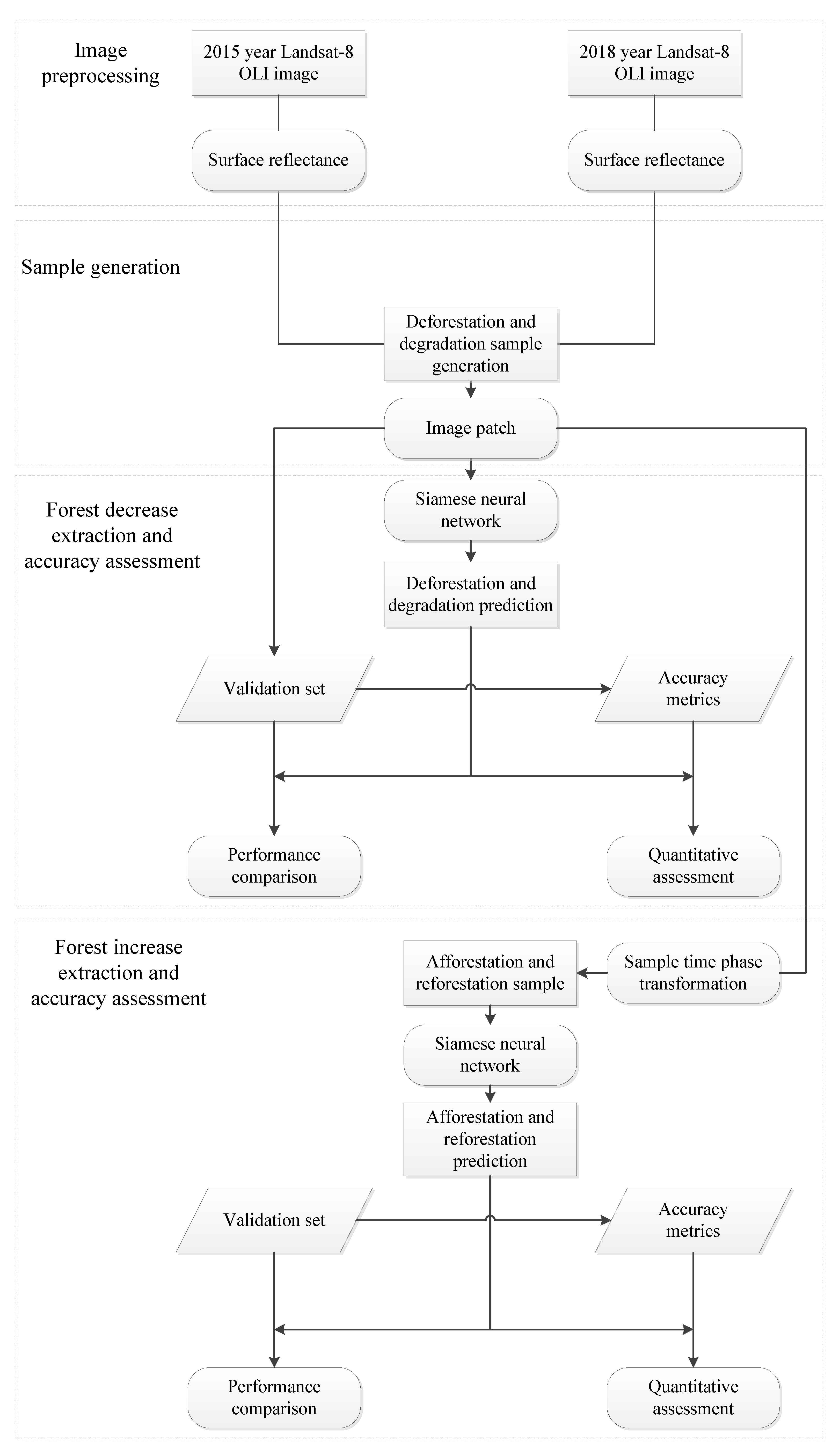
3.1. Overview
- (1)
- Suface reflectance calculation. In order to make the images of different time comparable, the digital number (DN) value of the images used in the experiment are converted into surface reflectance. The LEDAPS and LaSRC surface reflectance algorithms released by NASA/GSFC and the University of Maryland [78,79] is used to calculate the surface reflectance in this study.
- (2)
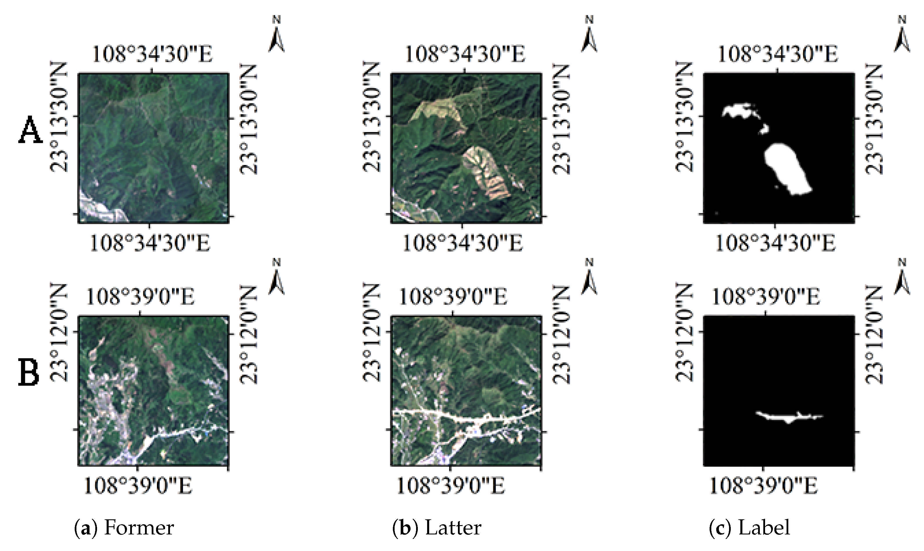
- Sample generation. The deforestation and degradation samples are generated and clipped into image patches. In this process, the surface reflectance images are aligned according to coordinates and manually labeled to create sample images. Thus, the remote sensing images and sample images are clipped into patches.
- (3)
- Forest decrease extraction. Two new versions of the Siamese neural networks are proposed to predict forest decrease. They are Fully Convolutional Siamese Global Difference network (FCGD) and Fully Convolutional Siamese Detail Difference network (FCDD). See Section 3.2 for details. The surface reflectance variables of the six bands (blue, green, red, near-infrared and two mid-infrared bands) in the labeled pixel are input into these models. The accuracy comparison of different methods are conducted using quantitative evaluation metrics. The extraction results in the various deforestation and degradation region are analyzed visually.
- (4)
- Forest increase extraction. Self-inverse networks are designed for forest increase extraction. See Section 3.3 for details. The forest decrease sample dataset is reversed in time phase and imported into the network used in the forest decrease prediction. Without changing the architecture of the networks, the Siamese neural networks are trained by the same sample and tested for forest increase extraction.
3.2. The Structure of the Proposed Siamese Neural Network
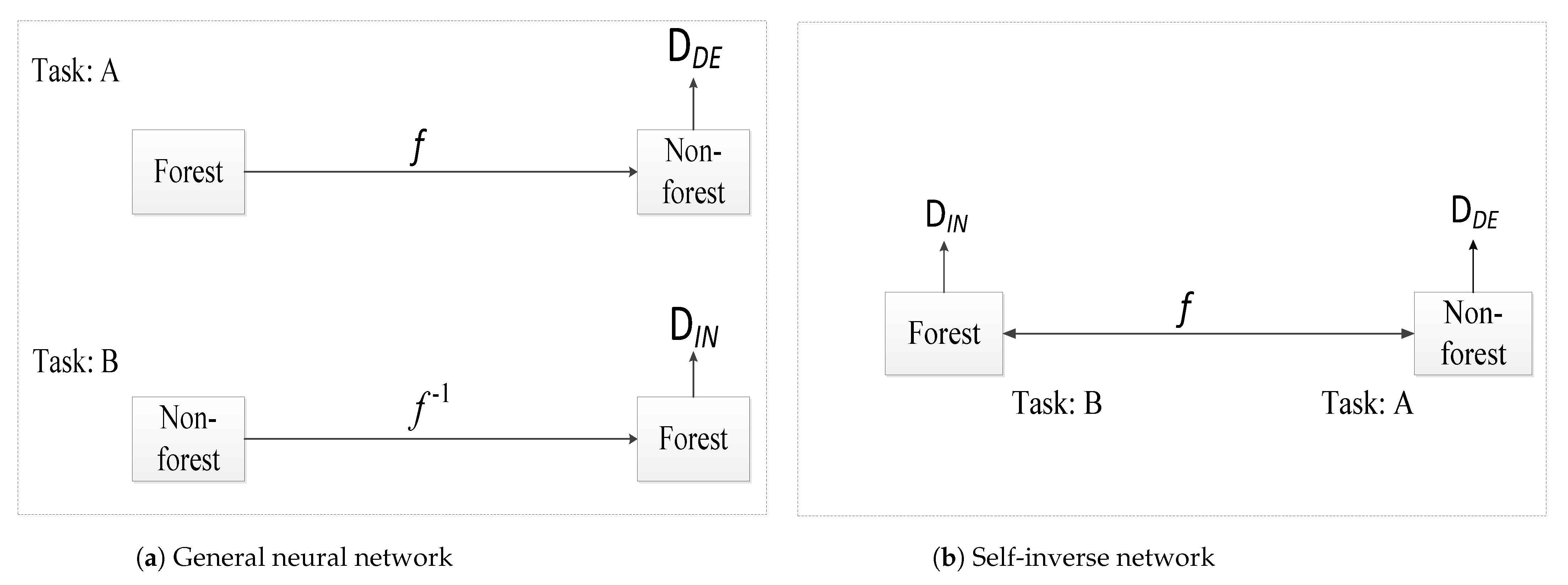
3.3. Self-Inverse Network
3.4. Data Augmentation
4. Experiments and Results Analysis
4.1. Implementation Details
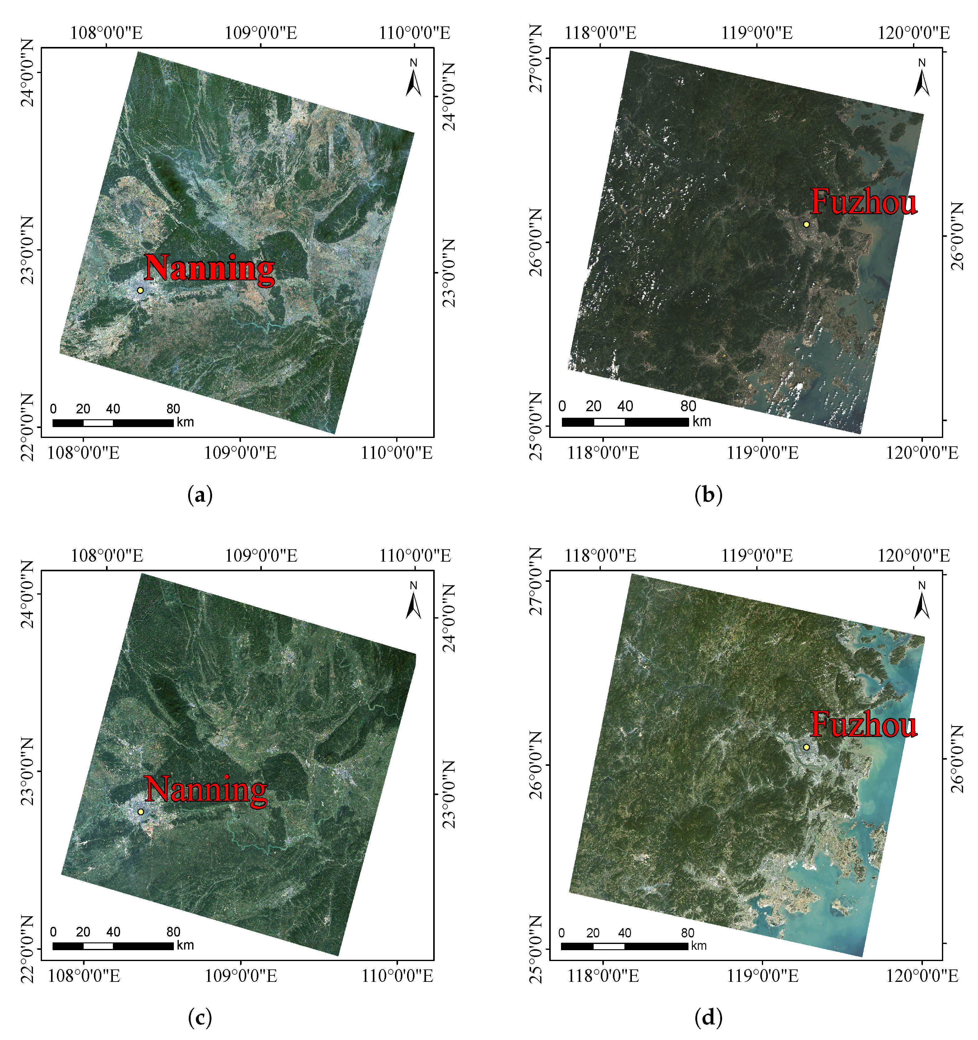
4.1.1. Datasets
4.1.2. The Creation of Training Dataset
4.1.3. Evaluation Metrics
4.2. Comparison of Forest Decrease
4.2.1. Quantitative Analysis
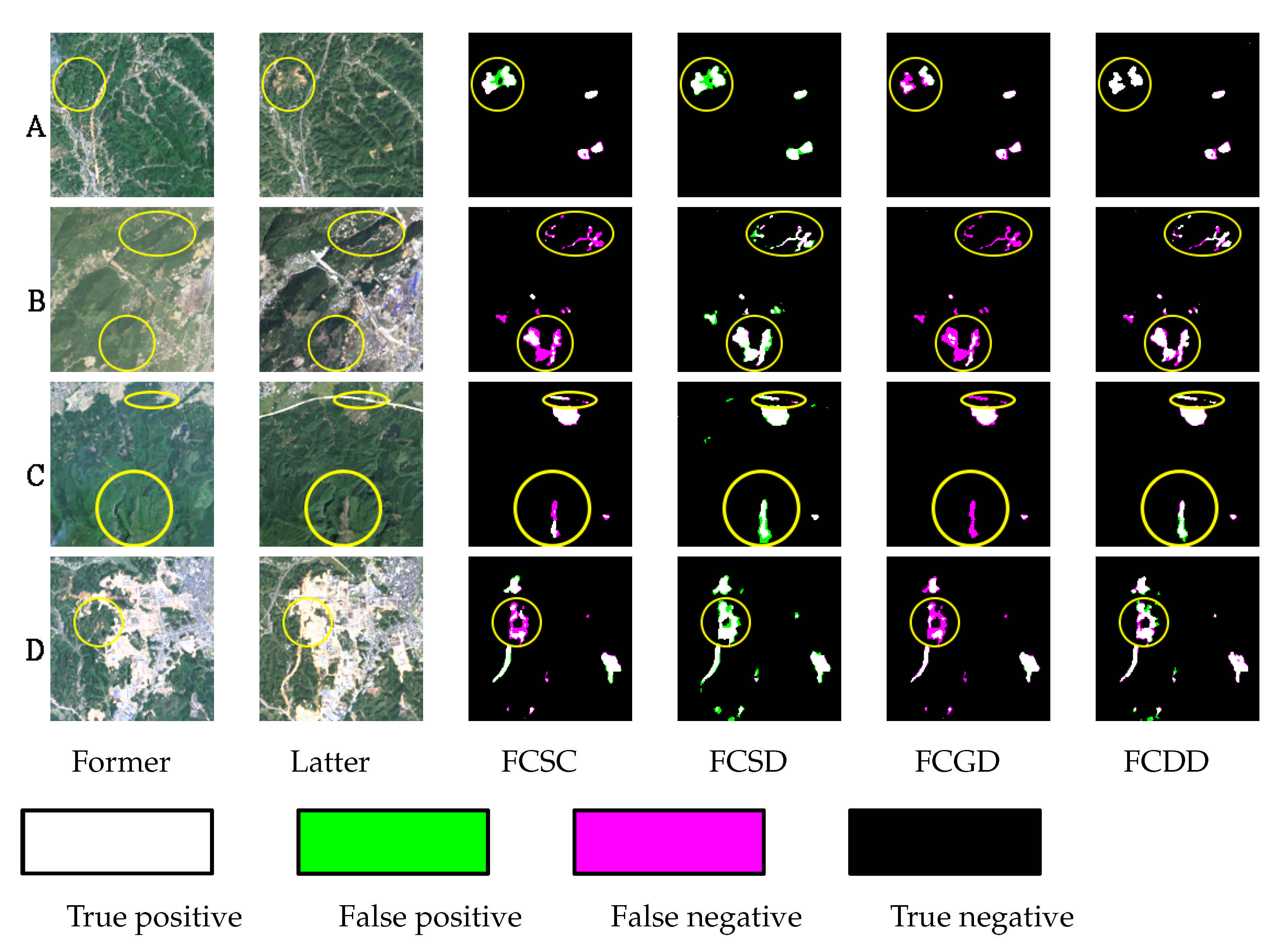
4.2.2. Qualitative Analysis
4.3. Comparison of Forest Increase
4.3.1. Quantitative Analysis
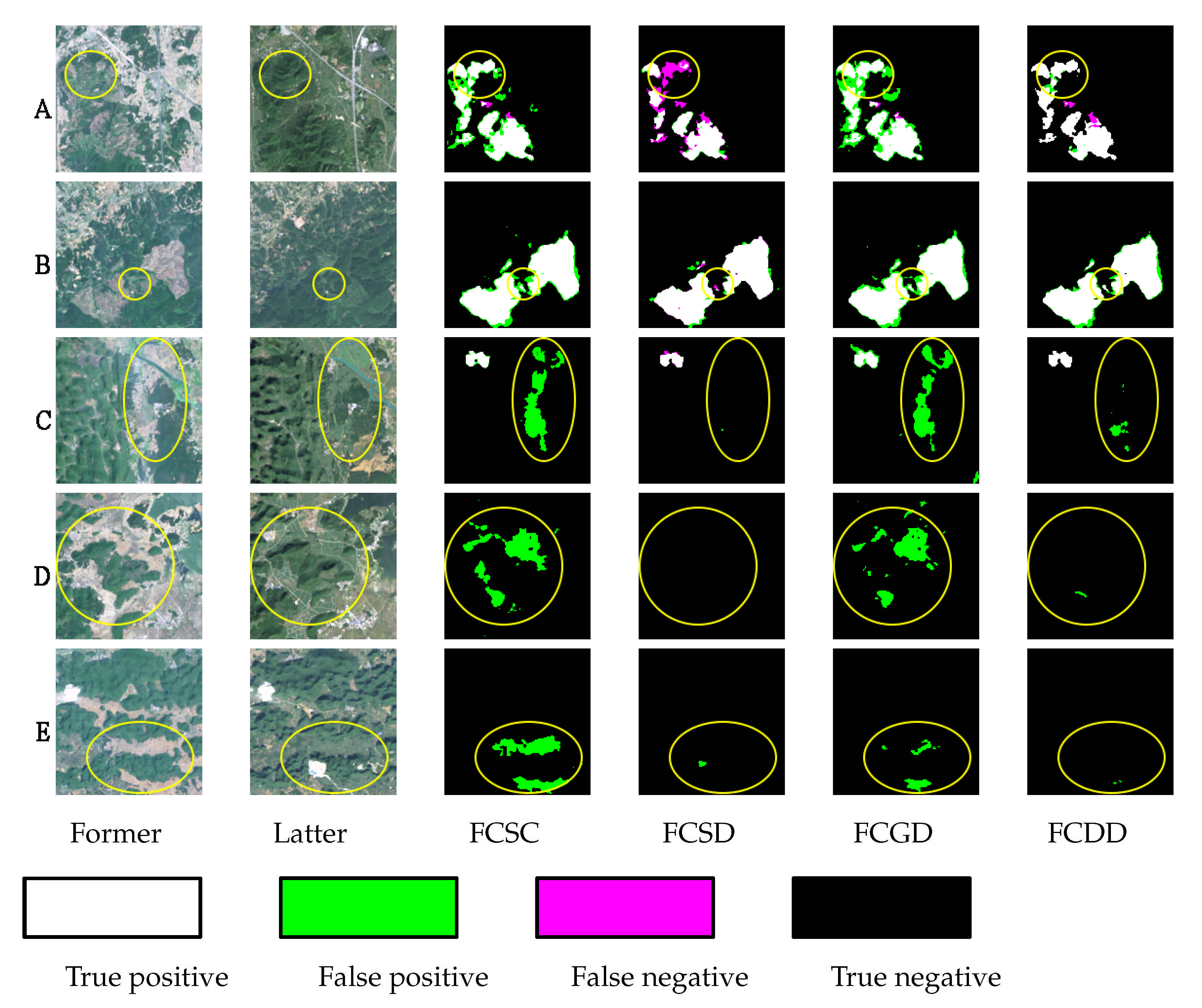
4.3.2. Qualitative Analysis
5. Discussion
- (1)
- Improvement compared with traditional Siamese neural networks. In this study, the classification accuracy of forest decrease and increase in two regions is evaluated through qualitative and quantitative analysis. The results demonstrate that the classification accuracy of subtract weight mode FCDD in various forest cover change is higher than that of concatenate and subtract weight sharing mode in FCSC and FCSD. Subsequently, the performance of subtract weight sharing mode in eliminating noise of forest increase is better than that of concatenate weight sharing mode. This phenomenon is due to the fact that the subtract weight sharing mode is more able to use the different information for forest change extraction than the concatenate weight sharing mode. Due to the fully concatenation weight sharing mode, FCSC extracts two phase information and lacks focus of change information. Due to the fully subtraction weight sharing mode, FCSD is designed to focus on the change information between two phase and extracts some pseudo-change information in the same time. Combining the above weight sharing mode, FCDD has the ability of utilizing different information and pseudo-change information simultaneously.
- (2)
- Differences between FCDD and FCGD. As two types of Siamese neural network, FCDD and FCGD have obvious differences in the theoretical method and experiment results. In the theoretical method, FCDD has a concatenation weight sharing mode in the top layer of downsampling process, while the other layers are made by subtract weight sharing mode. In the downsampling process of FCGD, the top layer is a subtract weight sharing mode, and the other layers are a concatenate weight sharing mode. In the experiment results, FCDD has better capability of noise eliminating than FCGD, such as shrub wither and grass wilt. The subtract weight sharing mode in the more subtle convolutional layers gives FCDD better forest cover change detection ability. As the break-even point of precision and recall, F-measure shows the quantitative performance measure of predict results. FCDD has the best F-measure score in forest decrease and increase extraction experiments, following by FCSC and FCGD. This difference approves that given the same forest change image, FCDD has better ability in predicting forest cover change than FCGD.
- (3)
- Self-inverse network. In the field of remote sensing, it is the first time that self-inverse network is used for forest cover change detection. In such a bidirectional change field, the self-inverse network experiment not only reduces the generation cost of training data, but also extends universality of classification architecture model. According to the results in the paper, the Siamese neural network has proven its accurate detection capacity and compatible universality in forest cover translation. The types of features before and after forest decrease and increase are not completely equal, thus forest decrease and increase are not completely reversible. The feature types after the forest decrease include the feature types before the increase, which allows the sample of the forest decrease to be used for training increase. However, lacking the combination of the bi-temporal feature information and the difference information, the traditional Siamese neural networks (FCSC and FCSD) perform poorly in self-inverse prediction. On the other hand, the novel fused weight sharing strategies make the proposed Siamese neural networks FCDD more robust to be applied to a self-inverse task.
- (4)
- Factors affecting accuracy. In the whole process of forest cover change detection, there are several factors affecting accuracy. The first factor is image preprocessing. To ensure data consistency, most change detection maps are based on the top of atmosphere (TOA) reflectance or surface reflectance. However, due to various shooting time and geographic variation, the surface reflectance of image collection exists difference, which influences control variables of the change information extraction. Secondly, the forest decrease training dataset includes some kinds of deforestation that doesn’t exist in the reforestation. This situation leads to the problem that the training dataset of deforestation and reforestation is incompletely self-inverse. The reforestation samples are improper for self-inverse deforestation experiment. Otherwise, various mixtures between the forest change and unchange areas exist.
- (5)
- Training samples generation. In order to select accurate samples of forest cover changes in the complex surface, this experiment combined Landsat medium-resolution images and Google Earth high-resolution images to manually label the forest decrease and increase samples. However, this process limits the automatic processing capacity of the proposed algorithm. This problem shows that various types of typical forest cover change samples will be the main demand for future work.
- (1)
- A novel weight sharing mode of a Siamese neural network based on U-Net for forest cover change detection is proposed, and this method obtains promising classification results.
- (2)
- Self-inverse network of Siamese architecture is generated. According to the self-inverse network, forest decrease sample dataset is used for change detection in forest increase, which implements transfer learning of sample dataset and improves the utilization rate of sample dataset.
6. Conclusions
- (1)
- Based on a visual comparison, the performance of the Siamese detail difference neural network extracting forest cover change is better than those of Siamese concatenate neural network, Siamese difference neural network and Siamese global difference neural network. Moreover, quantitative evaluation shows that the overall accuracy and kappa coefficients of FCDD are higher than those of the other three classifiers. The kappa coefficients of FCDD in forest decrease and increase extraction experiments are 82.55% and 81.69%, and the F-measures and IoUs of those are 0.8280 and 0.8181, 0.7064 and 0.6923.
- (2)
- Compared with FCSC, FCSD and FCGD, the performance of FCDD demonstrates that it can precisely extract three types of large forest decrease areas (i.e., large roads and infrastructure projects, urban expand and logging), and detailed deforestation can also be identified. Furthermore, FCDD can effectively eliminate noise, such as grassland and shrub perishment.
- (3)
- In the forest increase extraction, FCDD has the advantage of self-inverse function learning the principle of forest transfer to non-forest. Trained by the existed forest decrease dataset, FCDD has the capacity of detecting forest increase without the effort of amending neural network parameters.
Author Contributions
Funding
Institutional Review Board Statement
Informed Consent Statement
Data Availability Statement
Conflicts of Interest
References
- Hansen, M.C.; Potapov, P.V.; Moore, R.; Hancher, M.; Turubanova, S.A.; Tyukavina, A.; Townshend, J. High-resolution global maps of 21st-century forest cover change. Science 2013, 342, 850–853. [Google Scholar] [CrossRef] [PubMed] [Green Version]
- Feng, M.; Sexton, J.O.; Huang, C.; Anand, A.; Channan, S.; Song, X.P.; Townshend, J.R. Earth science data records of global forest cover and change: Assessment of accuracy in 1990, 2000, and 2005 epochs. Remote Sens. Environ. 2016, 184, 73–85. [Google Scholar] [CrossRef] [Green Version]
- Curtis, P.G.; Slay, C.M.; Harris, N.L.; Tyukavina, A.; Hansen, M.C. Classifying drivers of global forest loss. Science 2018, 361, 1108–1111. [Google Scholar] [CrossRef]
- Houghton, R.A. Historic role of forests in the global carbon cycle. In Carbon Dioxide Mitigation in Forestry and Wood Industry; Springer: Berlin/Heidelberg, Germany, 1998; pp. 1–24. [Google Scholar]
- Song, X.P.; Huang, C.; Saatchi, S.S.; Hansen, M.C.; Townshend, J.R. Annual carbon emissions from deforestation in the Amazon Basin between 2000 and 2010. PLoS ONE 2015, 10, e0126754. [Google Scholar] [CrossRef] [PubMed] [Green Version]
- Woodward, C.; Shulmeister, J.; Larsen, J.; Jacobsen, G.E.; Zawadzki, A. The hydrological legacy of deforestation on global wetlands. Science 2014, 346, 844–847. [Google Scholar] [CrossRef] [PubMed] [Green Version]
- Haddad, N.M.; Brudvig, L.A.; Clobert, J.; Davies, K.F.; Gonzalez, A.; Holt, R.D.; Townshend, J.R. Habitat fragmentation and its lasting impact on Earth’s ecosystems. Sci. Adv. 2015, 1, e1500052. [Google Scholar] [CrossRef] [PubMed] [Green Version]
- Smart, L.S.; Swenson, J.J.; Christensen, N.L.; Sexton, J.O. Three-dimensional characterization of pine forest type and red-cockaded woodpecker habitat by small-footprint, discrete-return lidar. For. Ecol. Manag. 2012, 281, 100–110. [Google Scholar] [CrossRef]
- Zuluaga, G.J.C.; Rodewald, A.D. Response of mixed-species flocks to habitat alteration and deforestation in the Andes. Biol. Conserv. 2015, 188, 72–81. [Google Scholar] [CrossRef]
- Barber, C.P.; Cochrane, M.A.; Souza Jr, C.M.; Laurance, W.F. Roads, deforestation, and the mitigating effect of protected areas in the Amazon. Biol. Conserv. 2014, 177, 203–209. [Google Scholar] [CrossRef]
- Laumonier, Y.; Uryu, Y.; Stüwe, M.; Budiman, A.; Setiabudi, B.; Hadian, O. Eco-floristic sectors and deforestation threats in Sumatra: Identifying new conservation area network priorities for ecosystem-based land use planning. Biodivers. Conserv. 2010, 19, 1153–1174. [Google Scholar] [CrossRef]
- Etter, A.; McAlpine, C.; Wilson, K.; Phinn, S.; Possingham, H. Regional patterns of agricultural land use and deforestation in Colombia. Agric. Ecosyst. Environ. 2006, 114, 369–386. [Google Scholar] [CrossRef]
- Pahari, K.; Murai, S. Modelling for prediction of global deforestation based on the growth of human population. ISPRS J. Photogramm. Remote Sens. 1999, 54, 317–324. [Google Scholar] [CrossRef]
- Hansen, M.C.; DeFries, R.S. Detecting long-term global forest change using continuous fields of tree-cover maps from 8-km advanced very high resolution radiometer (AVHRR) data for the years 1982–1999. Ecosystems 2004, 7, 695–716. [Google Scholar] [CrossRef]
- Renó, V.F.; Novo, E.M.; Suemitsu, C.; Rennó, C.D.; Silva, T.S. Assessment of deforestation in the Lower Amazon floodplain using historical Landsat MSS/TM imagery. Remote Sens. Environ. 2011, 115, 3446–3456. [Google Scholar] [CrossRef]
- Thiel, C.; Thiel, C.; Riedel, T.; Schmullius, C. Object based classification of SAR data for the delineation of forest cover maps and the detection of deforestation—A viable procedure and its application in GSE Forest Monitoring. In Object-Based Image Analysis; Springer: Berlin/Heidelberg, Germany, 2008; pp. 327–343. [Google Scholar]
- Kim, D.H.; Sexton, J.O.; Noojipady, P.; Huang, C.Q.; An, A.; Channan, S.; Feng, M.; Townshend, J.R. Global, Landsat-based forest-cover change from 1990 to 2000. Remote Sens. Environ. 2014, 155, 178–193. [Google Scholar] [CrossRef] [Green Version]
- Huang, X.M.; Fied, M.A. Distance metric-based forest cover change detection using MODIS time series. Int. J. Appl. Earth Obs. Geoinf. 2014, 29, 78–92. [Google Scholar] [CrossRef]
- Qin, Y.W.; Xiao, X.M.; Wang, J.; Dong, J.W.; Ewing, K.T.; Hoagl, B.; Hough, D.J.; Fagin, T.D.; Zou, Z.H.; Geissler, G.L.; et al. Mapping Annual Forest Cover in Sub-Humid and Semi-Arid Regions through Analysis of Landsat and PALSAR Imagery. Remote Sens. 2016, 8, 933. [Google Scholar] [CrossRef] [Green Version]
- De Filho, F.J.B.O.; Metzger, J.P. Thresholds in landscape structure for three common deforestation patterns in the Brazilian Amazon. Landsc. Ecol. 2006, 21, 1061–1073. [Google Scholar] [CrossRef]
- Huete, A.; Didan, K.; Miura, T.; Rodriguez, E.P.; Gao, X.; Ferreira, L.G. Overview of the radiometric and biophysical performance of the MODIS vegetation indices. Remote Sens. Environ. 2002, 83, 195–213. [Google Scholar] [CrossRef]
- Huete, A.; Justice, C.; Liu, H. Development of vegetation and soil indices for MODIS-EOS. Remote Sens. Environ. 2002, 49, 224–234. [Google Scholar] [CrossRef]
- Huete, A.R.; Liu, H.Q.; Batchily, K.; Van Leeuwen, W. A comparison of vegetation indices over a global set of TM images for EOS-MODIS. Remote Sens. Environ. 1997, 59, 440–451. [Google Scholar] [CrossRef]
- Pinty, B.; Verstraete, M.M. GEMI: A non-linear index to monitor global vegetation from satellites. Vegetation 1992, 101, 15–20. [Google Scholar] [CrossRef]
- Souza, C.M., Jr.; Siqueira, J.V.; Sales, M.H.; Fonseca, A.V.; Ribeiro, J.G.; Numata, I.; Cochrane, M.A.; Barber, C.P.; Roberts, D.A.; Barlow, J. Ten-year landsat classification of deforestation and forest degradation in the brazilian amazon. Remote Sens. 2013, 5, 5493–5513. [Google Scholar] [CrossRef] [Green Version]
- Carlos, S.M., Jr.; Roberts, D.A.; Cochrane, M.A. Combining spectral and spatial information to map canopy damage from selective logging and forest fires. Remote Sens. Environ. 2005, 98, 329–343. [Google Scholar] [CrossRef]
- Jin, S.; Sader, S.A. Comparison of time series tasseled cap wetness and the normalized difference moisture index in detecting forest disturbances. Remote Sens. Environ. 2005, 94, 364–372. [Google Scholar] [CrossRef]
- Goodwin, N.R.; Coops, N.C.; Wulder, M.A.; Gillanders, S.; Schroeder, T.A.; Nelson, T. Estimation of insect infestation dynamics using a temporal sequence of Landsat data. Remote Sens. Environ. 2008, 112, 3680–3689. [Google Scholar] [CrossRef]
- Hayes, D.J.; Cohen, W.B.; Sader, S.A.; Irwin, D.E. Estimating proportional change in forest cover as a continuous variable from multi-year MODIS data. Remote Sens. Environ. 2008, 112, 735–749. [Google Scholar] [CrossRef] [Green Version]
- Tucker, C.J. Red and photographic infrared linear combinations for monitoring vegetation. Remote Sens. Environ. 1979, 8, 127–150. [Google Scholar] [CrossRef] [Green Version]
- DeVries, B.; Verbesselt, J.; Kooistra, L.; Herold, M. Robust monitoring of small-scale forest disturbances in a tropical montane forest using Landsat time series. Remote Sens. Environ. 2015, 161, 107–121. [Google Scholar] [CrossRef]
- Miura, T.; Huete, A.R.; Van Leeuwen, W.J.D.; Didan, K. Vegetation detection through smoke-filled AVIRIS images: An assessment using MODIS band passes. J. Geophys. Res. Atmos. 1998, 103, 32001–32011. [Google Scholar] [CrossRef]
- Schultz, M.; Clevers, J.G.; Carter, S.; Verbesselt, J.; Avitabile, V.; Quang, H.V.; Herold, M. Performance of vegetation indices from Landsat time series in deforestation monitoring. Int. J. Appl. Earth Obs. Geoinf. 2016, 52, 318–327. [Google Scholar] [CrossRef]
- Chen, G.; Hay, G.J.; Carvalho, L.M.; Wulder, M.A. Object-based change detection. Int. J. Remote Sens. 2012, 33, 4434–4457. [Google Scholar] [CrossRef]
- Heurich, M.; Ochs, T.; Resen, T.; Schneider, T. Object-orientated image analysis for the semi-automatic detection of dead trees following a spruce bark beetle (Ips typographus) outbreak. Eur. J. For. Res. 2010, 129, 313–324. [Google Scholar] [CrossRef]
- Hese, S.; Schmullius, C. Approaches to KYOTO Afforestation, Reforestation and Deforestation Mapping in Siberia using Object Oriented Change Detection Methods. In Hazard Ecology: Approaches and Techniques; Mittal Publications: Delhi, India, 2010; p. 77. [Google Scholar]
- Guild, L.S.; Cohen, W.B.; Kauffman, J.B. Detection of deforestation and land conversion in Rondônia, Brazil using change detection techniques. Int. J. Remote Sens. 2004, 25, 731–750. [Google Scholar] [CrossRef]
- Longépé, N.; Rakwatin, P.; Isoguchi, O.; Shimada, M.; Uryu, Y.; Yulianto, K. Assessment of ALOS PALSAR 50 m Orthorectified FBD Data for Regional Land Cover Classification by Support Vector Machines. IEEE Trans. Geosci. Remote Sens. 2011, 49, 2135–2150. [Google Scholar] [CrossRef]
- Huang, C.; Song, K.; Kim, S.; Townshend, J.R.; Davis, P.; Masek, J.G.; Goward, S.N. Use of a dark object concept and support vector machines to automate forest cover change analysis. Remote Sens. Environ. 2008, 112, 970–985. [Google Scholar] [CrossRef]
- DeFries, R.S.; Chan, J.C.W. Multiple Criteria for Evaluating Machine Learning Algorithms for Land Cover Classification from Satellite Data. Remote Sens. Environ. 2000, 74, 503–515. [Google Scholar] [CrossRef]
- Hosonuma, N.; Herold, M.; De Sy, V.; De Fries, R.S.; Brockhaus, M.; Verchot, L.; Romijn, E. An assessment of deforestation and forest degradation drivers in developing countries. Environ. Res. Lett. 2012, 7, 044009. [Google Scholar] [CrossRef]
- Jin, Y.; Sung, S.; Lee, D.K.; Biging, G.S.; Jeong, S. Mapping Deforestation in North Korea Using Phenology-Based Multi-Index and Random Forest. Remote Sens. 2016, 8, 997. [Google Scholar] [CrossRef] [Green Version]
- Bueno, I.T.; Acerbi Júnior, F.W.; Silveira, E.M.O.; Mello, J.M.; Carvalho, L.M.T.; Gomide, L.R.; Withey, K.; Scolforo, J.R.S. Object-Based Change Detection in the Cerrado Biome Using Landsat Time Series. Remote Sens. 2019, 11, 570. [Google Scholar] [CrossRef] [Green Version]
- Mas, J.F.; Puig, H.; Palacio, J.L.; Sosa-López, A. Modelling deforestation using GIS and artificial neural networks. Environ. Model. Softw. 2004, 19, 461–471. [Google Scholar] [CrossRef]
- Nunes Kehl, T.; Todt, V.; Veronez, M.R.; Cazella, S.C. Amazon Rainforest Deforestation Daily Detection Tool Using Artificial Neural Networks and Satellite Images. Sustainability 2012, 4, 2566–2573. [Google Scholar] [CrossRef] [Green Version]
- Maretto, R.V.; Fonseca, L.M.; Jacobs, N.; Körting, T.S.; Bendini, H.N.; Parente, L.L. Spatio-Temporal Deep Learning Approach to Map Deforestation in Amazon Rainforest. IEEE Geosci. Remote Sens. Lett. 2020, 18, 771–775. [Google Scholar] [CrossRef]
- Mayfield, H.J.; Smith, C.; Gallagher, M.; Hockings, M. Considerations for selecting a machine learning technique for predicting deforestation. Environ. Model. Softw. 2020, 104741. [Google Scholar] [CrossRef]
- Zhang, L.; Zhang, L.; Du, B. Deep Learning for Remote Sensing Data: A Technical Tutorial on the State of the Art. IEEE Geosci. Remote Sens. Mag. 2016, 4, 22–40. [Google Scholar] [CrossRef]
- Hughes, L.H.; Schmitt, M.; Zhu, X.X. Mining Hard Negative Samples for SAR-Optical Image Matching Using Generative Adversarial Networks. Remote Sens. 2018, 10, 1552. [Google Scholar] [CrossRef] [Green Version]
- Ma, W.; Zhang, J.; Wu, Y.; Jiao, L.; Zhu, H.; Zhao, W. A Novel Two-Step Registration Method for Remote Sensing Images Based on Deep and Local Features. IEEE Trans. Geosci. Remote Sens. 2019, 57, 4834–4843. [Google Scholar] [CrossRef]
- Merkle, N.; Auer, S.; Müller, R.; Reinartz, P. Exploring the Potential of Conditional Adversarial Networks for Optical and SAR Image Matching. IEEE J. Sel. Top. Appl. Earth Obs. Remote Sens. 2018, 11, 1811–1820. [Google Scholar] [CrossRef]
- Kemker, R.; Salvaggio, C.; Kanan, C. Algorithms for semantic segmentation of multispectral remote sensing imagery using deep learning. ISPRS J. Photogramm. Remote Sens. 2018, 145, 60–77. [Google Scholar] [CrossRef] [Green Version]
- Long, J.; Shelhamer, E.; Darrell, T. Fully Convolutional Networks for Semantic Segmentation. In Proceedings of the IEEE Conference on Computer Vision and Pattern Recognition, Boston, MA, USA, 7–12 June 2015; pp. 3431–3440. [Google Scholar]
- Ronneberger, O.; Fischer, P.; Brox, T. U-Net: Convolutional Networks for Biomedical Image Segmentation. In Medical Image Computing and Computer-Assisted Intervention—MICCAI 2015; Navab, N., Hornegger, J., Wells, W., Frangi, A., Eds.; Springer: Cham, Switzerland, 2015. [Google Scholar]
- Chen, L.C.; Papandreou, G.; Kokkinos, I.; Murphy, K.; Yuille, A.L. DeepLab: Semantic Image Segmentation with Deep Convolutional Nets, Atrous Convolution, and Fully Connected CRFs. IEEE Trans. Pattern Anal. Mach. Intell. 2018, 40, 834–848. [Google Scholar] [CrossRef] [Green Version]
- Timilsina, S.; Aryal, J.; Kirkpatrick, J.B. Mapping Urban Tree Cover Changes Using Object-Based Convolution Neural Network (OB-CNN). Remote Sens. 2020, 12, 3017. [Google Scholar] [CrossRef]
- Bragagnolo, L.; da Silva, R.V.; Grzybowski, J.M.V. Amazon forest cover change mapping based on semantic segmentation by U-Nets. Ecol. Inform. 2021, 62, 101279. [Google Scholar] [CrossRef]
- De Bem, P.P.; de Carvalho Junior, O.A.; Fontes Guimarães, R.; Trancoso Gomes, R.A. Change Detection of Deforestation in the Brazilian Amazon Using Landsat Data and Convolutional Neural Networks. Remote Sens. 2020, 12, 901. [Google Scholar] [CrossRef] [Green Version]
- Zhan, Y.; Fu, K.; Yan, M.; Sun, X.; Wang, H.; Qiu, X. Change Detection Based on Deep Siamese Convolutional Network for Optical Aerial Images. IEEE Geosci. Remote Sens. Lett. 2017, 14, 1845–1849. [Google Scholar] [CrossRef]
- Rendenieks, Z.; Nita, M.D.; Nikodemus, O.; Radeloff, V.C. Half a century of forest cover change along the Latvian-Russian border captured by object-based image analysis of Corona and Landsat TM/OLI data. Remote Sens. Environ. 2020, 249, 112010. [Google Scholar] [CrossRef]
- Huang, C.; Kim, S.; Song, K.; Townshend, J.R.; Davis, P.; Altstatt, A.; Musinsky, J. Assessment of Paraguay’s forest cover change using Landsat observations. Glob. Planet. Chang. 2009, 67, 1–12. [Google Scholar] [CrossRef]
- Baldi, P.; Chauvin, Y. Neural networks for fingerprint recognition. Neural Comput. 1993, 5, 402–418. [Google Scholar] [CrossRef]
- Bromley, J.; Guyon, I.; LeCun, Y.; Säckinger, E.; Shah, R. Signature Verification using a “Siamese” Time Delay Neural Network. Int. J. Pattern Recognit. Artif. Intell. 1993, 7, 669–688. [Google Scholar] [CrossRef] [Green Version]
- Wang, X.; Gupta, A. Unsupervised Learning of Visual Representations Using Videos. In Proceedings of the 2015 IEEE International Conference on Computer Vision (ICCV), Santiago, Chile, 7–13 December 2015; pp. 2794–2802. [Google Scholar]
- Tao, R.; Gavves, E.; Smeulders, A.W. Siamese Instance Search for Tracking. In Proceedings of the 2016 IEEE Conference on Computer Vision and Pattern Recognition (CVPR), Las Vegas, NV, USA, 27–30 June 2016; pp. 1420–1429. [Google Scholar]
- Simo-Serra, E.; Trulls, E.; Ferraz, L.; Kokkinos, I.; Fua, P.; Moreno-Noguer, F. Discriminative Learning of Deep Convolutional Feature Point Descriptors. In Proceedings of the 2015 IEEE International Conference on Computer Vision (ICCV), Santiago, Chile, 7–13 December 2015; pp. 118–126. [Google Scholar]
- He, H.; Chen, M.; Chen, T.; Li, D. Matching of Remote Sensing Images with Complex Background Variations via Siamese Convolutional Neural Network. Remote Sens. 2018, 10, 355. [Google Scholar] [CrossRef] [Green Version]
- Zhang, W.; Lu, X. The Spectral-Spatial Joint Learning for Change Detection in Multispectral Imagery. Remote Sens. 2019, 11, 240. [Google Scholar] [CrossRef] [Green Version]
- Zhang, Z.; Vosselman, G.; Gerke, M.; Persello, C.; Tuia, D.; Yang, M.Y. Detecting Building Changes between Airborne Laser Scanning and Photogrammetric Data. Remote Sens. 2019, 11, 2417. [Google Scholar] [CrossRef] [Green Version]
- Hedjam, R.; Abdesselam, A.; Melgani, F. Change Detection in Unlabeled Optical Remote Sensing Data Using Siamese CNN. IEEE J. Sel. Top. Appl. Earth Obs. Remote Sens. 2020, 13, 4179–4187. [Google Scholar] [CrossRef]
- Mesquita, D.B.; dos Santos, R.F.; Macharet, D.G.; Campos, M.F.; Nascimento, E.R. Fully Convolutional Siamese Autoencoder for Change Detection in UAV Aerial Images. IEEE Geosci. Remote Sens. Lett. 2020, 17, 1455–1459. [Google Scholar] [CrossRef]
- Chen, H.; Wu, C.; Du, B.; Zhang, L.; Wang, L. Change Detection in Multisource VHR Images via Deep Siamese Convolutional Multiple-Layers Recurrent Neural Network. IEEE Trans. Geosci. Remote Sens. 2020, 58, 2848–2864. [Google Scholar] [CrossRef]
- Jiang, H.; Hu, X.; Li, K.; Zhang, J.; Gong, J.; Zhang, M. PGA-SiamNet: Pyramid Feature-Based Attention-Guided Siamese Network for Remote Sensing Orthoimagery Building Change Detection. Remote Sens. 2020, 12, 484. [Google Scholar] [CrossRef] [Green Version]
- Chen, H.; Shi, Z. A Spatial-Temporal Attention-Based Method and a New Dataset for Remote Sensing Image Change Detection. Remote Sens. 2020, 12, 1662. [Google Scholar] [CrossRef]
- Lee, H.; Lee, K.; Kim, J.H.; Na, Y.; Park, J.; Choi, J.P.; Hwang, J.Y. Local Similarity Siamese Network for Urban Land Change Detection on Remote Sensing Images. IEEE J. Sel. Top. Appl. Earth Obs. Remote Sens. 2021, 1, 4139–4149. [Google Scholar] [CrossRef]
- Wu, C.; Zhang, F.; Xia, J.; Xu, Y.; Li, G.; Xie, J.; Liu, R. Building Damage Detection Using U-Net with Attention Mechanism from Pre- and Post-Disaster Remote Sensing Datasets. Remote Sens. 2021, 13, 905. [Google Scholar] [CrossRef]
- Caye Daudt, R.; Le Saux, B.; Boulch, A. Fully Convolutional Siamese Networks for Change Detection. In Proceedings of the 2018 25th IEEE International Conference on Image Processing (ICIP), Athens, Greece, 7–10 October 2018; pp. 4063–4067. [Google Scholar]
- Schmidt, G.; Jenkerson, C.B.; Masek, J.; Vermote, E.; Gao, F. Landsat Ecosystem Disturbance Adaptive Processing System (Ledaps) Algorithm Description; U.S. Geological Survey: Reston, VA, USA, 2013. [Google Scholar] [CrossRef] [Green Version]
- Vermote, E.; Roger, J.C.; Franch, B.; Skakun, S. LaSRC (Land Surface Reflectance Code): Overview, application and validation using MODIS, VIIRS, LANDSAT and Sentinel 2 data’s. In Proceedings of the IGARSS 2018–2018 IEEE International Geoscience and Remote Sensing Symposium, Valencia, Spain, 22–27 July 2018; pp. 8173–8176. [Google Scholar] [CrossRef] [Green Version]
- Shen, Z.; Zhou, S.K.; Chen, Y.; Georgescu, B.; Liu, X.; Huang, T. One-to-one Mapping for Unpaired Image-to-image Translation. In Proceedings of the IEEE/CVF Winter Conference on Applications of Computer Vision, Snowmass, CO, USA, 1–5 March 2020; pp. 1170–1179. [Google Scholar]


| Landsat Scene ID | Path/Row | Data Acquisition | Cloud Cover | Site Center |
|---|---|---|---|---|
| LC81190422015270LGN01 | 119/42 | 27 September 2015 | 2.28% | 25 N, 118.9 E |
| LC81190422018070LGN00 | 119/42 | 11 March 2018 | 0.03% | 25 N, 118.9 E |
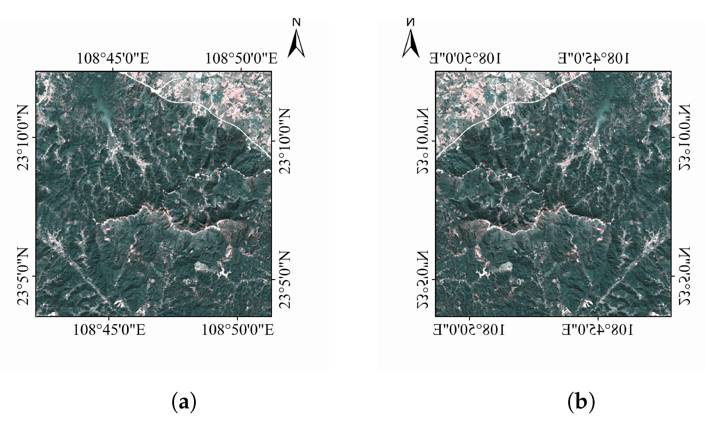
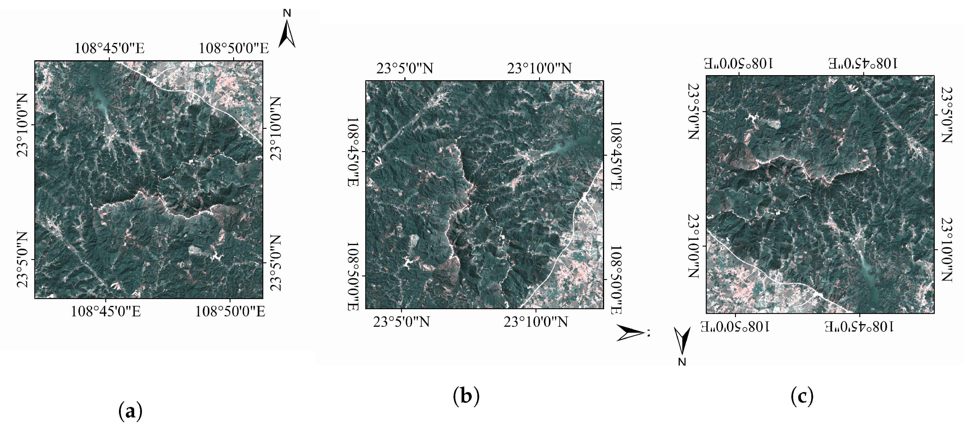
| LC81250442015104LGN01 | 125/44 | 14 April 2015 | 0.75% | 23.19 N, 108.9 E |
| LC81250442018304LGN00 | 125/44 | 31 October 2018 | 0.02% | 23.19 N, 108.9 E |
| Models | OA (%) | KC | Precision | Recall | F-Measure | IoU |
|---|---|---|---|---|---|---|
| FCSC 1 | 99.42 | 0.7774 | 0.8779 | 0.7023 | 0.7803 | 0.6398 |
| FCSD 2 | 99.16 | 0.7636 | 0.6474 | 0.9431 | 0.7677 | 0.6230 |
| FCGD 3 | 99.11 | 0.5823 | 0.9311 | 0.4277 | 0.5861 | 0.4145 |
| FCDD 4 | 99.51 | 0.8255 | 0.8565 | 0.8013 | 0.8280 | 0.7064 |
| Row | Site Center |
|---|---|
| A | 222830N, 1093530E |
| B | 254500N, 1193430E |
| C | 231030N, 1091500E |
| D | 221600N, 1093230E |
| Models | OA(%) | KC | Precision | Recall | F-Measure | IoU |
|---|---|---|---|---|---|---|
| FCSC 1 | 99.33 | 0.6229 | 0.5202 | 0.7862 | 0.6261 | 0.4557 |
| FCSD 2 | 99.57 | 0.6426 | 0.7741 | 0.5524 | 0.6447 | 0.4757 |
| FCGD 3 | 99.17 | 0.5814 | 0.4543 | 0.8223 | 0.5852 | 0.4137 |
| FCDD 4 | 99.76 | 0.8169 | 0.8805 | 0.7640 | 0.8181 | 0.6923 |
| Row | Site Center |
|---|---|
| A | 233600N, 1091030E |
| B | 225630N, 1080900E |
| C | 240000N, 1083715E |
| D | 232515N, 1091315E |
| E | 230130N, 1081245E |
Publisher’s Note: MDPI stays neutral with regard to jurisdictional claims in published maps and institutional affiliations. |
© 2022 by the authors. Licensee MDPI, Basel, Switzerland. This article is an open access article distributed under the terms and conditions of the Creative Commons Attribution (CC BY) license (https://creativecommons.org/licenses/by/4.0/).
Share and Cite
Guo, Y.; Long, T.; Jiao, W.; Zhang, X.; He, G.; Wang, W.; Peng, Y.; Xiao, H. Siamese Detail Difference and Self-Inverse Network for Forest Cover Change Extraction Based on Landsat 8 OLI Satellite Images. Remote Sens. 2022, 14, 627. https://doi.org/10.3390/rs14030627
Guo Y, Long T, Jiao W, Zhang X, He G, Wang W, Peng Y, Xiao H. Siamese Detail Difference and Self-Inverse Network for Forest Cover Change Extraction Based on Landsat 8 OLI Satellite Images. Remote Sensing. 2022; 14(3):627. https://doi.org/10.3390/rs14030627
Chicago/Turabian StyleGuo, Yantao, Tengfei Long, Weili Jiao, Xiaomei Zhang, Guojin He, Wei Wang, Yan Peng, and Han Xiao. 2022. "Siamese Detail Difference and Self-Inverse Network for Forest Cover Change Extraction Based on Landsat 8 OLI Satellite Images" Remote Sensing 14, no. 3: 627. https://doi.org/10.3390/rs14030627
APA StyleGuo, Y., Long, T., Jiao, W., Zhang, X., He, G., Wang, W., Peng, Y., & Xiao, H. (2022). Siamese Detail Difference and Self-Inverse Network for Forest Cover Change Extraction Based on Landsat 8 OLI Satellite Images. Remote Sensing, 14(3), 627. https://doi.org/10.3390/rs14030627