Article

Spatial Representativeness of Gross Primary Productivity from Carbon Flux Sites in the Heihe River Basin, China

1
Research Institute of Forest Resource Information Techniques, Chinese Academy of Forestry, Beijing 100091, China
2
Key Laboratory of Forestry Remote Sensing and Information System, National Forestry and Grassland Administration, Beijing 100091, China
3
State Key Laboratory of Remote Sensing Science, Jointly Sponsored by Beijing Normal University and Institute of Remote Sensing and Digital Earth of Chinese Academy of Sciences, Beijing 100875, China
4
Beijing Engineering Research Center for Global Land Remote Sensing Products, Faculty of Geographical Science, Institute of Remote Sensing Science and Engineering, Beijing Normal University, Beijing 100875, China
*
Author to whom correspondence should be addressed.
These authors contributed equally to this work.
Remote Sens. 2021, 13(24), 5016; https://doi.org/10.3390/rs13245016
Submission received: 10 November 2021 / Revised: 3 December 2021 / Accepted: 9 December 2021 / Published: 10 December 2021

Abstract

:
Studying the spatial representativeness of carbon flux measurement data for typical land cover types can provide important information for benchmarking Earth system models and validating multiple-scale remote sensing products. In our study, daily gross primary productivity (GPP) was firstly derived from eddy covariance observation systems and seasonal variations in field GPP were analyzed at nine flux tower sites for typical land cover types in the Heihe River Basin, China. Then, the real-time footprint distance and climate footprint distance of the field GPP were obtained by using a footprint source area model. Lastly, multiple-scale GPP products were validated at footprint scale, and the impacts (measurement height, surface roughness and turbulent state of the atmosphere) on the footprint distance of field GPP were analyzed. The results of this paper demonstrated that climate footprint distances ranged from about 500 m to 1500 m for different land cover types in the Heihe River Basin. The accuracy was higher when validating MODIS GPP products at footprint scale (R2 = 0.56, RMSE = 3.07 g C m−2 d−1) than at field scale (R2 = 0.51, RMSE = 3.34 g C m−2 d−1), and the same situation occurred in the validation of high-resolution downscaled GPP (R2 = 0.85, RMSE = 1.34 g C m−2 d−1 when validated at footprint scale; R2 = 0.82, RMSE = 1.47 g C m−2 d−1 when validated at field scale). The results of this study provide information about the footprints of field GPP for typical land cover types in arid and semi-arid areas in Northwestern China, and reveal that precision may be higher when validating multiple-scale remote sensing GPP products at the footprint scale than at the field scale.

1. Introduction

Gross primary productivity (GPP) is a fundamental variable in assessing controls on carbon dynamics because it varies with soil water availability, incident solar radiation, temperature, vegetation composition and nutrient availability [1,2]. Therefore, GPP is important in studying terrestrial vegetation carbon cycling and climate change [3]. GPP can be observed using eddy covariance systems at flux towers, which quantify the carbon exchange. However, the observed data can only reflect the carbon exchange to the extent to which the measurement taken in a spatial–temporal domain describes the actual environmental conditions in the space–temporal domain [4]. Remote sensing technology is a good way to simulate regional or global GPP, and to study carbon sources and carbon sinks; however, there is a scale difference between the remote sensing data and footprint of ground-observed GPP. In this context, studying the representativeness of the observed GPP from flux towers, and ways to match ground GPP and satellite-derived GPP is important in validating ecosystem models and remote sensing products. To summarize, the issue of spatial-temporal representativeness is of great significance in model–data benchmarking and remote sensing products’ validation [5].
Several studies have been conducted to analyze flux network-to-region representativeness, i.e., to analyze if the measured data from flux towers reflect the carbon flux in a region. For example, Villarreal et al. [6] analyzed the representativeness of the eddy covariance sites of AmeriFlux based on the ecosystem functional types categories represented by each network. Villarreal and Vargas [7] assessed the representativeness of registered FLUXNET sites across Latin America using GPP and evapotranspiration. Pallandt et al. [8] compared the environmental conditions observed at the tower locations and those within the larger Arctic domain, and mapped the representativeness of these eddy covariance network. Other studies have focused on analysis of the point-to-area representativeness [9], i.e., to what extent do measurements taken at the carbon flux tower reflect the carbon exchange around the measurement instruments. Over the last two decades, a number of footprint models have been proposed to simulate the source area for eddy covariance observations, such as the simple analytical footprint model based on Eulerian coordinates for scalar concentration (SAFE-C) [10], the flux source area model (FSAM) [11,12], the Hsieh model [13], and the Horst–Weil model [14]. Studies of the representativeness of flux tower data for different land cover types have also been conducted. For example, Järvi et al. [15] analyzed the sensitivity of the vertical fluxes at a single measurement point, and estimated the systematic uncertainty of eddy covariance flux measurements in annual cumulative values due to missing data for an urban area based on two towers. Kim et al. [16] analyzed the spatial representativeness of the source area for the vegetation characteristics (density variation and magnitude) within the surrounding area of a flux tower in a mixed forest. Rana et al. [17] studied the representativeness of observed carbon flux data in a Mediterranean urban area with equipment setup restrictions. Chu et al. [4] examined the land cover composition and vegetation characteristics in flux footprints and target areas across AmeriFlux sites, and analyzed the potential biases as a consequence of the footprint-to-target-area mismatch.
With the implementation of the Heihe Watershed Allied Telemetry Experiment Research (HiWATER) in the Heihe River Basin in Northwestern China, many algorithms have been developed and several remote sensing products have been generated in this area [18,19,20,21]. However, it is difficult to verify the accuracy of the proposed models and to validate multiple-scale remote sensing products due to the inadequacy of the footprint information for the carbon flux towers. Challenges still exist in interpreting and incorporating footprint information into these Earth system models due to the lack of footprint information for carbon flux sites [22,23]. Besides, the biases and uncertainty are still not clear when validating these Earth system models and multiple-scale remote sensing products due to a lack of footprint information and because most flux tower sites are located in more-or-less heterogeneous landscapes. In this context, studying the representativeness of the carbon flux data for typical land cover types in the Heihe River Basin, is important for benchmarking these models and multiple-scale remote sensing products in arid and semi-arid areas, which cover more than one-third of China [24].
The aims of this paper were to study the spatial representativeness of field GPP for several typical land cover types in the Heihe River Basin in China, and to analyze the influence factors related to the footprint of field GPP. The results of this paper provide information about the footprint of field GPPs in arid and semi-arid areas in Northwestern China, and reveal a number of impact factors related to the footprint distances of GPP from field eddy covariance systems at flux tower sites in the Heihe River Basin, China.

2. Materials and Methods
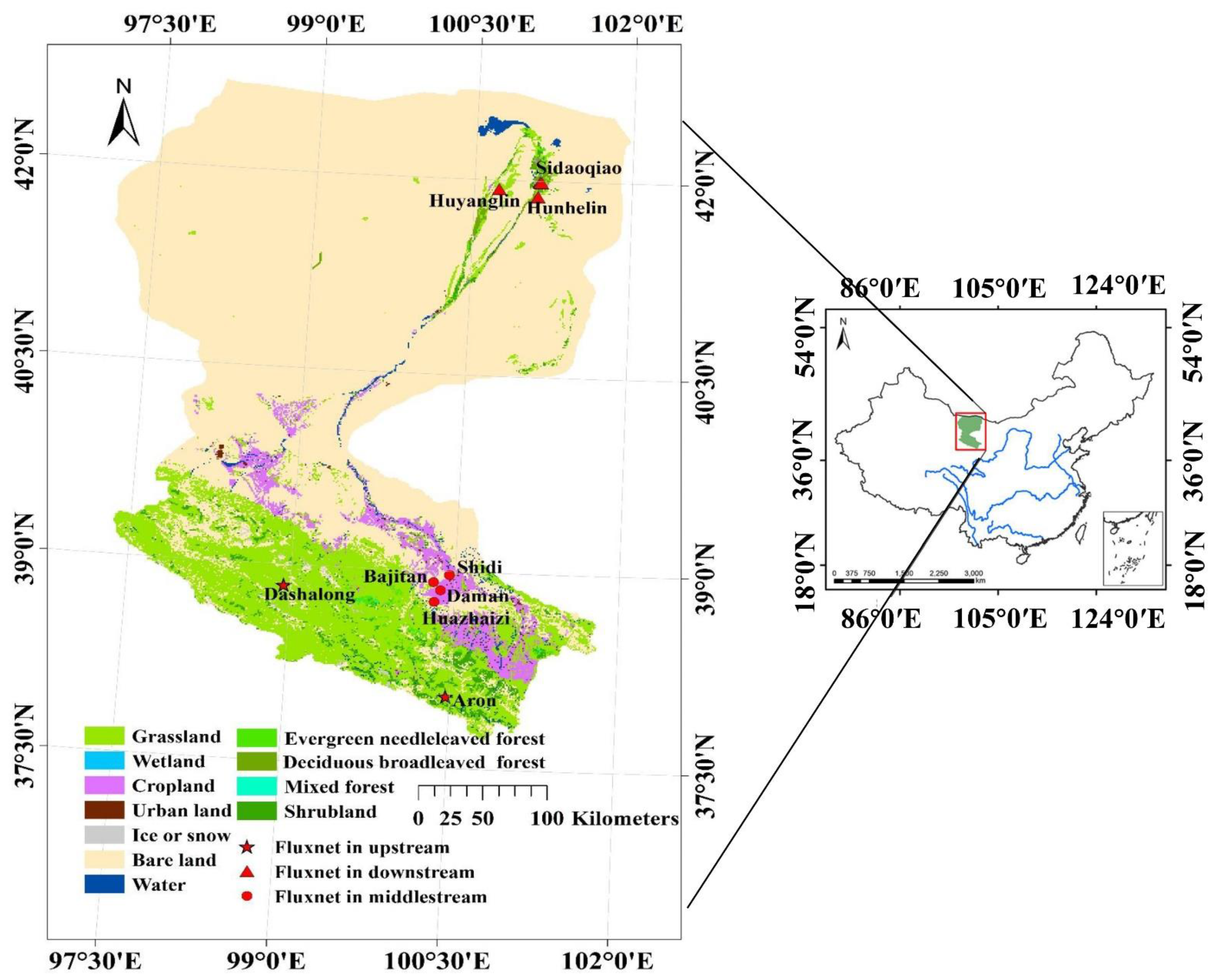
2.1. Study Area

The Heihe River Basin is located in Northwestern China (37°41′~42°42′N, 96°42′~102°00′E) (Figure 1). The elevation in this area ranges from 500 m in the Gobi in the northern areas to 5500 m in the mountains in the southern areas. The annual average temperature in the Heihe River Basin is about 6.0 °C to 8.0 °C, annual average precipitation is about 100 mm~400 mm [25], and annual average pan evaporation is about 1200 mm~1800 mm [26]. Croplands are mainly located in the upstream and middle stream in the Heihe River Basin with an area of about 8.5 × 10⁵ ha [27]. The Heihe River Basin is suitable for wheat, corn and Polish canola, with an annual output of 9.9 × 10⁵ tons [28]. The total area of forest is about 1.8 × 10⁵ ha [28], which is mainly located in the southwest of this region. The Heihe River Basin is a typical inland river basin in China, where water-stressed ecosystems are widely distributed, the eco-hydrological processes are complex, and the environment is more sensitive to climate change. Therefore, studying the representativeness of the observed carbon flux in this region is meaningful in revealing the applicability of Earth system models and validating remote sensing products in arid and semi-arid areas in Northwestern China.

2.2. Data and Data Processing

2.2.1. Carbon Flux Observed Data

The carbon flux data used in this paper were from the Multi-Scale Observation Experiment on Evapotranspiration for heterogeneous land surfaces, 2012 of the Heihe Watershed Allied Telemetry Experiment Research (HiWATER-MUSOEXE) [29,30,31]. Carbon flux data with a time interval of 30 min were obtained from nine flux tower sites from May to September in 2014, which is considered to be the growing season in the study area, and were used to study the spatial representativeness of GPP in this paper. The locations of these carbon flux towers are shown in Figure 1. The underlying surface types of the eddy covariance systems include Populus, crops (maize), grass, shrubs, wetland, Gobi and desert. The steps required to process the datasets included time delay corrections, density fluctuations, spectral loss, secondary coordinate rotation, sonic virtual temperature conversion, gaps filled, and the selection of high-quality carbon flux data [3,30,31,32,33,34,35]. The daily carbon flux was the summation of the 30-min data for one day. We calculated the difference in the estimated ecosystem respiration ( R e c o ) and observed net ecosystem carbon dioxide exchange (NEE) [36,37,38] as follows:
G P P = R e c o N E E

2.2.2. Meteorological Data

The air pressure, wind speed and direction, air temperature and humidity, precipitation, and radiation components (upward short-wave radiation, downward short-wave radiation, upward long-wave radiation, downward long-wave radiation) from May to September in 2014 were collected from meteorological stations at the flux towers to study the source area of field GPP. Half-hourly data were derived from the observed 10-min data. Missing data were filled-in by using the linear interpolation.

2.2.3. Land Cover Data

A 30 m land cover map was used to analyze the composition of land cover types on the footprint of field GPP in our study. This map was classified by using Chinese HJ-1 data [39]. Studies have shown that this land cover map has high accuracy (the overall classification accuracy of the map is 92.19%) [40,41].

2.2.4. Multi-Scale GPP Products
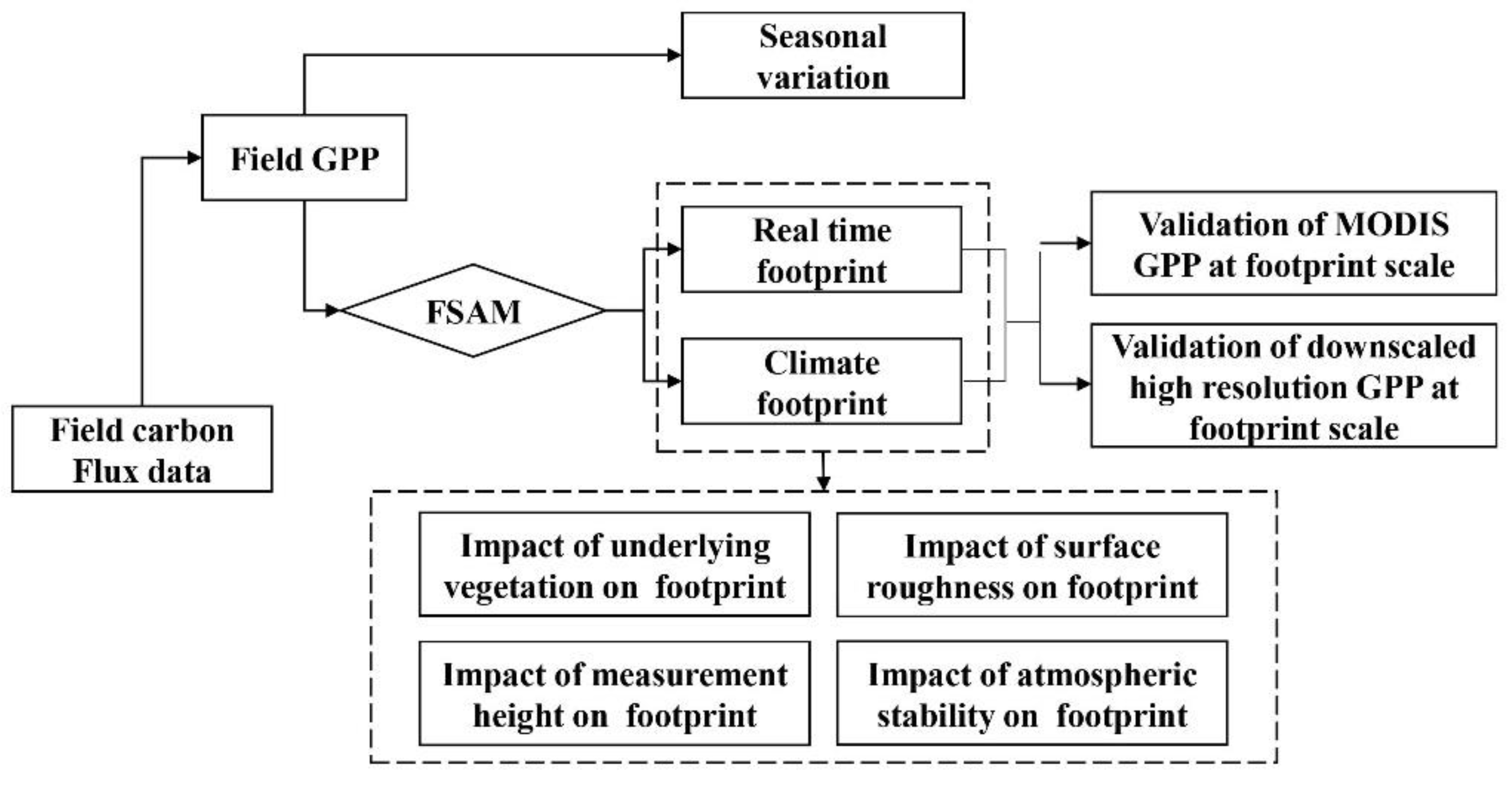
Moderate Resolution Imaging Spectroradiometer (MODIS) GPP products were used in this paper to compare the accuracy when validating field GPP at the footprint scale. MODIS GPP products (MOD17 A2H, Version 6) with a spatial resolution of 500 m and temporal resolution of 8 days were produced based on a light use efficiency model [42].
A 30 m GPP product with a temporal resolution of 8-day in the study area was also used in this paper to compare the accuracy when validating at field scale and at footprint scale. This GPP product was generated by using a downscaled model based on MODIS and Landsat data [43]. Specifically, fraction photosynthetically active radiation (FPAR) and leaf area index (LAI) with a spatial resolution of 30 m and a temporal resolution of 8 days were firstly generated from a downscaled method, and then 30 m GPP were obtained by using a light use efficiency model [43].

2.3. Methods

A flowchart of the process for analyzing the spatial representativeness of field GPP is shown in Figure 2. Firstly, the field GPP was derived from field carbon flux data and the seasonal trends of the GPP were analyzed. Then, a footprint source area model was used to reveal the real-time footprint and climate footprint at the flux tower sites for different land cover types. Lastly, MODIS GPP and downscaled high-resolution GPP products were validated at the footprint scale, and the impact of measurement height, surface roughness and atmospheric stability on the footprint distance of the field GPP were assessed, the composition of land cover types on the footprint of the field GPP was analyzed, and the uncertainly and limitations of this work were discussed.

2.3.1. Real-Time Footprint of Field GPP

The real-time flux footprint depends on the wind direction, measurement height, underlying ground surface characteristics and turbulent state of the atmosphere [44]. In this paper, the FSAM [11,12,45,46] was used to study the representativeness of field GPP for different land cover types in the Heihe River Basin. The FSAM is an analytical method model used to simulate the source area based on the K-theory and advection diffusion model. The carbon flux observed by this instrument can be described as [11,12]:
η = Q ( x , y ) f ( x , y , z m ) d x d y
where   η is the measured flux, Q ( x , y ) is the surface source distribution function, f ( x , y , z m ) is the footprint function, ( x , y , z m ) is the location of the instrument.
Based on the K theory, and a two-dimensional advection diffusion equation, the FSAM can obtain the source area under different contribution rates [11,12]:
P = 1 F u Ω p [ z 0 z m u ¯ ( z ) x C y ¯ ( x , z ) d z D y ( x , y ) ] d x d y
where P is the contribution rate, F u is the surface source–sink, Ω p is the flux source area, z m is the measurement height, z 0 is the surface roughness length, u ¯ is the mean wind speed profile, C y ¯ is the crosswind integrated concentration, and D y ( x , y ) is the crosswind integrated concentration distribution function. The key parameters used to run the FSAM, such as surface roughness length ( z 0 ), were obtained from experimental parameters [47,48]. The meteorological datasets used to run the FSAM were obtained from the automatic meteorological stations at the flux towers. The outputs of the FSAM include the length and location of the source area at different contribution rates.

2.3.2. Climate Footprint of Field GPP

The flux climate footprint, which is calculated by aggregating the real-time footprint, can be used to identify the spatial extents and temporal dynamics of the areas contributing to the observed fluxes at a tower site [44]. In this paper, a weighted footprint model was adopted to describe the climate footprint of field GPP [3]:
f c l i m a t o l o g y ( x , y , z m ) = i = 1 N f ( x , y , z m ) F l u x ( i ) F l u x ( i )
where f c l i m a t o l o g y ( x , y , z m ) is the climate footprint, i is the time intervals, N is the number of observed data in the time intervals, (x,y) is the locations, x and y is the direction of the up-wind and cross wind, z m is the measurement height, f ( x , y , z m ) is the real-time footprint, and F l u x ( i ) is the measured carbon flux.

2.3.3. Validation of Multiple GPP Products at Footprint Scale

Firstly, we directly compared the field GPP with MODIS GPP products and the downscaled GPP. Considering the co-registration errors between downscaled high resolution t images and field flux towers, the average GPP from a 3 × 3 pixels window around the flux towers was used when validating the downscaled GPP. Then, the weighted MODIS GPP or downscaled GPP in the footprint was compared with the measured data. Specifically, the weight of each pixel in the footprint was obtained according to the contribution rate to the total source area [3]:
R = f ( x , y , z m ) i i = 1 N f ( x , y , z m ) i × 100 %
where R is the weight, N is the total number of the pixels of GPP products in the footprint, and f ( x , y , z m ) i represents the footprint of i-th pixel.
The weighted average of the MODIS GPP or downscaled GPP was calculated and compared with measured GPP, and the determination coefficient (R2) and root mean square error (RMSE) were used to quantify the accuracy of GPP products.

3. Results

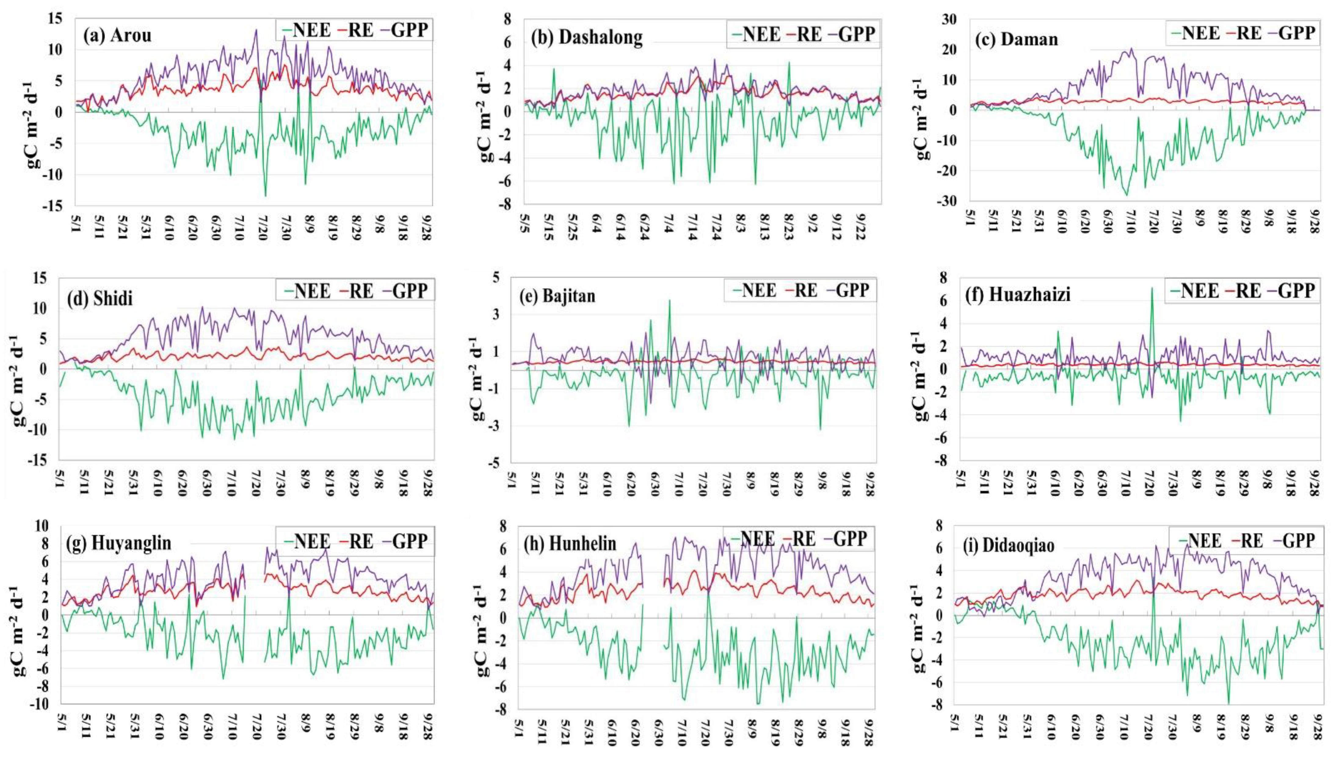
3.1. Seasonal Variation in Field GPP

We obtained time series for GPP, NEE and R e c o from May to September in 2014 (Figure 3). We found that GPP increased visibly from May to July, and then decreased from July to September in the study area. Generally, GPP was 20.60 g C m−2 d−1 in the peak in Daman (cropland, mainly maize), which was the highest among these land cover types. This was followed by Shidi (wetland), Huyanglin (deciduous broadleaved forest, DBF) and Hunhelin (mixed forest, MF), where the GPP was 10.28 g C m−2 d−1, 7.63 g C m−2 d−1, and 7.08 g C m−2 d−1, respectively. At Bajitan (Gobi) and Huazhaizi (desert), the GPP was 2.02 g C m−2 d−1 and 3.38 g C m−2 d−1, respectively, demonstrating that GPP was lowest in bare land among these land cover types. The average GPP in July was also highest in Daman (cropland), where the average GPP was 14.27 g C m−2 d−1. This was followed by Shidi (wetland), Huyanglin (DBF) and Hunhelin (MF), where the average GPP in July was 7.65 g C m−2 d−1, 5.38 g C m−2 d−1 and 5.47 g C m−2 d−1, respectively. The average GPP was 0.81 g C m−2 d−1 in Bajitan (Gobi), which was the lowest among these land cover types.

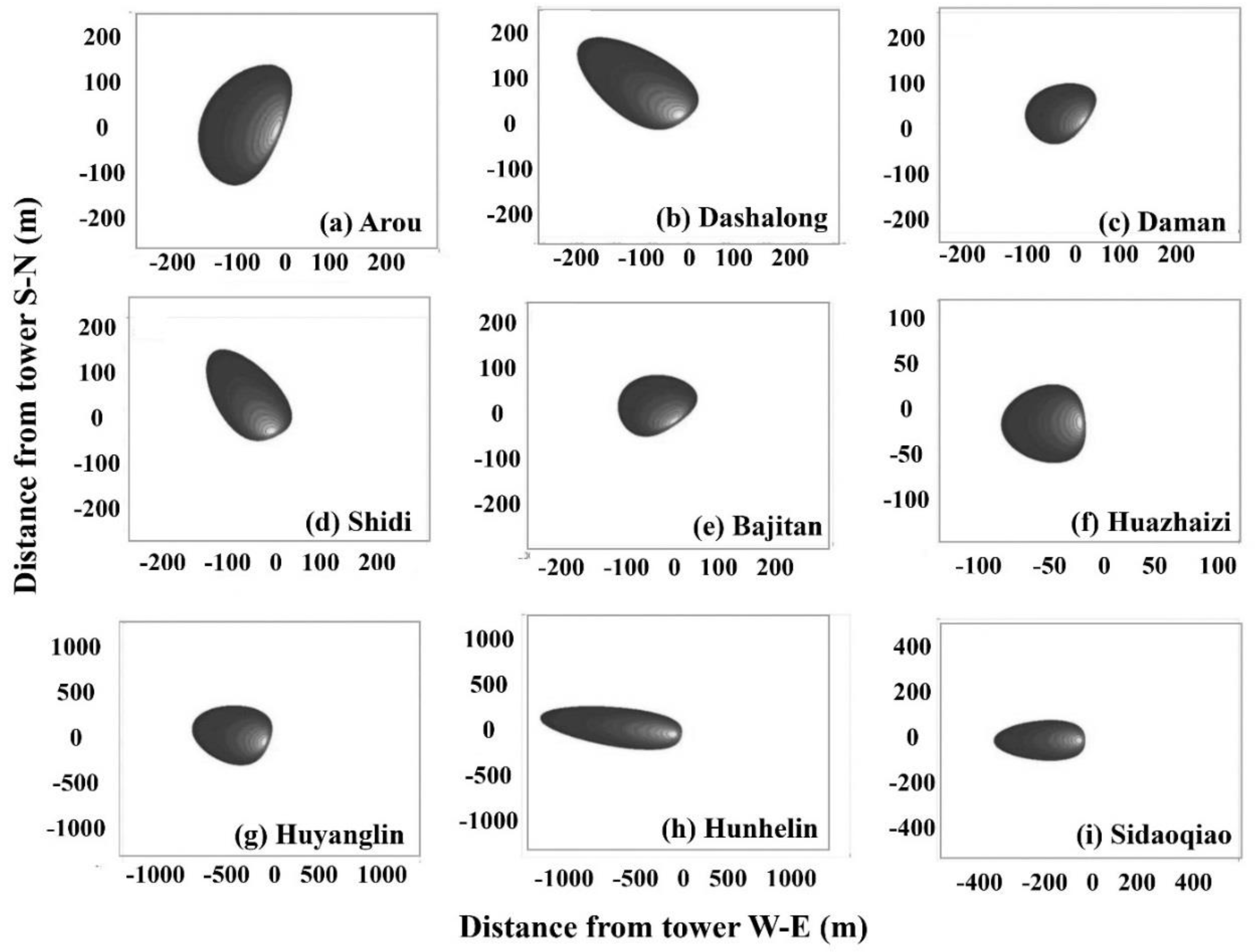
3.2. Footprint of Field GPP

3.2.1. Real-Time Footprint of Field GPP

A map of the real-time footprint of field GPP on 24 July, 2014, in which the atmosphere is relatively stable on a clear day, is shown in Figure 4. In general, the real-time footprint was consistent with the dominant wind directions, i.e., west and northwest wind. Footprint distances in the east to west direction were more than 500 m in Huyanglin (DBF) and Hunhelin (MF), demonstrating that footprint distances were the furthest in forest. In Sidaoqiao (shrub) and Shidi (wetland), the footprint distances were about 150~250 m. Footprint distances were less than 50 m in Huazhaizi (desert) and Bajitan (Gobi), which were the nearest among these land cover types. The wind direction and height of the instruments were the main factors influencing the real-time footprint, which will be discussed in Section 4.2.

3.2.2. Seasonal Variation in Climate Footprint of Field GPP

The monthly climate footprints of field GPP in the growing season in the study area are shown in Figure 5. The footprint distances were about 500 m to 1000 m at Arou (grass) in the northwest–southeast direction. Maximum footprint distances were about 600 m at Dashalong (grassland) in the northwest–southeast direction. In the middle stream area, the difference in the footprint was caused by the difference in the prevailing wind direction. The prevailing winds were west and northwest at Daman (cropland), northwest and southeast at Shidi (wetland), southwest at Huazhaizi (desert), north and southwest at Bajitan (Gobi). At Huyanglin (DBF) and Hunhelin (MF), the footprint distances were about 1200 m to 1500 m. At Sidaoqiao (shrub), the footprint distances were about 800 m to 1200 m.
We also found that iat Daman (cropland), Huazhaizi (desert) and Bajitan (Gobi), the monthly climate footprint varied significantly. The reasons may be that the surface roughness length changed with the state of growth of crops, and the atmospheric stability may change as these sites are located in the oasis regions. At Huazhaizi (desert) and Bajitan (Gobi), the land cover types were Gobi and desert. The wind speed was high and the wind direction varied, leading to varied footprints in these sites.

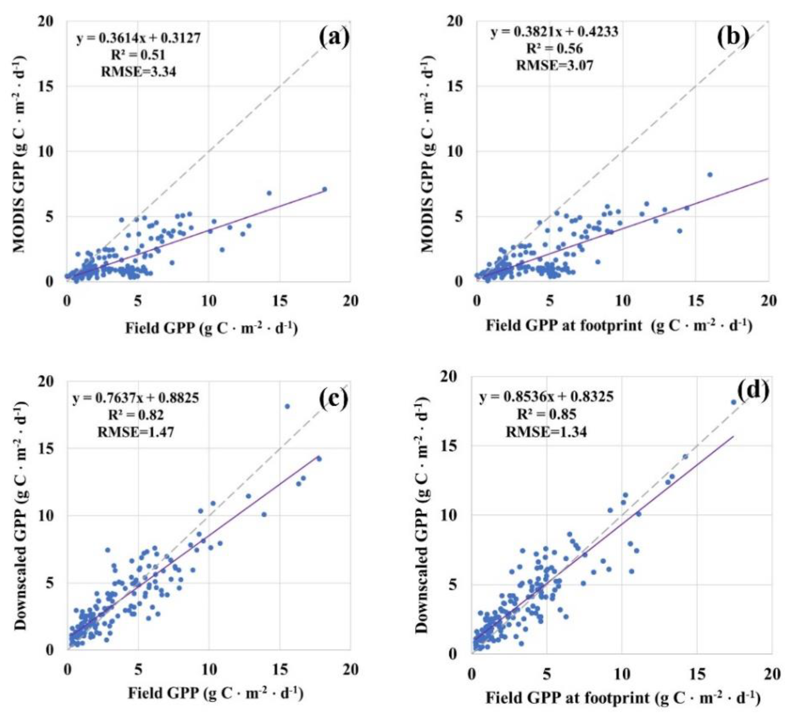
3.3. Comparison of Validation Multi-Scale GPP Products at Field Scale and at Footprint Scale

The MODIS GPP and downscaled GPP was validated at field scale and at footprint scale, as shown in Figure 6. Although studies have demonstrated that MODIS GPP was underestimated in the Heihe River Basin [49], we found that the accuracy of MODIS GPP was higher when validated at footprint scale (R2 = 0.56, RMSE = 3.07 g C m−2 d−1) than at field scale (R2 = 0.51, RMSE = 3.34 g C m−2 d−1). The same situation occurred in the validation of downscaled GPP. The precision of downscaled GPP was higher when validating in the footprint scale (R2 = 0.85, RMSE = 1.34 g C m−2 d−1) than validating GPP using field data directly (R2 = 0.82, RMSE = 1.47 g C m−2 d−1). This indicated that the representativeness of the observed carbon flux data provided some important information for the validation of remote sensing GPP products at different scales. This may be useful when taking into account the footprint of field data in the validation of multiple-scale remote sensing products [50,51].

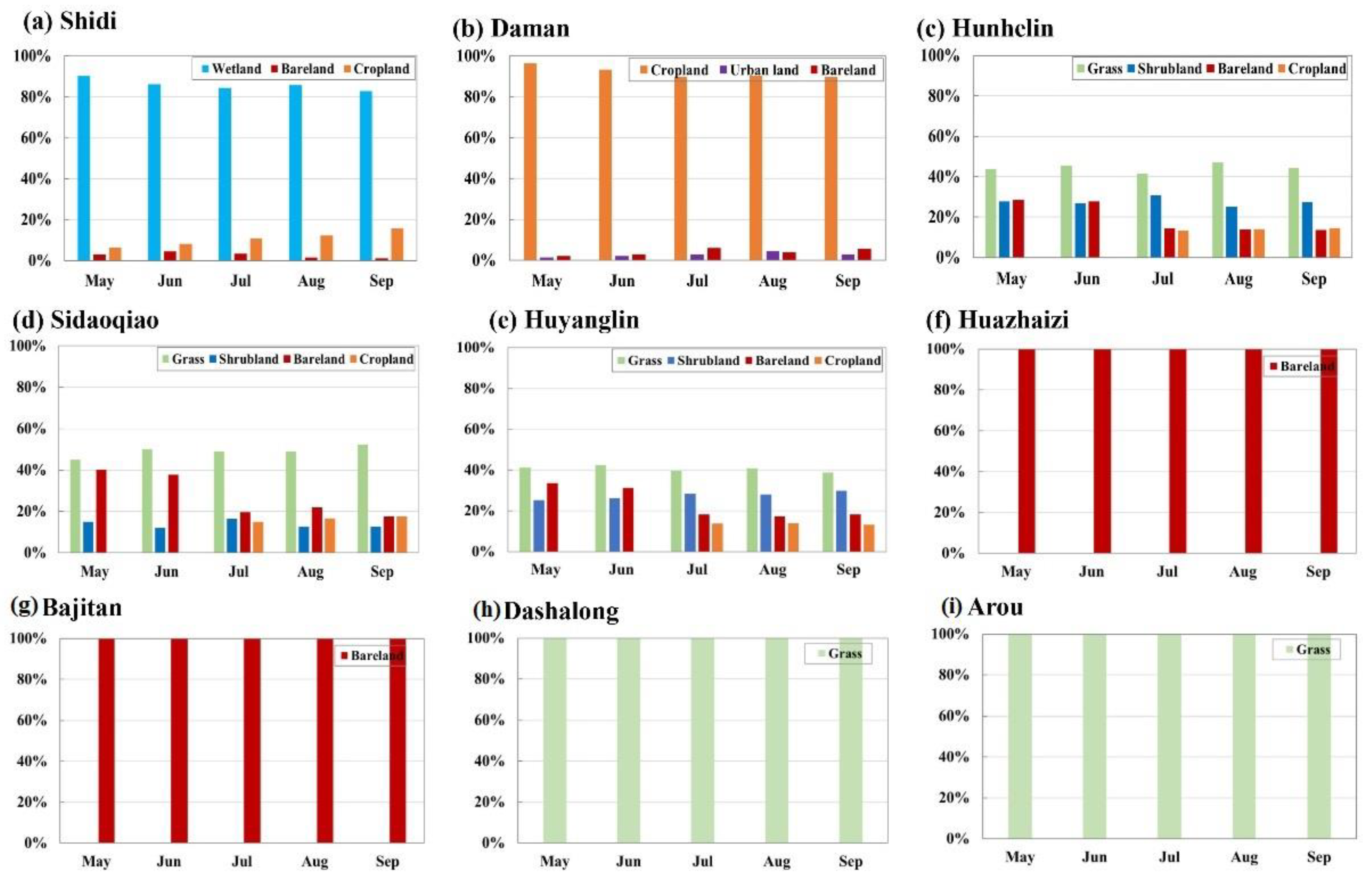
3.4. Land Cover Types in the Footprint

Studies have shown that the composition of the underlying vegetation and its spatial distribution around the eddy covariance observation systems certainly has an influence on the footprint [4,52,53]. The dominant land cover type within the footprints has the highest footprint-weighted percentage. To illustrate the contribution of different land cover types to the footprint, we analyzed the proportions of each land cover types in the footprint based on the 30 m land cover data, and the percentage of land cover types in the footprint is shown in Figure 7. The land cover type in the footprint was homogeneous at Huazhaizi, Bajitan, Dashalong and Arou. Specifically, bare land accounted for 100% of the footprint at Huazhaizi and Bajitan, grass land accounted for 100% in the footprint at Dashalong and Arou from May to September in 2014. However, multiple land cover types were located in the footprints of the other sites (Daman, Shidi, Huyanglin, Hunhelin, Sidaoqiao). The area of the dominant land cover type accounted for more than 90% of the footprint at Daman (cropland), and more than 80% at Shidi (wetland). At Hunhelin, Huyanglin and Sidaoqiao, the dominant land cover types only accounted for less than 50% of the footprint. This demonstrated that the underlying surface was related to the distance of the footprint.

3.5. Main Impact Factors of the Field GPP Footprint

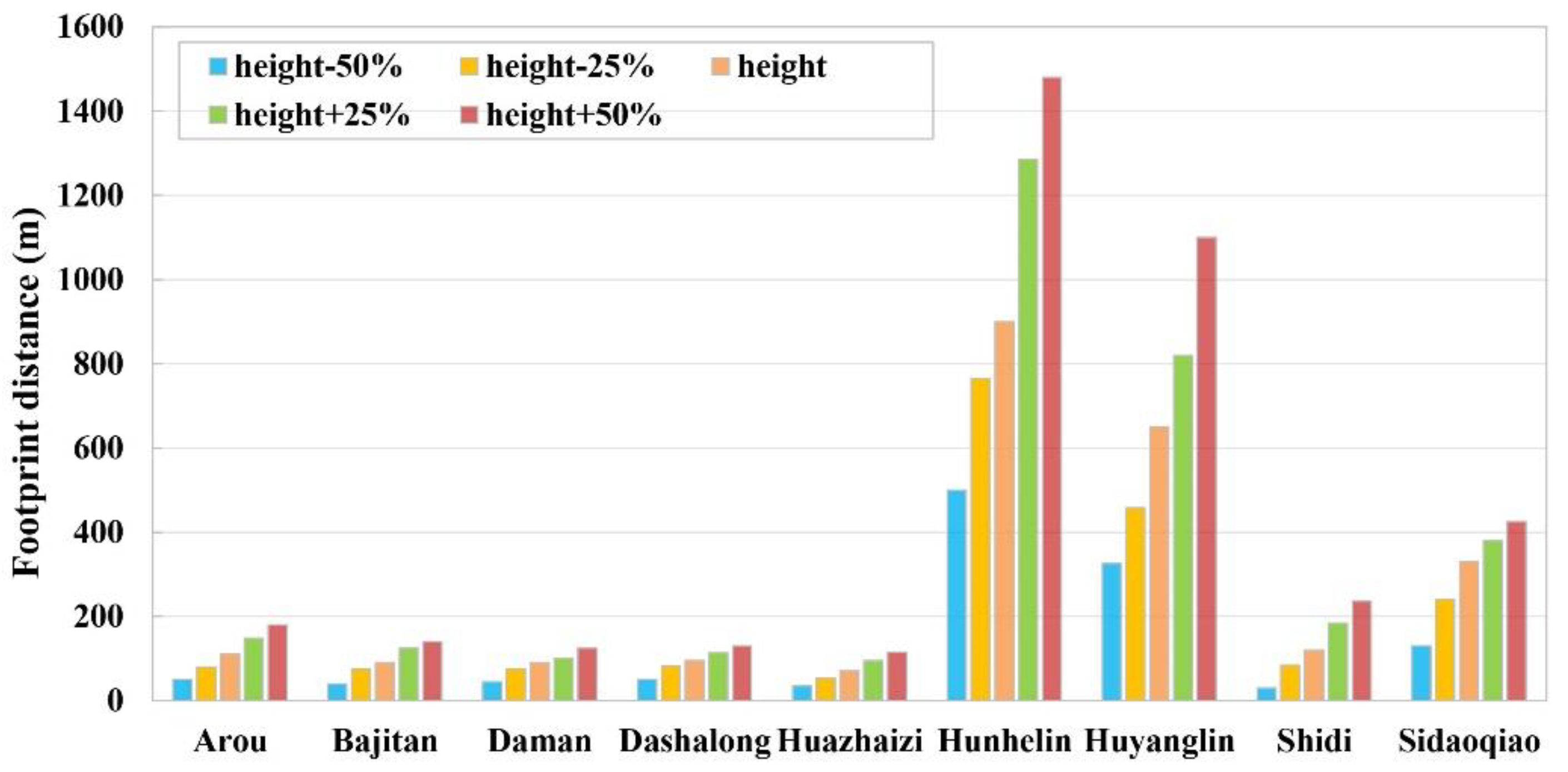
3.5.1. Influence of Measurement Height on Footprint of Field GPP

Measurement height was one of the main factors affecting the footprint distance of field GPP [44,54]. In general, the GPP footprint distance increased with the increase in the height of the eddy covariance systems. In the study area, the footprint distances were the furthest (more than 800 m) at the forest sites (Huyanglin and Hunhelin, where the measurement heights were also the highest (22.00 m). At Huazhaizi and Arou, the footprint distances (less than 200 m) were the nearest, and the measurement height were also the lowest (2.85 m at Huazhaizi, 3.50 m at Arou). In order to illustrate this, we simulated the footprint distance as the measurement height increased by 25% and 50% or decreased by 25% and 50%. As shown in Figure 8, the footprint distance decreased by 23.87%~30.2% when the measurement height decreased by 25%, and decreased by 43.90%~65.20% when the measurement height decreased 50%. The footprint distance increased by 27.72%~36.21% with a 25% increase in the height of the eddy covariance systems, and increased 56.51%~74.90% with a 50% increase in the measurement height.

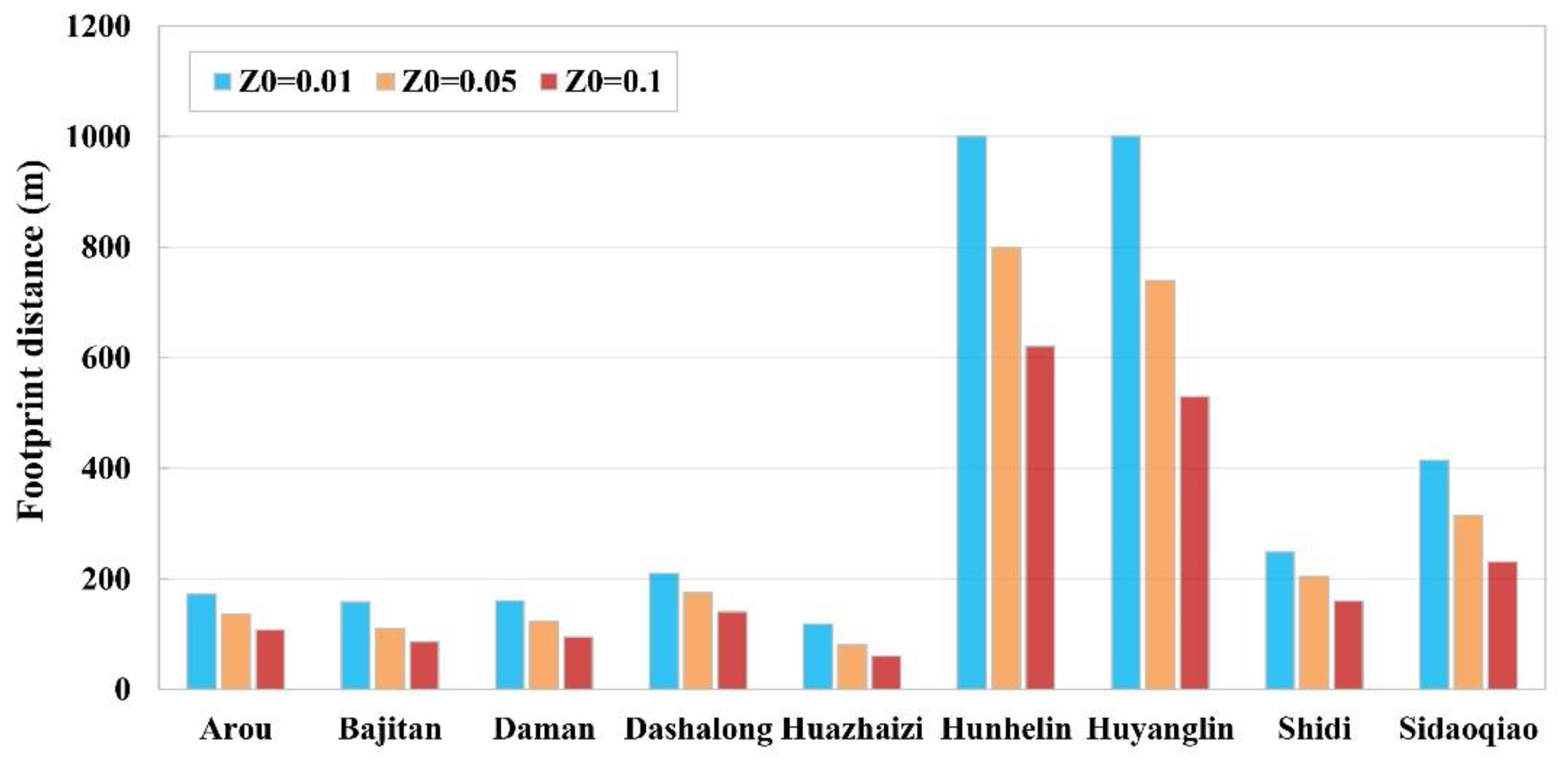
3.5.2. Influence of Surface Roughness on Footprint of Field GPP

In general, field GPP footprint distance decreased with the increase in surface roughness [38]. When the surface roughness increased from 0.01 m to 0.10 m, footprint distance of field GPP decreased about 33.3%~49.2% (footprint distances decreased more than 40% at Huazhaizi, Huyanglin, Bajitan, Sidaoqiao and Daman, and decreased about 33.0%~38% at Hunhelin, Arou, Shidi and Dashalong) (Figure 9).

3.5.3. Influence of Atmospheric Stability on Footprint of Field GPP

Field GPP footprint distance increased with the increase in atmospheric stability. In this paper, we analyzed the footprint distance when the atmospheric stability was at an unstable, stable and intermediate state (Figure 10). We found that the footprint distance became very small when the atmospheric state was unstable (footprint distances ranged from 15 m to 117 m). When the atmospheric stability was at the intermediate state, the footprint distance was further (footprint distances ranged from 96 m to 1122 m). When the atmospheric stability was at a stable state, the footprint distances were the furthest (footprint distances ranged from 154 m to 2468 m).

4. Discussion

4.1. Scale Mismatching between Satellte GPP and Ground Observed GPP

Studies have shown that GPP estimation from remote sensing are usually robust at most regional or global scales, but that the methods used from benchmarking and validation will impact the accuracy of the GPP estimation models [55]. The spatial resolution of GPP products from satellite observations range from a few hundred meters to tens of meters. Therefore, differences always exist due to the scale mismatch between the grid cells of remotely-sensed data and the scale of the ecological variable on the ground [56], which makes it difficult to directly evaluate remotely-sensed GPP using field carbon flux observations on the ground. Taking the footprint of ground-observed carbon flux into consideration is a good way to eliminate the scale difference between remote-sensing GPP and field-observed GPP. In this paper, the weighted MODIS GPP or downscaled GPP in the footprint were compared with the measured GPP, and higher precision was obtained when validating the multiple GPP products at footprint scale.
Several studies [3,57,58] demonstrated that upscaling the field GPP through machine learning methods was also a good way to make the field GPP comparable with remote sensing products. However, the uncertainties and error transfers in the upscaling process are still not very clear [59]. With the development of airborne and unmanned aerial vehicles (UAV) data, the gap between satellite data and field-measured carbon flux data may be filled, which may be helpful in satellite-derived GPP estimation and validation.

4.2. Limitations and Future Work

Uncertainties in the footprint calculation of observed GPP can result from the footprint models or errors in the input parameters [60]. Specifically, the key parameters to run FSAM, such as surface roughness length ( z 0 ), are related to the accuracy of footprint model. In this paper, the key parameters were obtained from the experimental parameter, which could bring some uncertainties in the estimation of the source area of the observed carbon flux data. Besides, footprints from nine flux tower sites covered most of the land cover types in the Heihe River Basin, but they are still insufficient to reflect all the land cover types in this region. In the future, we may conduct further research to assess the representativeness of the locations of the flux tower sites in this area. Furthermore, uncertainties related to the FSAM could also bring some errors. In the future, we may compare the difference between several footprint models, such as the flux footprint prediction (FFP) model [46] and the footprint symmetry index [4].

5. Conclusions

Studying the spatial representativeness of the field GPP for typical land cover types may provide important information for the measurement of carbon flux, as well as the validation of GPP at multiple scales. In this paper, field GPP was firstly derived from field eddy covariance systems. Seasonal trends and daily trends of field GPP were analyzed at nine flux tower sites over seven land cover types in the Heihe River Basin, China. Then, the real-time footprint distance and climate footprint distance of field GPP were described by using a footprint source area model. Lastly, MODIS GPP and downscaled GPP products were validated at the footprint scale, and the impacts (measurement height, surface roughness and atmospheric stability) on the footprint distance of field GPP were analyzed. The results of this paper provided information about the spatial representativeness of field GPP for the typical land cover types in the Heihe River Basin, and also demonstrated the influence factors on the footprint of field GPP in arid and semi-arid areas in Northwestern China.
Generally, significant diurnal and seasonal variation trends could be found at all land cover types, except bare land. Climate footprint distances ranged from about 500 m to 1500 m for different land cover types in the Heihe River Basin. When validating at footprint scale, the accuracy of the MODIS GPP and downscaled GPP was higher compared with validation at field scale. The field GPP footprint distance increased with the increase in the height of the eddy covariance systems and atmospheric stability, while the GPP footprint distance of field GPP decreased with the increase in surface roughness.

Author Contributions

Data curation, T.Y., Q.Z. and R.S.; writing—original draft preparation, T.Y. and Q.Z.; writing—review and editing, R.S.; visualization, T.Y. and Q.Z.; funding acquisition, R.S. All authors have read and agreed to the published version of the manuscript.

Funding

This research was funded by the National Key R&D Program of China (2017YFA0603002), and the Fundamental Research Funds of CAF (CAFYBB2021SY009).

Data Availability Statement

MODIS products data used in this study are available at https://modis.gsfc.nasa.gov/data/ (accessed on 9 December 2021), Meteorological and Land-cover data used in this study are available at http://data.casnw.net/portal/ (accessed on 9 December 2021).

Acknowledgments

Thanks for the reviewers’ suggestions and comments to improve this paper.

Conflicts of Interest

The authors declare no conflict of interest.

References

  1. Baldocchi, D.; Chu, H.; Reichstein, M. Inter-annual variability of net and gross ecosystem carbon fluxes: A review. Agric. For. Meteorol. 2018, 249, 520–533. [Google Scholar] [CrossRef] [Green Version]
  2. Biudes, M.S.; Vourlitis, G.L.; Velasque, M.C.S.; Machado, N.G.; de Morais Danelichen, V.H.; Pavão, V.M.; Arruda, P.H.Z.; de Souza Nogueira, J. Gross primary productivity of Brazilian Savanna (Cerrado) estimated by different remote sensing-based models. Agric. For. Meteorol. 2021, 307, 108456. [Google Scholar] [CrossRef]
  3. Yu, T.; Zhang, Q.; Sun, R. Comparison of machine learning methods to up-scale gross primary production. Remote Sens. 2021, 13, 2448. [Google Scholar] [CrossRef]
  4. Chu, H.; Luo, X.; Ouyang, Z.; Chan, W.; Dengel, S.; Biraud, S.C.; Torna, M.S.; Metzger, S.; Kumar, J.; Arain, M.A.; et al. Representativeness of eddy-covariance flux footprints for areas surrounding AmeriFlux sites. Agric. For. Meteorol. 2021, 301, 108350. [Google Scholar] [CrossRef]
  5. Durden, D.J.; Metzger, S.; Chu, H.; Collier, N.; Davis, K.J.; Desai, A.R.; Kumar, J.; Wieder, W.R.; Xu, M.; Hoffman, F.M. Automated integration of continentalscale observations in near-real time for simulation and analysis of biosphere–atmosphere interactions. In Driving Scientific and Engineering Discoveries through the Convergence of HPC, Big Data and AI; Springer: Berlin/Heidelberg, Germany, 2020. [Google Scholar]
  6. Villarreal, S.; Guevara, M.; Alcaraz-Segura, D.; Brunsell, N.A.; Hayes, D.; Loescher, H.W.; Vargas, R. Ecosystem functional diversity and the representativeness of environmental networks across the conterminous United States. Agric. For. Meteorol. 2018, 262, 423–433. [Google Scholar] [CrossRef]
  7. Villarreal, S.; Vargas, R. Representativeness of FLUXNET sites across Latin America. J. Geophys. Res. Biogeosci. 2021, 126, e2020JG006090. [Google Scholar] [CrossRef]
  8. Pallandt, M.; Kumar, J.; Mauritz, M.; Schuur, E.; Virkkala, A.M.; Celis, G.; Hoffman, F.; Göckede, M. Representativeness assessment of the pan-Arctic eddy-covariance site network, and optimized future enhancements. Biogeosci. Discuss. 2021, 133, 1–42. [Google Scholar]
  9. Schmid, H.P. Experimental design for flux measurements: Matching scales of observations and fluxes. Agric. For. Meteorol. 1997, 87, 179–200. [Google Scholar] [CrossRef]
  10. Chen, B.; Zhang, H.; Coops, N.C.; Fu, D.; Worthy, D.E.J.; Xu, G.; Black, T.A. Assessing scalar concentration footprint climatology and land surface impacts on tall-tower CO2, concentration measurements in the boreal forest of central Saskatchewan, Canada. Theor. Appl. Climatol. 2014, 118, 115–132. [Google Scholar] [CrossRef]
  11. Schmid, H.P. Source areas for scalars and scalar fluxes. Bound. Layer Meteorol. 1994, 67, 293–318. [Google Scholar] [CrossRef]
  12. Schmid, H.P.; Lloyd, C.R. Spatial representativeness and the location bias of flux footprints over inhomogeneous areas. Agric. For. Meteorol. 1999, 93, 195–209. [Google Scholar] [CrossRef]
  13. Hsieh, C.I.; Katul, G.; Chi, T.W. An approximate analytical model for footprint estimation of scalar fluxes in thermally stratified atmospheric flows. Adv. Water Rerour. 2000, 23, 765–772. [Google Scholar] [CrossRef]
  14. Horst, T.W.; Weil, J. Footprint estimation for scalar flux measurements in the atmospheric surface layer. Bound. Layer Meteorol. 1992, 59, 279–296. [Google Scholar] [CrossRef]
  15. Järvi, L.; Rannik, Ü.; Kokkonen, T.V.; Kurppa, M.; Karppinen, A.; Kouznetsov, R.D.; Pekka, R.; Timo, V.; Wood, C.R. Uncertainty of eddy covariance flux measurements over an urban area based on two towers. Atmos. Meas. Tech. 2018, 11, 5421–5438. [Google Scholar] [CrossRef] [Green Version]
  16. Kim, J.; Hwang, T.; Schaaf, C.L.; Kljun, N.; Munger, J.W. Seasonal variation of source contributions to eddy-covariance CO2 measurements in a mixed hardwood-conifer forest. Agric. For. Meteorol. 2018, 253, 71–83. [Google Scholar] [CrossRef]
  17. Rana, G.; Martinelli, N.; Famulari, D.; Pezzati, F.; Muschitiello, C.; Ferrara, R.M.M. Representativeness of carbon dioxide fluxes measured by eddy covariance over a mediterranean urban district with equipment setup restrictions. Atmosphere 2021, 12, 197. [Google Scholar] [CrossRef]
  18. Zhao, J.; Li, J.; Liu, Q.; Fan, W.; Zhong, B.; Wu, S.; Yang, L.; Zeng, Y.; Xu, B.; Yin, G. Leaf area index retrieval combining HJ1/CCD and Landsat8/OLI data in the Heihe River Basin, China. Remote Sens. 2015, 7, 6862–6885. [Google Scholar] [CrossRef] [Green Version]
  19. Fan, W.; Liu, Y.; Xu, X.; Chen, G.; Zhang, B. A new FAPAR analytical model based on the law of energy conservation: A case study in China. IEEE J. Sel. Top. Appl. Earth Obs. Remote Sens. 2014, 7, 3945–3955. [Google Scholar] [CrossRef]
  20. Li, X.; Liu, S.M.; Xiao, Q.; Ma, M.G.; Jin, R.; Che, T.; Wang, W.Z.; Hu, X.L.; Xu, Z.W.; Wen, J.G.; et al. A multiscale dataset for understanding complex eco-hydrological processes in a heterogeneous oasis system. Sci. Data 2017, 4, 170083. [Google Scholar] [CrossRef] [Green Version]
  21. Pan, X.; Li, X.; Yang, K.; He, J.; Zhang, Y.; Han, X. Comparison of downscaled precipitation data over a mountainous watershed: A case study in the Heihe River Basin. J. Hydrometeorol. 2014, 15, 1560–1574. [Google Scholar] [CrossRef]
  22. Griebel, A.; Metzen, D.; Pendall, E.; Burba, G.; Metzger, S. Generating spatially robust carbon budgets from flux tower observations. Geophys. Res. Lett. 2020, 47, e2019GL085942. [Google Scholar] [CrossRef]
  23. Stoy, P.C.; Mauder, M.; Foken, T.; Marcolla, B.; Boegh, E.; Ibrom, A.; Arain, M.A.; Arneth, A.; Aurela, M.; Bernhofer, C.; et al. A data-driven analysis of energy balance closure across FLUXNET research sites: The role of landscape scale heterogeneity. Agric. For. Meteorol. 2013, 171–172, 137–152. [Google Scholar] [CrossRef] [Green Version]
  24. Liu, H.; Tu, G.; Fu, C. Three-year variations of water, energy and CO2 fluxes of cropland and degraded grassland surfaces in a semi-arid area of Northeastern China. Adv. Atmos. Sci. 2008, 25, 1009–1020. [Google Scholar] [CrossRef] [Green Version]
  25. Cui, Y.; Song, L.; Fan, W. Generation of spatio-temporally continuous evapotranspiration and its components by coupling a two-source energy balance model and a deep neural network over the Heihe River Basin. J. Hydrol. 2021, 597, 126176. [Google Scholar] [CrossRef]
  26. Li, Y.; Huang, C.; Kustas, W.P.; Nieto, H.; Sun, L.; Hou, J. Evapotranspiration partitioning at field scales using TSEB and multi-satellite data fusion in the middle reaches of Heihe River Basin, Northwest China. Remote Sens. 2020, 12, 3223. [Google Scholar] [CrossRef]
  27. Gao, N.N.; Li, F.; Zeng, H.; Zheng, Y.R. The impact of human activities, natural factors and climate time-lag effects over 33 years in Heihe River Basin, China. Appl. Ecol. Environ. Res. 2021, 19, 1589–1606. [Google Scholar] [CrossRef]
  28. Liu, Q.; Niu, J.; Sivakumar, B.; Ding, R.; Li, S. Accessing future crop yield and crop water productivity over the Heihe River basin in northwest China under a changing climate. Geosci. Lett. 2021, 8, 2. [Google Scholar] [CrossRef]
  29. Li, X.; Cheng, G.; Liu, S.; Xiao, Q.; Ma, M.; Jin, R.; Che, T.; Liu, Q.; Wang, W.; Qi, Y.; et al. Heihe watershed allied telemetry experimental research (hiwater): Scientific objectives and experimental design. Bull. Am. Meteorol. Soc. 2013, 94, 1145–1160. [Google Scholar] [CrossRef]
  30. Liu, S.M.; Xu, Z.W.; Wang, W.; Jia, Z.Z.; Zhu, M.J.; Bai, J.; Wang, J.M. A comparison of eddy-covariance and large aper-ture scintillometer measurements with respect to the energy balance closure problem. Hydrol. Earth Syst. Sci. 2011, 15, 1291–1306. [Google Scholar] [CrossRef] [Green Version]
  31. Xu, Z.; Liu, S.; Li, X.; Shi, S.; Wang, J.; Zhu, Z.; Xu, T.; Wang, W.; Ma, M. Intercomparison of surface energy flux measurement systems used during the HiWATER-MUSOEXE. J. Geophys. Res. 2013, 118, 13140–13157. [Google Scholar] [CrossRef]
  32. Wilczak, J.M.; Oncley, S.P.; Stage, S.A. Sonic anemometer tilt correction algorithms. Bound. Layer Meteorol. 2001, 99, 127–150. [Google Scholar] [CrossRef]
  33. Liu, S.; Xu, Z.; Zhu, Z.; Jia, Z.; Zhu, M. Measurements of evapotranspiration from eddy-covariance systems and large aperture scintillometers in the Hai River Basin, China. J. Hydrol. 2013, 487, 24–38. [Google Scholar] [CrossRef]
  34. Papale, D.; Reichstein, M.; Aubinet, M.; Canfora, E.; Bernhofer, C.; Kutsch, W.; Longdoz, B.; Rambal, S.; Valentini, R.; Vesala, T.; et al. Towards a standardized processing of Net Ecosystem Exchange measured with eddy covariance technique: Algo-rithms and uncertainty estimation. Biogeosciences 2006, 3, 571–583. [Google Scholar] [CrossRef] [Green Version]
  35. Zhu, Z.; Sun, X.; Wen, X.; Zhou, Y.; Tian, J.; Yuan, G. Study on the processing method of nighttime CO2 eddy covariance flux data in ChinaFLUX. Sci. China Ser. D 2006, 49, 36–46. [Google Scholar] [CrossRef]
  36. Zhang, L.; Sun, R.; Xu, Z.; Qiao, C.; Jiang, G. Diurnal and seasonal variations in carbon dioxide exchange in ecosystems in the Zhangye oasis area, Northwest China. PLoS ONE 2015, 10, e0120660. [Google Scholar]
  37. Coops, N.C.; Black, T.A.; Jassal, R.P.S.; Trofymow, J.T.; Morgenstern, K. Comparison of MODIS, eddy covariance deter-mined and physiologically modelled gross primary production (GPP) in a Douglas-fir forest stand. Remote Sens. Environ. 2007, 107, 385–401. [Google Scholar] [CrossRef]
  38. Wang, H.; Saigusa, N.; Yamamoto, S.; Kondo, H.; Hirano, T.; Toriyama, A.; Fujinuma, Y. Net ecosystem CO2 exchange over a larch forest in Hokkaido, Japan. Atmos. Environ. 2004, 38, 7021–7032. [Google Scholar] [CrossRef]
  39. Landuse/Landcover Data of the Heihe River Basin. Available online: https://westdc.westgis.ac.cn (accessed on 5 October 2021).
  40. Zhong, B.; Yang, A.; Nie, A.; Yao, Y.; Zhang, H.; Wu, S.; Liu, Q. Finer resolution land-cover mapping using multiple classifiers and multisource remotely sensed data in the heihe river basin. IEEE J. Sel. Top. Appl. Earth Obs. Remote Sens. 2015, 8, 4973–4992. [Google Scholar] [CrossRef]
  41. Zhong, B.; Ma, P.; Nie, A.H.; Yang, A.X.; Yao, Y.J.; Lv, W.B.; Zhang, H.; Liu, Q.H. Land cover mapping using time series HJ-1/CCD data. Sci. China Earth Sci. 2014, 57, 1790–1799. [Google Scholar] [CrossRef]
  42. Heinsch, F.A.; Reeves, M.; Bowker, C.F. User’s Guide, GPP and NPP (MOD 17A2/A3) Products, NASA MODIS Land Algorithm. Available online: https://www.researchgate.net/publication/242118371_User\T1\textquoterights_guide_GPP_and_NPP_MOD17A2A3_products_NASA_MODIS_land_algorithm (accessed on 5 October 2021).
  43. Yu, T.; Sun, R.; Xiao, Z.; Zhang, Q.; Wang, J.; Liu, G. Generation of high resolution vegetation productivity from a downscaling method. Remote Sens. 2018, 10, 1748. [Google Scholar] [CrossRef] [Green Version]
  44. Schmid, H.P. Footprint modeling for vegetation atmosphere exchange studies: A review and perspective. Agric. For. Meteorol. 2002, 113, 159–183. [Google Scholar] [CrossRef]
  45. Kljun, N.; Kastner-Klein, P.; Fedorovich, E.; Rotach, M.W. Evaluation of Lagrangian footprint model using data from wind tunnel convective boundary layer. Agric. For. Meteorol. 2004, 127, 189–201. [Google Scholar] [CrossRef]
  46. Kljun, N.; Calanca, P.; Rotach, M.W.; Schmid, H.P. A simple two-dimensional parameterisation for Flux Footprint Predic-tion (FFP). Geosci. Model Dev. 2015, 8, 3695–3713. [Google Scholar] [CrossRef] [Green Version]
  47. He, H.; Zhang, L.; Gao, Y.; Ren, X.; Zhang, L.; Yu, G.; Wang, S. Regional representativeness assessment and improvement of eddy flux observations in China. Sci. Total Environ. 2015, 502, 688–698. [Google Scholar] [CrossRef]
  48. Yu, G.; Ren, W.; Chen, Z.; Zhang, L.; Wang, Q.; Wen, X.; He, N.; Zhang, L.; Fang, H.; Zhu, X.; et al. Construction and progress of Chinese terrestrial ecosystem carbon, nitrogen and water fluxes coordinated observation. J. Geogr. Sci. 2016, 26, 803–826. [Google Scholar] [CrossRef] [Green Version]
  49. Cui, T.; Wang, Y.; Sun, R.; Qiao, C.; Fan, W.; Jiang, G.; Hao, L.; Zhang, L. Estimating vegetation primary production in the Heihe River Basin of China with multi-source and multi-scale data. PLoS ONE 2016, 11, e0153971. [Google Scholar] [CrossRef] [Green Version]
  50. Turner, D.P.; Ollinger, S.; Smith, M.L.; Krankina, O.; Gregory, M. Scaling net primary production to a MODIS footprint in support of Earth observing system product validation. Int. J. Remote Sens. 2004, 25, 1961–1979. [Google Scholar] [CrossRef]
  51. Ramoelo, A.; Majozi, N.; Mathieu, R.; Jovanovic, N.; Nickless, A.; Dzikiti, S. Validation of global evapotranspiration product (MOD16) using flux tower data in the African savanna, South Africa. Remote Sens. 2014, 6, 7406–7423. [Google Scholar] [CrossRef] [Green Version]
  52. Battles, J.J.; Robards, T.; Das, A.; Waring, K.; Gilless, J.K.; Biging, G.; Schurr, F. Climate change impacts on forest growth and tree mortality: A data-driven modeling study in the mixedconifer forest of the Sierra Nevada, California. Clim. Chang. 2008, 87, 193–213. [Google Scholar] [CrossRef]
  53. Foley, J.A.; DeFries, R.; Asner, G.P.; Barford, C.; Bonan, G.; Carpenter, S.R.; Chapin, F.S.; Coe, M.T.; Daily, G.C.; Gibbs, H.K.; et al. Global Consequences of Land Use. Science 2005, 309, 570–574. [Google Scholar] [CrossRef] [PubMed] [Green Version]
  54. Chu, H.; Baldocchi, D.D.; Poindexter, C.; Abraha, M.; Desai, A.R.; Bohrer, G.; Arain, M.A.; Griffis, T.; Blanken, P.D.; O’Halloran, T.H.; et al. Temporal dynamics of aerodynamic canopy height derived from eddy covariance momentum flux data across North American Flux Networks. Geophys. Res. Lett. 2018, 45, 9275–9287. [Google Scholar] [CrossRef]
  55. Lees, K.J.; Khomik, M.; Quaife, T.; Clark, J.M.; Hill, T.; Klein, D.; Ritson, J.; Artz, R.R. Assessing the reliability of peatland GPP measurements by remote sensing: From plot to landscape scale. Sci. Total Environ. 2021, 766, 142613. [Google Scholar] [CrossRef] [PubMed]
  56. Xiao, J.; Chevallier, F.; Gomez, C.; Guanter, L.; Hicke, J.A.; Huete, A.R.; Ichii, K.; Ni, W.; Pang, Y.; Rahman, A.F.; et al. Remote sensing of the terrestrial carbon cycle: A review of advances over 50 years. Remote Sens. Environ. 2019, 233, 111383. [Google Scholar] [CrossRef]
  57. Duan, Z.; Yang, Y.; Zhou, S.; Gao, Z.; Zong, L.; Fan, S.; Yin, J. Estimating gross primary productivity (GPP) over rice–wheat-rotation croplands by using the random forest model and eddy covariance measurements: Upscaling and comparison with the MODIS product. Remote Sens. 2021, 13, 4229. [Google Scholar] [CrossRef]
  58. Huang, Y.; Nicholson, D.; Huang, B.; Cassar, N. Global estimates of marine gross primary production based on machine learning upscaling of field observations. Glob. Biogeochem. Cycles 2021, 35, e2020GB006718. [Google Scholar] [CrossRef]
  59. Virkkala, A.M.; Aalto, J.; Rogers, B.M.; Tagesson, T.; Treat, C.C.; Natali, S.M.; Watts, J.D.; Potter, S.; Lehtonen, A.; Mauritz, M.; et al. Statistical upscaling of ecosystem CO2 fluxes across the terrestrial tundra and boreal domain: Regional patterns and uncertainties. Glob. Chang. Biol. 2021, 27, 4040–4059. [Google Scholar] [CrossRef]
  60. Kormann, R.; Meixner, F. An analytical footprint model for non-neutral stratification. Bound. Layer Meteorol. 2001, 99, 207–224. [Google Scholar] [CrossRef]
Figure 1. Location of the Heihe River Basin and nine carbon flux observation stations.
Remotesensing 13 05016 g001
Figure 2. Flowchart for analyzing the spatial representativeness of field GPP. Real-time footprint and climate footprint were obtained using a flux source area model. MODIS GPP and downscaled high resolution GPP were validated at footprint scale. And the main impact factors of field GPP footprint were analyzed.
Remotesensing 13 05016 g002
Figure 3. Seasonal variation in GPP, respiration of ecosystem (RE) and net ecosystem carbon dioxide exchange (NEE) in the growing season.
Remotesensing 13 05016 g003
Figure 4. Real-time footprint of field GPP. The footprint displayed in this figure is from 24 July 2014. The gray level describes the contribution rate of the source area.
Remotesensing 13 05016 g004
Figure 5. Climate footprint of field GPP from May to September in 2014. The gray level describes the cumulative weight contribution to the footprint.
Remotesensing 13 05016 g005
Figure 6. Validation of MODIS GPP and downscaled GPP. (a) Validation of MODIS GPP at field scale; (b) validation of MODIS GPP at footprint scale; (c) validation of downscaled GPP at field scale; (d) validation of downscaled GPP at footprint scale.
Remotesensing 13 05016 g006
Figure 7. Area ratio of land cover types in the footprint.
Remotesensing 13 05016 g007
Figure 8. Changes of field GPP footprint with the changes of measurement height.
Remotesensing 13 05016 g008
Figure 9. Changes in field GPP footprint with the changes in surface roughness.
Remotesensing 13 05016 g009
Figure 10. Changes in field GPP footprint with the changes in atmospheric stability.
Remotesensing 13 05016 g010
Publisher’s Note: MDPI stays neutral with regard to jurisdictional claims in published maps and institutional affiliations.

