Article

Retrieval of Fine-Grained PM2.5 Spatiotemporal Resolution Based on Multiple Machine Learning Models

1
School of Geographical Sciences, Nantong University, Nantong 226007, China
2
Department of Land Surveying and Geo-Informatics, The Hong Kong Polytechnic University, Hong Kong, China
*
Author to whom correspondence should be addressed.
Remote Sens. 2022, 14(3), 599; https://doi.org/10.3390/rs14030599
Submission received: 20 December 2021 / Revised: 21 January 2022 / Accepted: 24 January 2022 / Published: 26 January 2022

Abstract

:
Due to the country’s rapid economic growth, the problem of air pollution in China is becoming increasingly serious. In order to achieve a win-win situation for the environment and urban development, the government has issued many policies to strengthen environmental protection. PM2.5 is the primary particulate matter in air pollution, so an accurate estimation of PM2.5 distribution is of great significance. Although previous studies have attempted to retrieve PM2.5 using geostatistical or aerosol remote sensing retrieval methods, the current rough resolution and accuracy remain as limitations of such methods. This paper proposes a fine-grained spatiotemporal PM2.5 retrieval method that comprehensively considers various datasets, such as Landsat 8 satellite images, ground monitoring station data, and socio-economic data, to explore the applicability of different machine learning algorithms in PM2.5 retrieval. Six typical algorithms were used to train the multi-dimensional elements in a series of experiments. The characteristics of retrieval accuracy in different scenarios were clarified mainly according to the validation index, R2. The random forest algorithm was shown to have the best numerical and PM2.5-based air-quality-category accuracy, with a cross-validated R2 of 0.86 and a category retrieval accuracy of 0.83, while both maintained excellent retrieval accuracy and achieved a high spatiotemporal resolution. Based on this retrieval model, we evaluated the PM2.5 distribution characteristics and hourly variation in the sample area, as well as the functions of different input variables in the model. The PM2.5 retrieval method proposed in this paper provides a new model for fine-grained PM2.5 concentration estimation to determine the distribution laws of air pollutants and thereby specify more effective measures to realize the high-quality development of the city.

Graphical Abstract

1. Introduction

With the continuous advancement of urbanization and industrialization, the problem of air pollution has become increasingly serious. Ambient air pollution, mostly PM2.5, can cause severe harm to the regional ecological environment and human health [1,2]. For every 10% increase in PM2.5, lung cancer mortality increases by 15–27% [3]. Thus, monitoring PM2.5 concentrations is key to PM2.5 pollution research [4]. The spatiotemporal resolutions used in relevant studies on PM2.5 concentration estimation are mostly at the kilometer-scale [5,6] and daily-scale [7,8], which limits the dynamic assessment of air pollution and human exposure in local areas. Therefore, under the background of building an ecologically civilized society in a holistic way and pursuing sustainable urban development, PM2.5 retrieval with a high spatiotemporal resolution and a high level of accuracy is crucial.
The existing methods for estimating spatial concentrations of PM2.5 can be divided into two major types: One type of method uses interpolation according to the data of ground stations. However, the number of ground stations is limited, and the spatial distribution is discontinuous, which yields great uncertainty for the calculations of PM2.5 concentrations [9,10]. Therefore, only using the method of interpolation can cause a high level of deviation in the results [11]. Another method is to use remote sensing images to establish a PM2.5 retrieval model. Remote sensing images offer wide spatial coverage [12,13], which can effectively make up for the defects in the discontinuous spatial distribution of monitoring stations and improve retrieval accuracy [14]. Much work has been conducted on the data sources, estimation methods, and parameter settings in this field.
The earliest satellites used for the retrieval of PM2.5 were the Moderate-resolution Imaging SpectroRadiometer (MODIS) [10,15], the Multi-angle Imaging SpectroRadiometer [16,17], and the Visible Infrared Imaging Radiometer [18]. The aerosol optical depth (AOD) products provided by these satellites provide key physical quantities of atmospheric turbidity and can be used to estimate the amount of particulate matter in the atmosphere [19]. However, the spatial resolution of these products is at the kilometer level. This low spatial resolution makes it difficult to capture the PM2.5 concentration distributions on an urban block scale [20,21]. Moreover, satellite observations based on AOD often measure the whole atmospheric columns, making PM2.5 near the surface difficult to retrieve from the integrated quantities [22,23]. With the rising popularity of medium and high resolution remote sensing satellites, Landsat images have gradually been used to retrieve particulate matter concentrations [24,25]. Its 30 m spatial resolution is relatively high among the many satellites used for PM2.5 retrieval. Estimations with high spatial resolution and full spatial coverage can be realized by directly building a retrieval model between an image’s spectral value and the particle concentration [11,26]. Although the spatial resolution of retrieval results has been significantly improved, it remains difficult to describe the real-time distribution pattern of PM2.5 concentrations in polluted areas because the revisit period of Landsat is as long as 16 days [26]. Therefore, it is a challenge to obtain PM2.5 concentration distributions with high spatiotemporal resolutions using remote sensing images [27].
At the same time, the choice of modeling methods also has a great impact on the accuracy of PM2.5 retrieval. With the continuous improvement of computing power and algorithms, increasingly more machine learning methods have been used in PM2.5 estimations [28], such as multiple linear regression (MLR) [29], support vector regression (SVR) [30,31], random forest (RF) [10], and artificial neural network (ANN) [32]. Compared to traditional statistical methods, machine learning algorithms have a strong ability to describe nonlinear relationships with massive amounts of data, which can effectively reduce estimation errors [33]. Although machine learning algorithms have great advantages in PM2.5 estimation, most studies only focus on the application or improvement of a certain algorithm, so there remains a lack of applicability evaluations for different algorithms in the same scenario.
In addition, most related PM2.5 estimation models only take the meteorological conditions and remote sensing image characteristics as the influencing factors [34]. However, the PM2.5 distribution has complex spatiotemporal distribution characteristics and is easily affected by many other factors, such as urban functional zones [35], road vehicle flows [36], industrial layout, and department settings [37]. The different pollutant emission characteristics of these factors makes it necessary to input more elements into the PM2.5 retrieval model.
To solve the above problems, this paper proposes a retrieval model with a fine-grained spatiotemporal resolution that comprehensively considers Landsat 8 satellite images with a spatial resolution of 30 m, ground monitoring station data with a time resolution of 1 h, and a 1 km grid of socio-economic data. Landsat satellite images offer spatially continuous surface coverage information with a high spatial resolution and the meteorological and socio-economic data provide auxiliary variable information that affects PM2.5 concentration. These products were used together as the input parameters for the calculation of the retrieval model. On this basis, retrieval models based on MLR, k-nearest neighbor (kNN), SVR, regression tree (RT), RF, and back-propagation neural network (BPNN) were built, and the applicability of different algorithms was assessed. According to these analyses, PM2.5 concentration data of a high quality can be obtained, thus providing a reference for further epidemiological research on data dimension expansion and model selection.
The main innovations of this paper include the following:
  • A PM2.5 retrieval model that integrates high-resolution satellite images with meteorological and socio-economic variables was proposed. The retrieval results had a high level of accuracy while realizing a fine-grained spatiotemporal resolution.
  • Six typical machine learning algorithms were used to build a PM2.5 retrieval model. By comparing the results of these algorithms using quantitative validation indexes, the optimal algorithm recommendation for a specific application is given.
The rest of the paper is organized as follows: The study area, the dataset and the methodology are briefly introduced in Section 2. The experimental results are illustrated in Section 3 and the discussion and conclusion are presented in Section 4 and Section 5.

2. Materials and Methods
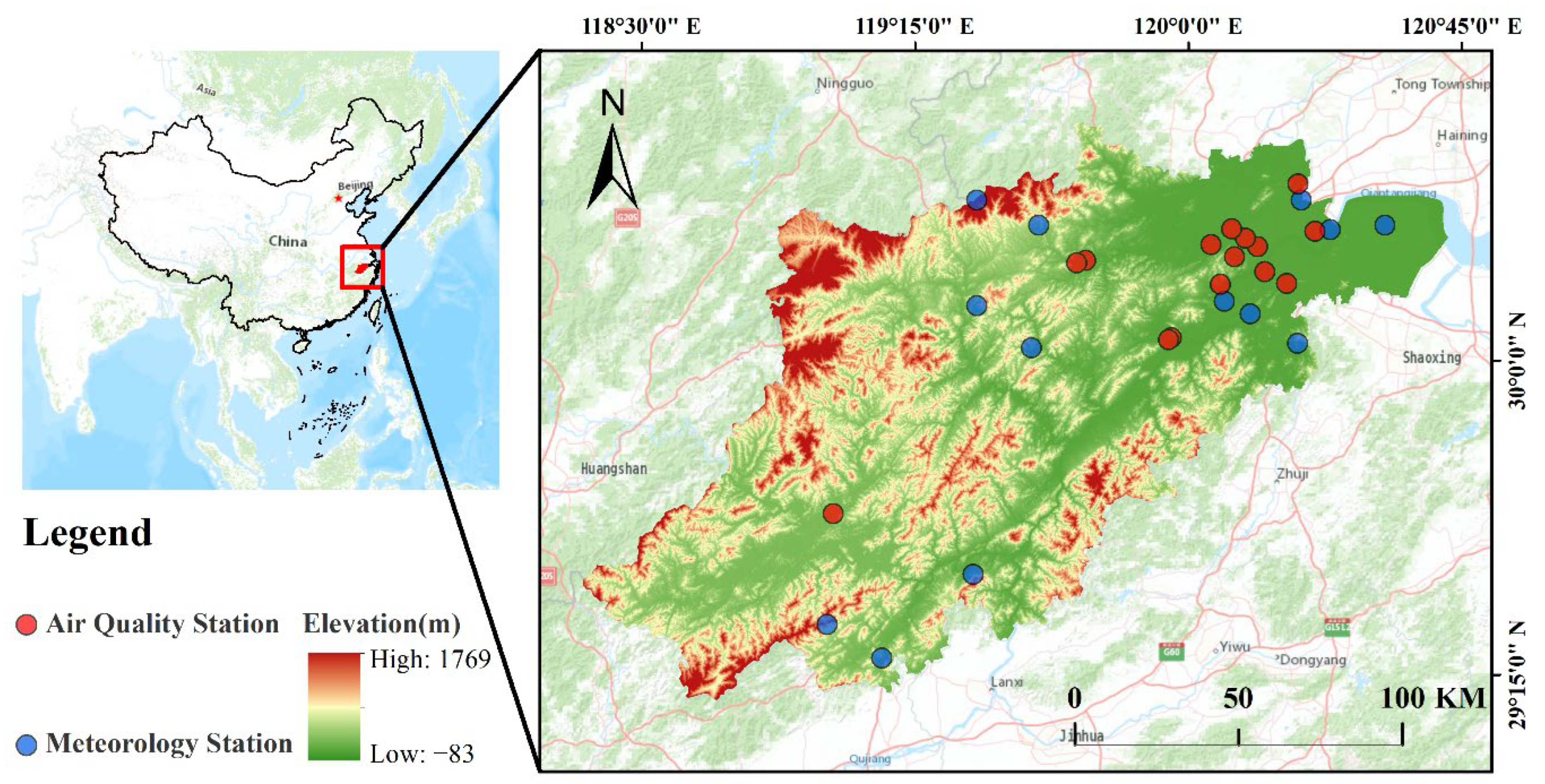
2.1. Study Area

Hangzhou, the capital city of Zhejiang, is an important central city in the Yangtze River Delta and a transportation hub in southeastern China (Figure 1). The total area of Hangzhou is around 16,853 km2, and the urbanization rate is 78.5%. Hangzhou is located in a subtropical monsoon climate area, with low terrain, a dense river network, and abundant rainfall. There are 15 air quality monitoring stations and 13 meteorological stations in the area, so the air quality and meteorological data are relatively sufficient.

2.2. Datasets and Data Preprocessing

2.2.1. Remote Sensing Image Data

In total, we used 53 Landsat 8 Operational Land Imager multispectral images with less cloud cover from the United States Geological Survey (USGS). These images were acquired from 22 May 2015, to 20 July 2019 and were preprocessed via radiometric calibration and Fast Line-of-sight Atmospheric Analysis of Hypercubes (FLAASH) atmospheric correction [38] on the PIE-Basic platform. These images feature 8 multispectral bands with a spatial resolution of 30 m and an image width of 185 × 170 km. The revisit period in China is 16 days.

2.2.2. Ground Monitoring Station Data

The hourly data of PM2.5 and weather conditions from 1 April 2015 to 31 August 2019, were provided, respectively, by the China National Environmental Monitoring Center (CNEMC) and the China Meteorological Administration (CMA). The meteorological elements included temperature (TEMP), precipitation (PREC), relative humidity (RH), and wind speed (WS).

2.2.3. Socio-Economic Data
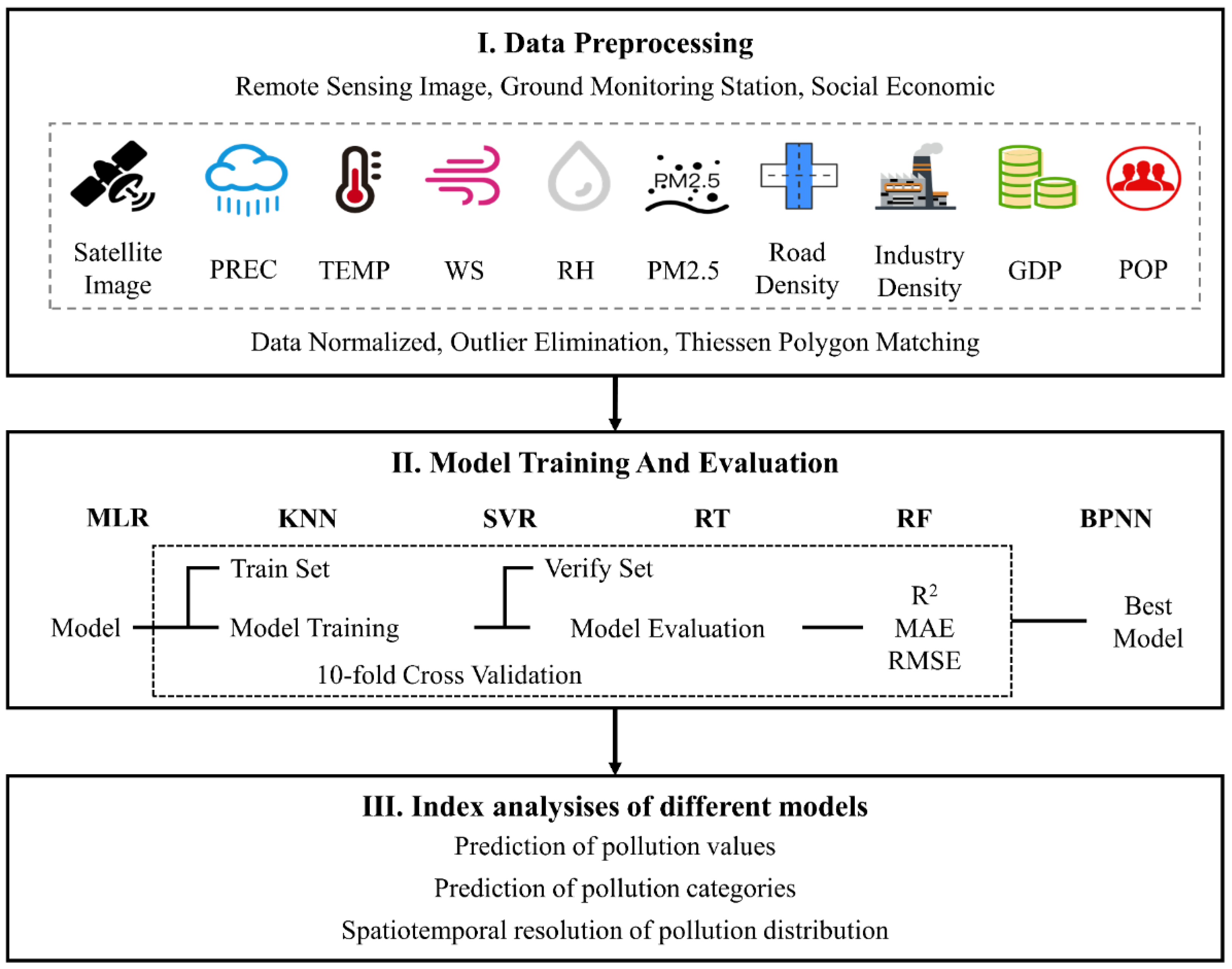
Other datasets included gross domestic product (GDP), population (POP), industry, and road networks. The GDP and POP data were obtained from the Resource and Environment Science and Data Center (RESDC). The industry data were acquired from Baidu Map’s Application Programming Interface using a web crawler, and the road network data were acquired from OpenStreetMap, which offers the latest road network data. These datasets were preprocessed by georeferencing, format conversion, and density calculations.
The categories, sources, and download links of the above multi-source datasets are provided in Table 1.

2.3. Methodology

Figure 2 illustrates the framework of this study and the details were as follows:
  • Preprocess the input data of the model. Because there were some data abnormalities, inconsistent data dimensions, and site-location mismatch problems in the input data, the data were first standardized, the outliers were removed, and Thiessen polygons were constructed to find the nearest-neighbor sites.
  • Build the retrieval model based on different machine learning algorithms. The MLR, kNN, SVR, RT, RF, and BPNN algorithms were used separately in this step to build the model. Validation index: MAE, RMSE, and R2, combined with the cross-validation method, were then used to evaluate the retrieval results.
  • Compare and analyze the indicators of different models. The pollution value and pollution categories of the retrieval results of different machine learning algorithms were compared, and the spatiotemporal resolution of the retrieval method in this study was compared with the resolutions presented in similar studies.

2.3.1. Data Integration

Different dimensions of datasets affect the comparability of indicators, so the raw data must be normalized. We used the min-max scaler method to linearly transform the raw data to a value between 0 and 1 to balance the data dimensions and, at the same time, speed up the model to find the global optimal hyper parameters. The formula was as follows:
Y = x x m i n x m a x x m i n
where x and Y , respectively, refer to the values before and after normalization, and x m i n and x m a x refer to the minimum and maximum values before normalization.
Because the locations of the meteorological stations and air quality monitoring stations are not co-located, the Thiessen polygon method was used to spatially associate the two groups of data. The Thiessen polygon, also known as the Voronoi diagram, is widely used to assess the traffic accessibility of traffic stations, schools, and shopping malls. Each polygon contains only one input point feature, and any position in the polygon is closer to its associated point than to any other point. According to Tobler’s first law of geography [39], the meteorological data from the air quality monitoring stations located in a certain Thiessen polygon can be expressed by the meteorological data of the associated points.

2.3.2. Machine Learning Algorithms

In this paper, the Python machine learning library scikit-learn was used for model building, and six typical machine learning algorithms (MLR, kNN, SVR, RT, RF, and BPNN) were used to retrieve the PM2.5 concentrations. The grid-search module of scikit-learn was employed for parameter optimization, and the parameter dictionary was used to adjust the candidate values of the hyper parameters to determine the best value. The final determination rule of hyper parameters was as follows: When the parameters are set in this way, the quantitative validation index of the model has the highest score. The validation index is introduced in the following Section 2.3.3. The main theory and hyper parameter values of the different models were as follows:
(1)
MLR
The multivariable linear regression model is an extension of the one-variable linear regression [40], in which there are often two or more independent variables that affect the dependent variable. For a given instance x = ( x 1 ; x 2 ; ; x d ) , the general form of the multivariable linear regression model is as follows:
f ( x )   = w 1 x 1 + w 2 x 2 + + w d x d + b
where d refers to the number of elements contained in   x , x i refers to the value of the i th attribute of   X , w refers to the regression coefficient, and b refers to the constant term.
(2)
kNN
The kNN algorithm uses a certain distance to determine the nearest k samples in the training set and then predicts other samples based on the k neighbors. As one of the most important parameters, k determines the neighborhood range of the training set, which will affect the estimation results of the kNN algorithm [41].
The distance between two sample points in feature space can reflect the degree of similarity between those points. The feature space of the kNN model is generally an n -dimensional vector space, and the distance between two points is usually measured by the Euclidean distance. The calculation process is shown in Formula (3). The final hyper parameters of this model were determined as follows: n_neighbors = 10, p = 2, and weights = distance.
d ( x , y ) = Σ k = 1 n ( x k y k ) 2
where x k and y k refer to the coordinates of point X and point Y , respectively, in the k th dimension, and n refers to the dimension of the data.
(3)
SVR
The SVR algorithm is an important application branch of support vector machines (SVM) [42]. In a given sample D = { ( x 1 , y 1 ) , ( x 2 , y 2 ) , , ( x n , y n ) , x i , y i R }   , the equation f ( x ) = ω T x + b   can be trained to make f ( x ) as close to y as possible. When measuring model accuracy, the prediction result is considered correct when the deviation between f ( x ) and y is not too large. Specifically, the tolerable deviation, ε , is set, and the loss is calculated only when the absolute value of the difference is greater than   ε , which can improve the robustness of the model. Specifically, the tolerable deviation ε is set to improve the robustness of the model. Only when the absolute value of the difference between f ( x ) and y   is greater than ε will the loss be calculated. The final hyper parameters of this model were determined as follows: C = 1.0, degree = 3, epsilon = 0.1, kernel = rbf, and max_iter = −1.
(4)
RT
The RT algorithm is a tree model that contains a root node, several internal nodes and several leaf nodes. When RT is used for regression, the input space x is divided into m units   R 1 , R 2 , , R M , which means that there will be at most M predicted values. The calculation used for minimizing the mean square error is shown in Formula (4). The final hyper parameters of this model were determined as follows: max_depth = 14, max_features = None, min_impurity_decrease = 0.0, min_impurity_split = None, min_samples_leaf = 1, and min_samples_split = 2.
Y = m i n 1 n Σ m = 1 M Σ x i R m 1 ( c m y i ) 2
where Y refers to the minimum mean square error, n refers to the number of samples, M refers to the number of divided input space, R m refers to the m th units after division, and c m refers to the predicted value of the m th leaf.
(5)
RF
The basic unit of RF is RT and it integrates multiple trees based on ensemble learning [43]. During the training stage, RF collects different sub-training datasets by bootstrap sampling and trains different decision trees based on these training datasets. During the prediction stage, RF averages the prediction values to obtain the final result, which prevents RF from falling into overfitting and tends to offer excellent anti-noise ability [43]. The final hyper parameters of this model were determined as follows: max_depth = 5, max_features = 19, min_impurity_split = None, min_samples_leaf = 10, and min_samples_split = 4.
(6)
BPNN
BPNN is a multi-layer feed-forward neural network characterized by signal-forward propagation and error-backward propagation. In BPNN, each neuron receives input signals from other neurons and transmits signals through weighted connections. The neurons sum these signals to obtain the total input value and compare it with the threshold value of the neurons. The output data of nodes can be calculated through nonlinear transformation using the transfer function. Moreover, nonlinear mapping of BPNN can solve the linear inseparable problem, greatly improving prediction accuracy [44]. The sigmoid transfer function is shown in Formula (5). The final hyper parameters of this model were determined as follows: activation = logistic, batch_size = auto, hidden_layer_sizes = (100, 100, 100, 100, and 100), learning_rate = constant, learning_rate_init = 0.001, and solver = sgd.
s i g m o i d ( z ) = 1 1 + e z
where z refers to a linear combination of the inputs in the network’s last layer.

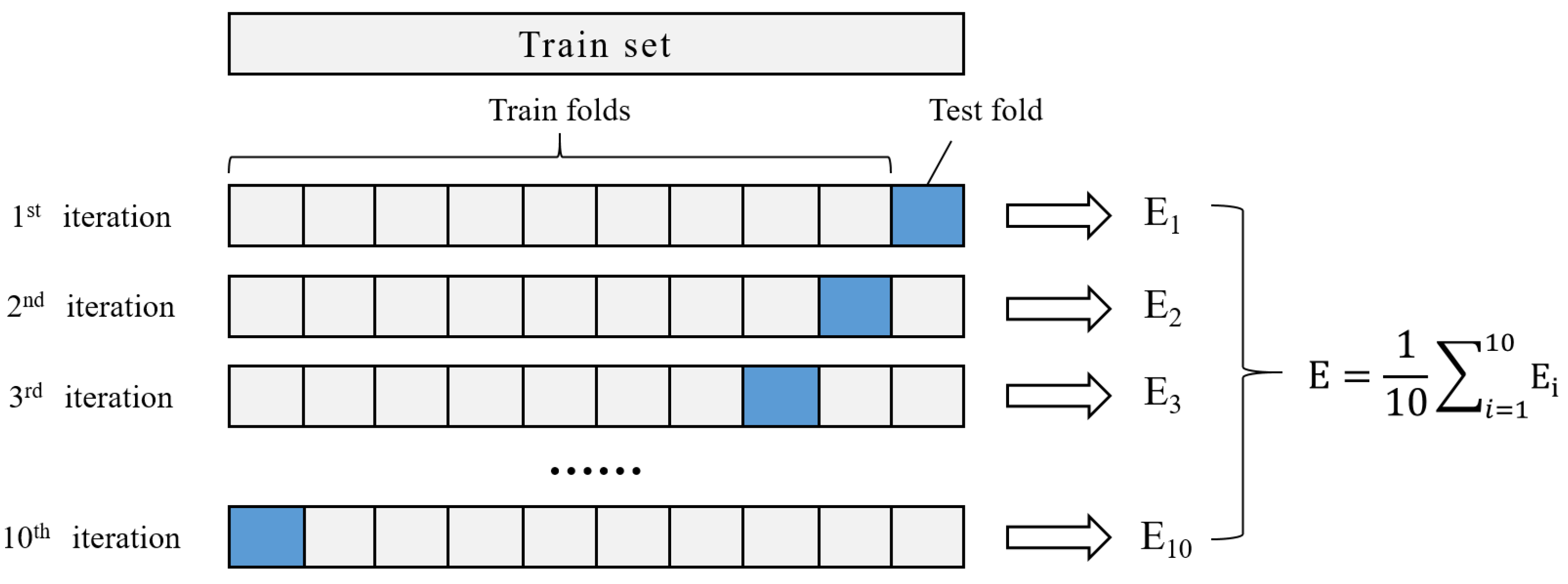
2.3.3. Model Validation

(1)
Validation method
K-fold cross-validation divides the dataset into a training set, a validation set and a test set. The three subsets are used to train the model, adjust the parameters and test the quality of the model under the current parameter settings. The schematic diagram of 10-fold cross-validation is shown in Figure 3, the dataset is divided randomly into 10 samples by non-repetitive sampling, then, 9 folds are used for training, and the remaining fold is used to test. This step is repeated 10 times to obtain 10 models and their evaluation results. Finally, the average result of these models is used to check the accuracy of the model. Overfitting is avoided by applying this method [45].
(2)
Validation Index
This paper uses the determination coefficient (R2), mean absolute error (MAE), and root mean square error (RMSE) as the validation indices of model accuracy. R2 represents the percentage of the fluctuation of y that can be described by the fluctuation of x , MAE presents the average absolute difference between the predicted value and the observed value, and RMSE presents how well the predicted value curve fits the observed value curve. The corresponding calculation formulas are as follows:
R 2 = i = 1 n ( y ^ i y ¯ ) 2 i = 1 n ( y i y ¯ ) 2
MAE = 1 n i = 1 n | y i y ^ i |
RMSE = 1 n i = 1 n ( y i y ^ i ) 2
where n refers to the number of data, y i refers to the i th observed value, y i ^ refers to the i th predicted value, y ¯ refers to the average of all observed values.

3. Results

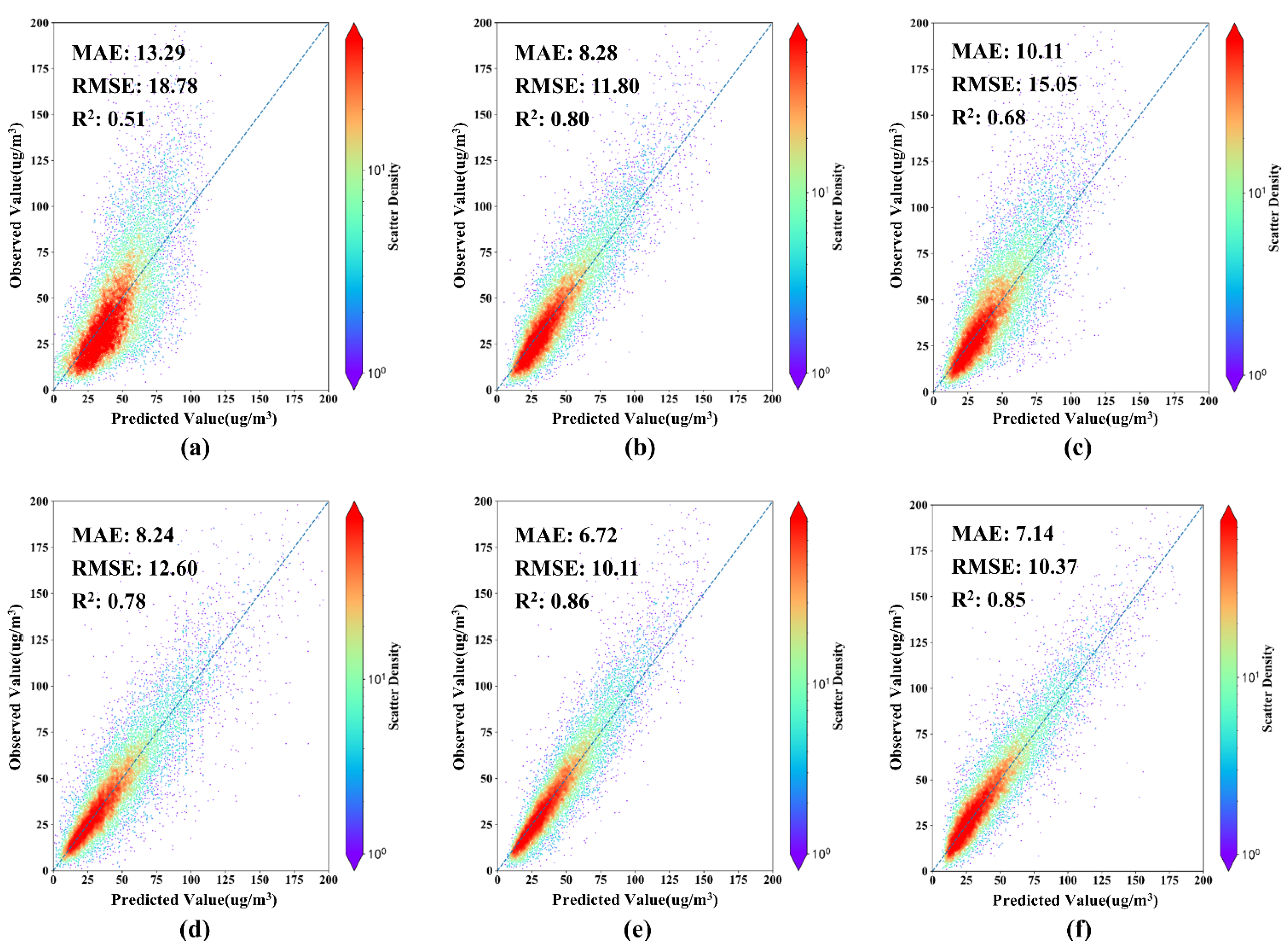
3.1. Analysis of PM2.5 Retrieval Results

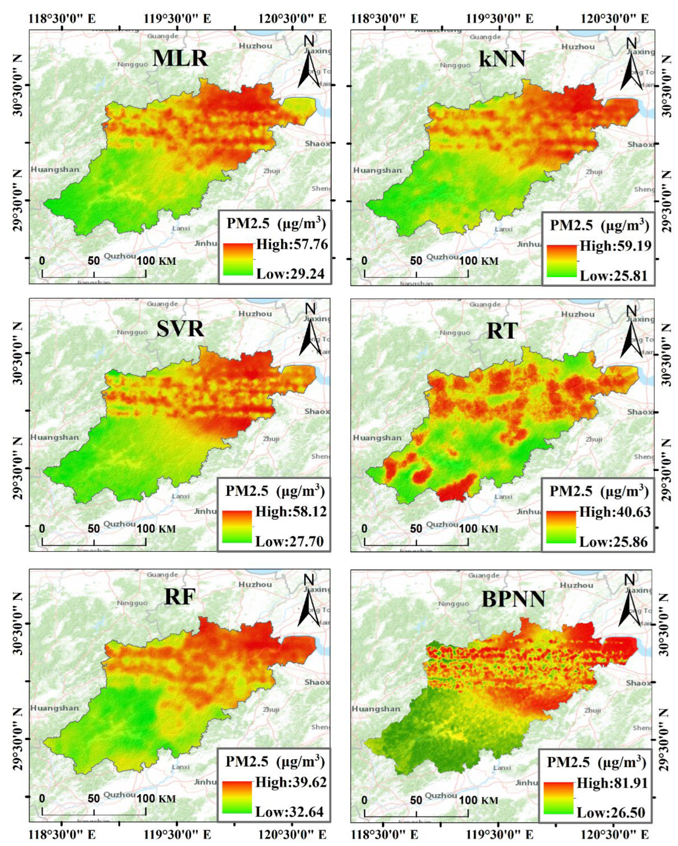
3.1.1. Prediction of the PM2.5 Concentration Distribution

Six machine learning algorithms were used to estimate the spatial distribution of PM2.5 at 11:00 on 15 April 2019 in Hangzhou, as shown in Figure 4. It can be found that except for the retrieval results of the RT model, which has several high PM2.5 areas in the southwest, the distribution estimated by the other models is consistent, which reflects the overall accuracy of the retrieval model. High values of PM2.5 are concentrated in the northeast, while low values are concentrated in the southwest. These results are closely related to the topography of Hangzhou. The southwest region is a hilly area and includes Tianmu Mountain, while the northeast region is the plain area of northern Zhejiang, which features low terrain, developed industry, dense population, and an active socio-economic life, which, again, indicates that PM2.5 concentrations are highly correlated with socio-economic factors.
The comparison of the results of the monitoring data and model fitting are shown in Figure 5. In general, when the concentration of PM2.5 is relatively low, the scatter distribution tends to be closer to the identity line. When the concentration exceeds 150 μg/m3, the prediction values of the MLR, kNN, SVR, and RF models are generally lower than the observed values, which indicates that these four models lack the ability to predict high PM2.5 concentration values. Although the BPNN model showed a better fitting effect in the high concentration area, this model still falsely estimated low values as high values.
The results of comparing the PM2.5 distribution eigenvalues calculated by the different models with the PM2.5 eigenvalues of the observed data are shown in Table 2. These results indicate that the RT model offers the best estimation of the maximum and minimum values of PM2.5, while the results of the MLR model were the worst, showing large deviations from the data distribution of the observed values. However, in calculating the average values of the data, the MLR model achieved the best results. In calculating the median of the data, the calculation result of the SVR model was the closest to the observed values. This result reflects the different strategies used by different algorithms to obtain the best and most optimized results. For example, the MLR algorithm employs a mean regression. The straight line corresponding to the regression equation will pass through the average center of the training data, so MLR will also have the best effect on the test set. This result shows that different algorithms should be used to solve different specific problems.
The scores of different validation indexes are shown in Table 3. By comparing the MAE, RMSE, and R2, we found that the MAE of all models were between 6.72 and 13.29, the RMSE were between 10.11 and 18.78, and the R2 were between 0.51 and 0.86, indicating that the feature selections and algorithm applications in this paper achieved good results. Here, the RF model performed best, with an R2 of up to 0.86, which means that the retrieval model could explain 86% of the training data. The R2 values of the kNN and BPNN models were above 0.8, but the R2 of the MLR model was relatively poor (0.51), indicating that the simple structure of the MLR model could not describe the complex nonlinear relationship between the PM2.5 concentration and the model elements. Estimations of the PM2.5 pollution value tended to improve the overall accuracy, while R2 best reflected the overall fit of the regression equation, so the RF model is more suitable for PM2.5 retrieval modeling.

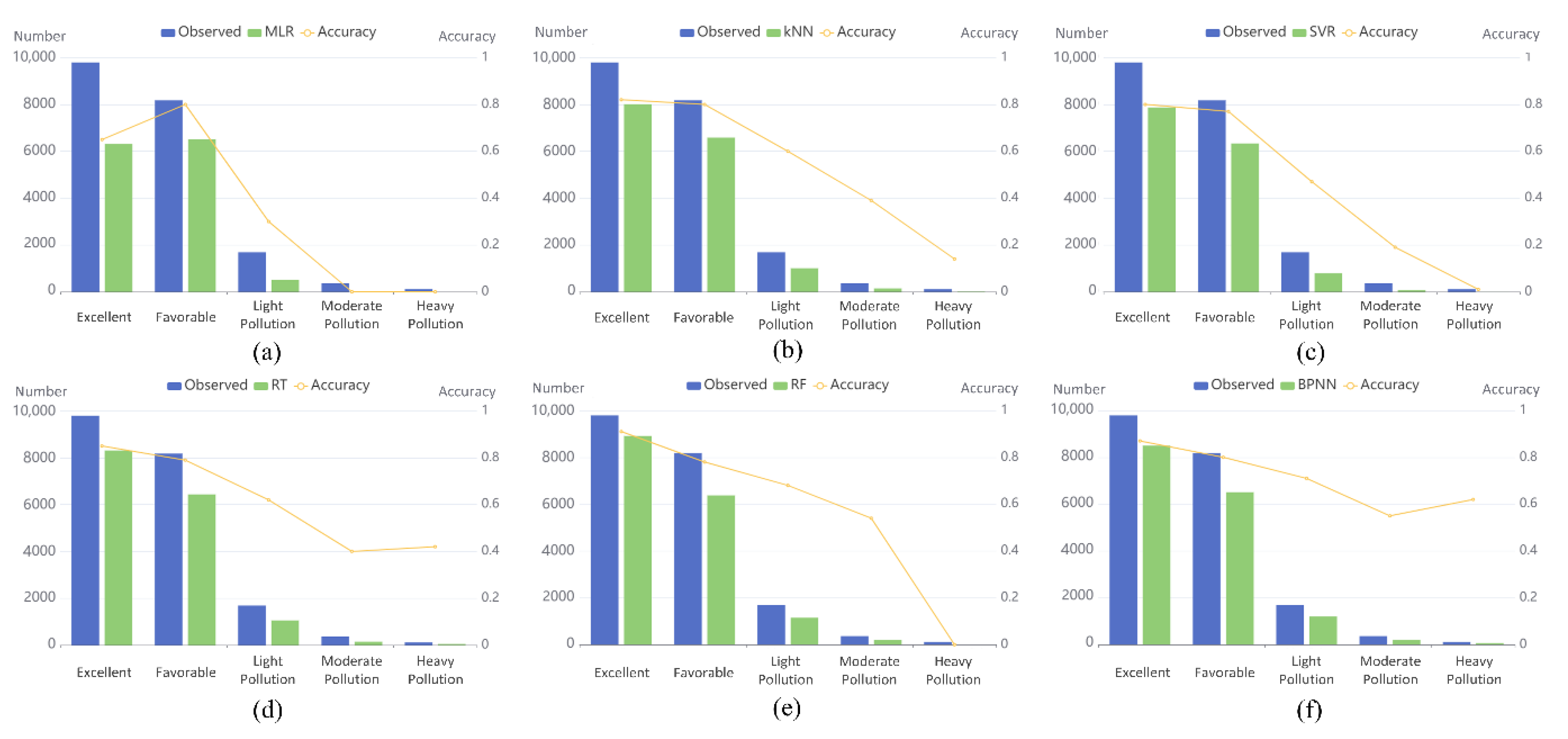
3.1.2. Prediction of PM2.5-Based Air Quality Categories

According to the air quality standards in China, daily PM2.5 concentrations are classified as “excellent” (0–35 μg/m3), “favorable” (35–75 μg/m3), “light pollution” (75–115 μg/m3), “moderate pollution” (115–150 μg/m3), “heavy pollution” (150–250 μg/m3), or “ultra-serious pollution” (>250 μg/m3). The performance of different machine learning algorithms in predicting PM2.5 pollution categories is shown in Figure 6.
The overall accuracy of the MLR, kNN, SVR, RT, RF, and BPNN algorithms in predicting the PM2.5 pollution categories were 66%, 78%, 75%, 79%, 83%, and 82%, respectively. Here, the RF algorithm had the highest accuracy. However, the RF accuracy for excellent, favorable, light pollution, moderate pollution, and heavy pollution was 91%, 78%, 68%, 54%, and 0%, respectively. These results indicate an overall trend where the prediction accuracy decreases with an increase of PM2.5 concentration, which was also observed in the experimental results of related studies [46]. There are two main reasons for this phenomenon. The first reason is that the sample size of the high-pollution-value interval in the training dataset is small, which makes the model lack learning experience. Another reason is that, although air pollution is mainly determined by factors, such as the industrial structure [47], economic development level [48], and meteorological conditions [46], pollution will still be affected by other incidents, such as the centralized opening of heating equipment in winter [49]. Moreover, the emissions of dust from construction sites [50] can lead to outbreaks of PM2.5 concentrations. However, these incidents are difficult to be incorporated into a model. Therefore, the higher the PM2.5 concentration is, the lower the signal-to-noise ratio will be, gradually decreasing the performance of the model.

3.1.3. Analysis of the Model Input Variables

The RF model was proven to be the best predictor of the pollution value and the pollution categories. Another advantage is that RF can reflect the importance of variables. The importance rankings of the variables in this experiment are shown in Table 4. The variable with the highest importance was the daily PM2.5 concentration in the past day, and the variable with the lowest importance was band 2 of Landsat 8. The ranking results for the importance of variables were roughly consistent with the correlation ranking results. However, the ranking of the importance of daily PM2.5 concentration in the past 2–7 days was generally found to be opposite to the ranking of the correlation, because these variables have correlations with each other. When relevant features exist, after one feature is selected, the importance of the features related to that selected feature will decline, because the impurities reduced by those features were already removed by the previous feature. Therefore, RF can automatically eliminate the influence of multi-collinearity among multiple variables without affecting the understanding of data features. Moreover, RF can simplify the data preprocessing step when building the model.

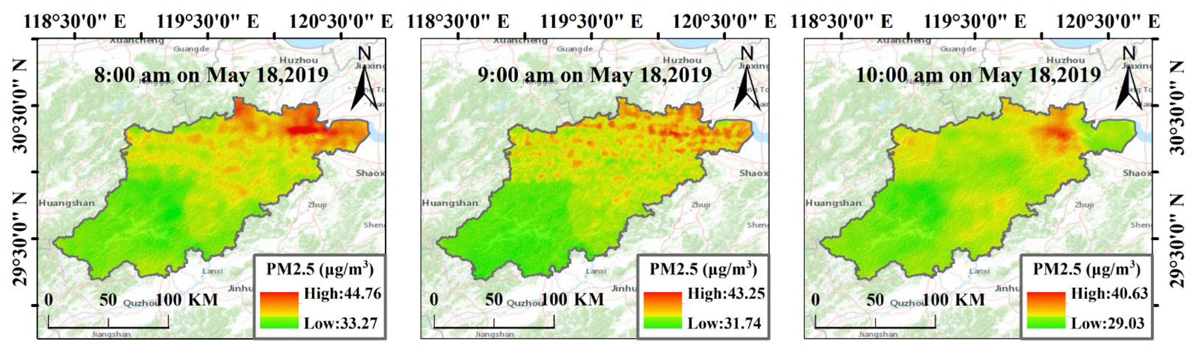
3.2. Spatiotemporal Granularity Analysis of the Retrieval Result

Here, Landsat 8 satellite images with a high spatial resolution of 30 m were used as the input variable of the retrieval model, which helps to describe the spatial details of the retrieval results. Compared with the interpolation results, these data can better reflect the spatial heterogeneity of PM2.5 distribution. Meanwhile, with the hourly meteorological data, the retrieval model realizes hourly updates of the spatial distribution of PM2.5 and can readily capture the characteristics of PM2.5 distribution. Figure 7 shows the distribution of PM2.5 at 8:00, 9:00, and 10:00 on 18 May 2019, in Hangzhou. Generally, the PM2.5 concentration in the northeast is higher than that in the southwest. However, with a change of time, the PM2.5 concentration shows a slow downward trend overall. Because around 8:00 is the peak time for work, this peak often causes the PM2.5 concentration to reach the first peak of the day, but as the traffic volume decreases, the concentration slowly decreases. At the same time, with the continuous influence of wind, the PM2.5 concentration is diluted, and the area of highly polluted regions gradually decreases. At 10:00, a highly polluted region still existed in the center of Hangzhou. This area has a high building density, a high floor, and a compact layout, which play a role in the accumulation of PM2.5 particles and are not conducive to the diffusion of particles. Therefore, the retrieval result enables a fine-grained characterization of PM2.5 in both space and time.

4. Discussion

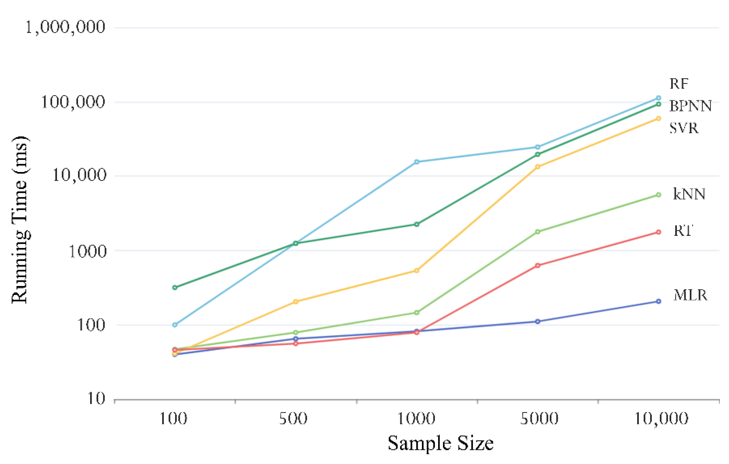
4.1. Time Efficiency of the Retrieval Model

In addition to the fitting effect, the time efficiency of the model must also be considered when performing PM2.5 remote sensing retrieval. In this paper, we used the big O notation method to express the time complexity of different algorithms and to test the time consumption of the algorithm during model training, based on different training sample sizes (100, 500, 1000, 5000, and 10,000). Here, we only focus on the difference in running time caused by the change in sample size, so each test is run based on the optimal parameters, ignoring the time consumption caused by the hyper parameters of different algorithms. The result is shown in Figure 8. Notably, the Y-axis is logarithmically scaled. This figure shows that the differences in time consumption will become more obvious with an increase of the number of samples. When the research area becomes larger or the time scale becomes longer, the time consumption of the retrieval model will increase greatly, especially when applied to the aspects that require the real-time concentration of PM2.5. Thus, time consumption will have to be considered, e.g., by using a real-time route planning with a minimum PM2.5 as the criterion [51]. Among the six algorithms, kNN achieved a relative balance between model accuracy and running time. Although the R2 (0.80) fitted by kNN was lower than the R2 (0.86) fitted by RF, when the sample size reached 10,000, the running time of kNN was only 5% of RF. With a larger sample size, this running time advantage will be more obvious. Therefore, when modeling large data volumes, decision makers must choose between time efficiency and accuracy.

4.2. Potential Room for Model Improvement

Due to the differences in PM2.5 concentration at different times, the accuracy of the retrieval model will be affected by time. In order to explore the law of model accuracy over time, the retrieval accuracy of PM2.5 concentration was evaluated at a monthly and seasonal scale. The scores of each month and season are shown in Table 5. At a monthly scale, the R2 of March and August were the highest, and the R2 of June was the lowest. At a seasonal scale, the R2 values of spring (March, April, and May) and winter (December, January, and February) were higher than those of summer (June, July, and August) and autumn (September, October, and November). Considering the significant difference of the regressing effect in different months and seasons, time series will be taken into account in future studies.
The most commonly used method to obtain the continuous PM2.5 distribution in a certain region is to interpolate the PM2.5 values measured by the air quality monitoring stations. The kriging result presented in Figure 9 was calculated via kriging interpolation of the monitored value at 11:00 on 15 April 2019, in Hangzhou, and the RF result is the distribution of PM2.5 concentration at the same time. A shortcoming of the interpolation method is that the PM2.5 concentration in the whole area is only obtained by mathematical calculations from the real measured values of the monitoring stations. Thus, the interpolation result can only represent the PM2.5 concentration distribution trend over the whole region, and the geographical unit it can represent is far less detailed than that of the retrieval model. However, at the same time, because the interpolation results are calculated from real observed values, the results can be constrained by those observed values. Thus, the closer the area is to the monitoring station, the more accurate the interpolation results will be. In contrast, the retrieval model lacks the constraints of the real values of monitoring stations, which will cause some results to deviate greatly from the real values. As illustrated in Figure 9, although the overall distribution trend of the two results is similar, there are large differences in the marked area, which indicates that the calculation errors of the retrieval model in this region are large. The same problem is also reflected in the retrieval result of RT shown in Figure 4, where a few retrieval results have large errors compared to the observed concentrations of PM2.5. We will also study the correction effects of the observed values measured by monitoring stations on the retrieval results in future research, so as to obtain more accurate PM2.5 concentration distributions.

4.3. Limitations

The method proposed in this paper has certain limitations. At present, the spatial resolution of the retrieval results in this model is affected by the spatial resolution of the Landsat satellite images. Although the spatial resolution of the Landsat 8 images is up to 30 m, this value is only a reference for the spatial resolution of the retrieval results. The current accuracy validation is based on 20140 PM2.5 observation samples from 15 air quality monitoring stations in Hangzhou from 1 April 2015, to 31 August 2019. The actual measurement data from the equipment needed to verify the accuracy of the retrieval results at a resolution of 30 m are lacking. In response to this problem, we believe that more predictors with high spatial resolutions could be added to the model in future research, such as land use cover data [52] and night light satellite data [53]. Increasing the prediction variables would help to improve the robustness of the model, greatly improving the credibility of the retrieval results.

5. Conclusions

In this study, a fine-grained PM2.5 retrieval model was proposed. This model includes high-resolution satellite image data, ground monitoring station data, and socio-economic data. We built this model based on the MLR, kNN, SVR, RT, RF, and BPNN algorithms separately and evaluated the retrieval results after a 10-fold cross-validation of each algorithm. With this model, we can retrieve the fine-grained distribution of PM2.5 every hour and dig out its change rule.
Among the six different machine learning algorithms, the RF model achieved the best retrieval effect, with the highest R2 and the highest prediction accuracy for the air quality categories. However, similar to the other five models, the RF model also showed a pattern of high prediction accuracy in low-value areas and low accuracy in high-value areas. In addition, the fitting effect of PM2.5 varied from month to month and from season to season. At a monthly level, the R2 values of March and August were the highest, at 0.84, while the R2 of June was lowest, at 0.55. At a seasonal level, the R2 values from high to low were spring, winter, autumn, and summer, reflecting the different causes of PM2.5 in different seasons. Considering that different machine learning algorithms have their own advantages, future research will take segmented regression modeling into account, in order to integrate an optimal model suitable for all regions. Future work will also focus on improving the stability of our model by expanding the research area and using more data sets.

Author Contributions

Conceptualization, P.M. and T.Z.; data curation, P.M. and L.G.; funding acquisition, F.T. and T.Z.; investigation, T.Z.; methodology, P.M. and T.Z.; project administration, F.T.; software, P.M.; supervision, T.Z.; visualization, S.L. and K.Y.; writing—original draft, L.G.; writing—review and editing, T.Z. All authors have read and agreed to the published version of the manuscript.

Funding

This research was funded by the Major project of the National Social Science Fund (19ZDA189), in part by National Natural Science Foundation of China under Grant 41301514 and Grant 41401456, in part by the Natural Science and Technology Project of Nantong (MS12020075 and MS12021082), in part by Industry-University Cooperation Collaborative Education Projects 202102245013, and in part by National College Students Innovation and Entrepreneurship Training Program (202110304041Z and 202110304108Y).

Institutional Review Board Statement

Not applicable.

Informed Consent Statement

Not applicable.

Data Availability Statement

Not applicable.

Acknowledgments

The authors would like to thank the editor and the anonymous reviewers who provided insightful comments on improving this article.

Conflicts of Interest

The authors declare no conflict of interest.

Abbreviations

The following abbreviations are used in this manuscript:
MODISModerate-resolution Imaging SpectroRadiometer
AODAerosol Optical Depth
MLRMultiple Linear Regression
SVRSupport Vector Regression
RFRandom Forest
ANNArtificial Neural Network
kNNk-nearest Neighbor
RTRegression Tree
BPNNBack Propagation Neural Network
USGSUnited States Geological Survey
FLAASHFast Line-of-sight Atmospheric Analysis of Hypercubes
CNEMCChina National Environmental Monitoring Center
CMAChina Meteorological Administration
R2Determination Coefficient
MAEMean Absolute Error
RMSERoot Mean Square Error

Appendix A

Table A1. The number of each air pollution category in the observation dataset of ground stations and the accurate number in the prediction results of the different algorithms.
CategoryObservedMLRkNNSVRRTRFBPNN
Excellent9791631280077873830889108500
Favorable8179650965856336642663726510
Light pollution16885141007794105511471205
Moderate pollution367014369144198202
Heavy pollution115016248072
Ultra-serious pollution0000000
Total20,14013,33515,75815,07415,98116,62716,489
Accuracy66%78%75%79%83%82%
Table A2. Time complexity of the algorithms and the running time under different sample sizes.
AlgorithmTime ComplexityRunning Time (ms)
1005001000500010,000
MLRO(n)406582111207
kNNO(n)477914617875602
SVRO(n2)4120553713,34059,422
RTO(nlog(n))4656796281765
RFO(nlog(n))100125115,49424,549112,265
BPNNO(n2)3171245224519,56492,817

References

  1. Lelieveld, J.; Evans, J.S.; Fnais, M.; Giannadaki, D.; Pozzer, A. The contribution of outdoor air pollution sources to premature mortality on a global scale. Nature 2015, 525, 367–371. [Google Scholar] [CrossRef] [PubMed]
  2. Han, X.; Liu, Y.; Gao, H.; Ma, J.; Mao, X.; Wang, Y.; Ma, X. Forecasting PM2.5 induced male lung cancer morbidity in China using satellite retrieved PM2.5 and spatial analysis. Sci. Total Environ. 2017, 607–608, 1009–1017. [Google Scholar] [CrossRef] [PubMed]
  3. Turner, M.C.; Krewski, D.; Pope, C.A.; Chen, Y.; Gapstur, S.M.; Thun, M.J. Long-term ambient fine particulate matter air pollution and lung cancer in a large cohort of never-smokers. Am. J. Respir. Crit. Care Med. 2011, 184, 1374–1381. [Google Scholar] [CrossRef] [PubMed]
  4. Yang, Q.; Yuan, Q.; Li, T.; Yue, L. Mapping PM2.5 concentration at high resolution using a cascade random forest based downscaling model: Evaluation and application. J. Clean. Prod. 2020, 277, 123887. [Google Scholar] [CrossRef]
  5. Meng, X.; Liu, C.; Zhang, L.; Wang, W.; Stowell, J.; Kan, H.; Liu, Y. Estimating PM2.5 concentrations in Northeastern China with full spatiotemporal coverage, 2005–2016. Remote Sens. Environ. 2021, 253, 112203. [Google Scholar] [CrossRef]
  6. Chen, W.; Ran, H.; Cao, X.; Wang, J.; Teng, D.; Chen, J.; Zheng, X. Estimating PM2.5 with high-resolution 1-km AOD data and an improved machine learning model over Shenzhen, China. Sci. Total Environ. 2020, 746, 141093. [Google Scholar] [CrossRef]
  7. Pak, U.; Ma, J.; Ryu, U.; Ryom, K.; Juhyok, U.; Pak, K.; Pak, C. Deep learning-based PM2.5 prediction considering the spatiotemporal correlations: A case study of Beijing, China. Sci. Total Environ. 2020, 699, 133561. [Google Scholar] [CrossRef]
  8. Li, L. A robust deep learning approach for spatiotemporal estimation of Satellite AOD and PM2.5. Remote Sens. 2020, 12, 264. [Google Scholar] [CrossRef] [Green Version]
  9. van Donkelaar, A.; Martin, R.V.; Brauer, M.; Kahn, R.; Levy, R.; Verduzco, C.; Villeneuve, P.J. Global estimates of ambient fine particulate matter concentrations from satellite-based aerosol optical depth: Development and application. Environ. Health Perspect. 2010, 118, 847–855. [Google Scholar] [CrossRef] [Green Version]
  10. Chen, X.; Li, H.; Zhang, S.; Chen, Y.; Fan, Q. High Spatial Resolution PM2.5 Retrieval Using MODIS and Ground Observation Station Data Based on Ensemble Random Forest. IEEE Access 2019, 7, 44416–44430. [Google Scholar] [CrossRef]
  11. Yazdi, M.D.; Kuang, Z.; Dimakopoulou, K.; Barratt, B.; Suel, E.; Amini, H.; Lyapustin, A.; Katsouyanni, K.; Schwartz, J. Predicting fine particulate matter (PM2.5) in the greater london area: An ensemble approach using machine learning methods. Remote Sens. 2020, 12, 914. [Google Scholar] [CrossRef] [Green Version]
  12. Ma, Z.; Hu, X.; Huang, L.; Bi, J.; Liu, Y. Estimating ground-level PM2.5 in china using satellite remote sensing. Environ. Sci. Technol. 2014, 48, 7436–7444. [Google Scholar] [CrossRef] [PubMed]
  13. Zou, B.; Zheng, Z.; Wan, N.; Qiu, Y.; Wilson, J.G. An optimized spatial proximity model for fine particulate matter air pollution exposure assessment in areas of sparse monitoring. Int. J. Geogr. Inf. Sci. 2016, 30, 727–747. [Google Scholar] [CrossRef]
  14. de Hoogh, K.; Héritier, H.; Stafoggia, M.; Künzli, N.; Kloog, I. Modelling daily PM2.5 concentrations at high spatio-temporal resolution across Switzerland. Environ. Pollut. 2018, 233, 1147–1154. [Google Scholar] [CrossRef]
  15. Unnithan, S.L.K.; Gnanappazham, L. Spatiotemporal mixed effects modeling for the estimation of PM2.5 from MODIS AOD over the Indian subcontinent. GISci. Remote Sens. 2020, 57, 159–173. [Google Scholar] [CrossRef]
  16. Liu, Y.; Park, R.J.; Jacob, D.J.; Li, Q.; Kilaru, V.; Sarnat, J.A. Mapping annual mean ground-level PM2.5 concentrations using Multiangle Imaging Spectroradiometer aerosol optical thickness over the contiguous United States. J. Geophys. Res. D Atmos. 2004, 109, 3269–3278. [Google Scholar]
  17. Liu, Y.; Sarnat, J.A.; Kilaru, V.; Jacob, D.J.; Koutrakis, P. Estimating ground-level PM2.5 in the eastern United States using satellite remote sensing. Environ. Sci. Technol. 2005, 39, 3269–3278. [Google Scholar] [CrossRef] [Green Version]
  18. Zeng, Q.; Tao, J.; Chen, L.; Zhu, H.; Zhu, S.Y.; Wang, Y. Estimating ground-level particulate matter in five regions of China using aerosol optical depth. Remote Sens. 2020, 12, 881. [Google Scholar] [CrossRef] [Green Version]
  19. Lee, H.J.; Liu, Y.; Coull, B.A.; Schwartz, J.; Koutrakis, P. A novel calibration approach of MODIS AOD data to predict PM2.5 concentrations. Atmos. Chem. Phys. 2011, 11, 7991–8002. [Google Scholar] [CrossRef] [Green Version]
  20. Zhang, T.; Zhu, Z.; Gong, W.; Zhu, Z.; Sun, K.; Wang, L.; Huang, Y.; Mao, F.; Shen, H.; Li, Z.; et al. Estimation of ultrahigh resolution PM2.5 concentrations in urban areas using 160 m Gaofen-1 AOD retrievals. Remote Sens. Environ. 2018, 216, 91–104. [Google Scholar] [CrossRef]
  21. Sun, L.; Wei, J.; Bilal, M.; Tian, X.; Jia, C.; Guo, Y.; Mi, X. Aerosol optical depth retrieval over bright areas using Landsat 8 OLI images. Remote Sens. 2016, 8, 23. [Google Scholar] [CrossRef] [Green Version]
  22. Xu, J.; Han, F.; Li, M.; Zhang, Z.; Xiaohui, D.; Wei, P. On the opposite seasonality of MODIS AOD and surface PM2.5 over the Northern China plain. Atmos. Environ. 2019, 215, 116909. [Google Scholar] [CrossRef]
  23. Yang, Q.; Yuan, Q.; Yue, L.; Li, T.; Shen, H.; Zhang, L. The relationships between PM2.5 and aerosol optical depth (AOD) in mainland China: About and behind the spatio-temporal variations. Environ. Pollut. 2019, 248, 526–535. [Google Scholar] [CrossRef] [PubMed]
  24. Zhang, B.; Zhang, M.; Kang, J.; Hong, D.; Xu, J.; Zhu, X. Estimation of PMx Concentrations from Landsat 8 OLI Images Based on a Multilayer Perceptron Neural Network. Remote Sens. 2019, 11, 646. [Google Scholar] [CrossRef] [Green Version]
  25. Yun, G.; Zuo, S.; Dai, S.; Song, X.; Id, C.X.; Liao, Y.; Zhao, P.; Chang, W.; Id, Q.C.; Li, Y.; et al. Individual and Interactive Influences of Anthropogenic and Ecological Factors on Forest PM2.5 Concentrations at an Urban Scale. Remote Sens. 2018, 10, 521. [Google Scholar] [CrossRef] [Green Version]
  26. Liu, J.; Weng, F.; Li, Z.; Cribb, M.C. Hourly PM2.5 estimates from a geostationary satellite based on an ensemble learning algorithm and their spatiotemporal patterns over central East China. Remote Sens. 2019, 11, 2120. [Google Scholar] [CrossRef] [Green Version]
  27. He, Q.; Huang, B. Satellite-based high-resolution PM2.5 estimation over the Beijing-Tianjin-Hebei region of China using an improved geographically and temporally weighted regression model. Environ. Pollut. 2018, 236, 1027–1037. [Google Scholar] [CrossRef]
  28. Kaimian, H.; Li, Q.; Wu, C.; Qi, Y.; Mo, Y.; Chen, G.; Zhang, X.; Sachdeva, S. Evaluation of different machine learning approaches to forecasting PM2.5 mass concentrations. Aerosol. Air Qual. Res. 2019, 19, 1400–1410. [Google Scholar] [CrossRef] [Green Version]
  29. Stadlober, E.; Hörmann, S.; Pfeiler, B. Quality and performance of a PM10 daily forecasting model. Atmos. Environ. 2008, 42, 1098–1109. [Google Scholar] [CrossRef]
  30. Drucker, H.; Burges, C.J.C.; Kaufman, L.; Smola, A.; Vapoik, V.; Long, W.; Nj, B. Support Vector Regression Machines. Neural Inf. Process. 1996, 28, 779–784. [Google Scholar]
  31. Zhu, S.; Lian, X.; Wei, L.; Che, J.; Shen, X.; Yang, L.; Qiu, X.; Liu, X.; Gao, W.; Ren, X.; et al. PM2.5 forecasting using SVR with PSOGSA algorithm based on CEEMD, GRNN and GCA considering meteorological factors. Atmos. Environ. 2018, 183, 20–32. [Google Scholar] [CrossRef]
  32. Voukantsis, D.; Karatzas, K.; Kukkonen, J.; Räsänen, T.; Karppinen, A.; Kolehmainen, M. Intercomparison of air quality data using principal component analysis, and forecasting of PM10 and PM2.5 concentrations using artificial neural networks, in Thessaloniki and Helsinki. Sci. Total Environ. 2011, 409, 1266–1276. [Google Scholar] [CrossRef] [PubMed]
  33. Li, L.; Chen, B.; Zhang, Y.; Zhao, Y.; Xian, Y.; Xu, G.; Zhang, H.; Guo, L. Retrieval of daily PM2.5 concentrations using nonlinear methods: A case study of the Beijing-Tianjin-Hebei Region, China. Remote Sens. 2018, 10, 2006. [Google Scholar] [CrossRef] [Green Version]
  34. Bai, Y.; Wu, L.; Qin, K.; Zhang, Y.; Shen, Y.; Zhou, Y. A geographically and temporally weighted regression model for ground-level PM2.5 estimation from satellite-derived 500 m resolution AOD. Remote Sens. 2016, 8, 262. [Google Scholar] [CrossRef] [Green Version]
  35. Yang, H.; Chen, W.; Liang, Z. Impact of land use on PM2.5 pollution in a representative city of middle China. Int. J. Environ. Res. Public Health 2017, 14, 462. [Google Scholar] [CrossRef]
  36. Askariyeh, M.H.; Zietsman, J.; Autenrieth, R. Traffic contribution to PM2.5 increment in the near-road environment. Atmos. Environ. 2020, 224, 117113. [Google Scholar] [CrossRef]
  37. Han, D.; Gao, S.; Fu, Q.; Cheng, J.; Chen, X.; Xu, H.; Liang, S.; Zhou, Y.; Ma, Y. Do volatile organic compounds (VOCs) emitted from petrochemical industries affect regional PM2.5? Atmos. Res. 2018, 209, 123–130. [Google Scholar] [CrossRef]
  38. Cooley, T.; Anderson, G.P.; Felde, G.W.; Hoke, M.L.; Ratkowski, A.J.; Chetwynd, J.H.; Gardner, J.A.; Adler-Golden, S.M.; Matthew, M.W.; Berk, A.; et al. FLAASH, a MODTRAN4-based atmospheric correction algorithm, its applications and validation. Int. Geosci. Remote Sens. Symp. 2002, 3, 1414–1418. [Google Scholar]
  39. Tobler, W.R. A Computer Movie Simulating Urban Growth in the Detroit Region. Econ. Geogr. 1970, 46, 234–240. [Google Scholar] [CrossRef]
  40. Pal, M.; Bharati, P. Introduction to correlation and linear regression analysis. In Applications of Regression Techniques; Springer: Berlin/Heidelberg, Germany, 2019; pp. 1–18. [Google Scholar]
  41. Qian, Y.; Zhou, W.; Yan, J.; Li, W.; Han, L. Comparing machine learning classifiers for object-based land cover classification using very high resolution imagery. Remote Sens. 2015, 7, 153–168. [Google Scholar] [CrossRef]
  42. Tao, Y.; Yan, H.; Gao, H.; Sun, Y.; Li, G. Application of SVR optimized by modified simulated annealing (MSA-SVR) air conditioning load prediction model. J. Ind. Inf. Integr. 2019, 15, 247–251. [Google Scholar] [CrossRef]
  43. Lu, H.; Ma, X. Hybrid decision tree-based machine learning models for short-term water quality prediction. Chemosphere 2020, 249, 126169. [Google Scholar] [CrossRef] [PubMed]
  44. Wang, W.; Zhao, S.; Jiao, L.; Taylor, M.; Zhang, B.; Xu, G.; Hou, H. Estimation of PM2.5 concentrations in China using a spatial back propagation neural network. Sci. Rep. 2019, 9, 13788. [Google Scholar] [CrossRef] [PubMed] [Green Version]
  45. Cawley, G.C.; Talbot, N.L.C. On over-fitting in model selection and subsequent selection bias in performance evaluation. J. Mach. Learn. Res. 2010, 11, 2079–2107. [Google Scholar]
  46. Zhang, H.; Kondragunta, S. Daily and Hourly Surface PM2.5 Estimation From Satellite AOD. Earth Space Sci. 2021, 8, e2020EA001599. [Google Scholar] [CrossRef]
  47. Xue, W.; Zhang, J.; Zhong, C.; Li, X.; Wei, J. Spatiotemporal PM2.5 variations and its response to the industrial structure from 2000 to 2018 in the Beijing-Tianjin-Hebei region. J. Clean. Prod. 2021, 279, 123742. [Google Scholar] [CrossRef]
  48. Chen, Z.; Hao, X.; Zhang, X.; Chen, F. Have traffic restrictions improved air quality? A shock from COVID-19. J. Clean. Prod. 2021, 279, 123622. [Google Scholar] [CrossRef]
  49. Yuan, M.; Huang, Y.; Shen, H.; Li, T. Effects of urban form on haze pollution in China: Spatial regression analysis based on PM2.5 remote sensing data. Appl. Geogr. 2018, 98, 215–223. [Google Scholar] [CrossRef]
  50. Li, X.; Wu, C.; Meadows, M.E.; Zhang, Z.; Lin, X.; Zhang, Z.; Chi, Y.; Feng, M.; Li, E.; Hu, Y. Factors underlying spatiotemporal variations in atmospheric pm2.5 concentrations in zhejiang province, china. Remote Sens. 2021, 13, 3011. [Google Scholar] [CrossRef]
  51. Gao, L.-N.; Tao, F.; Ma, P.-L.; Wang, C.-Y.; Kong, W.; Chen, W.-K.; Zhou, T. A short-distance healthy route planning approach. J. Transp. Health 2022, 24, 101314. [Google Scholar] [CrossRef]
  52. Reid, C.E.; Jerrett, M.; Petersen, M.L.; Pfister, G.G.; Morefield, P.E.; Tager, I.B.; Raffuse, S.M.; Balmes, J.R. Spatiotemporal prediction of fine particulate matter during the 2008 Northern California wildfires using machine learning. Environ. Sci. Technol. 2015, 49, 3887–3896. [Google Scholar] [CrossRef] [PubMed]
  53. Wang, Y.; Wang, M.; Huang, B.; Li, S.; Lin, Y. Estimation and analysis of the nighttime PM2.5 concentration based on lj1-01 images: A case study in the pearl river delta urban agglomeration of china. Remote Sens. 2021, 13, 3405. [Google Scholar] [CrossRef]
Figure 1. Location map and topographic map of the study area.
Remotesensing 14 00599 g001
Figure 2. Methodological framework of the study.
Remotesensing 14 00599 g002
Figure 3. Schematic diagram of 10-fold cross-validation. E represents the total error of the model. Ei (i = 1, 2, 3 …… 10) represents the error at the   i th iteration, and E is calculated by averaging the sum of Ei.
Remotesensing 14 00599 g003
Figure 4. PM2.5 concentration at 11:00 on 15 April 2019, based on the retrieval model built by different machine learning algorithms.
Remotesensing 14 00599 g004
Figure 5. Scatter plots of the observed and predicted values of the different algorithms: (a) MLR, (b) kNN, (c) SVR, (d) RT, (e) RF, (f) BPNN. The Y-axis is the PM2.5 value observed by 15 air quality monitoring stations in Hangzhou from 1 April 2015, to 31 August 2019, the X-axis is the PM2.5 value predicted by the retrieval model, and the number of sample points is 20140.
Remotesensing 14 00599 g005
Figure 6. Performance of different machine learning algorithms in predicting the PM2.5 pollution categories: (a) MLR, (b) kNN, (c) SVR, (d) RT, (e) RF, (f) BPNN. Each subplot presents a comparison of the predicted results of an algorithm with the observed results. The closer the predicted result was to the observed result, the stronger the algorithm’s ability to predict the pollution categories. The X-axis represents the different pollution categories, the main Y-axis represents the number of each category, and the secondary Y-axis represents the prediction accuracy for each category. The detailed data used for developing this figure are shown in Table A1.
Remotesensing 14 00599 g006
Figure 7. PM2.5 retrieval results at 8:00, 9:00, and 10:00 on 18 May 2019.
Remotesensing 14 00599 g007
Figure 8. Running times of the different algorithms under different sample sizes. As the running time span is large, a logarithmic scale (logBase = 10) is used here for the Y-axis to balance the image content. The specific running time and corresponding time complexity are shown in Table A2.
Remotesensing 14 00599 g008
Figure 9. PM2.5 distribution results of kriging interpolation and RF model.
Remotesensing 14 00599 g009
Table 1. The list of datasets with their sources and download links.
CategorySourceAccessed DateUniform Resource Location
Landsat imagesUSGS15 January 2020https://earthexplorer.usgs.gov/
PM2.5CNEMC15 January 2020http://www.cnemc.cn/
MeteorologicalCMA15 January 2020http://www.cma.gov.cn/
GDP RESDC2 March 2020http://www.resdc.cn/
POPRESDC2 March 2020http://www.resdc.cn/
Industry BaiduMap5 March 2020https://lbsyun.baidu.com/
Road NetworksOpenStreetMap5 March 2020https://www.openstreetmap.org/
Table 2. Eigenvalues of different models. The number in the double brackets represents the difference between the predicted value and the observed value. The ‘+’ sign means larger than the observed value, and the ‘−’ sign means smaller than the observed value. Bold numbers indicate the closest result to the observed value.
ModelMin (μg/m3)Max (μg/m3)Mean (μg/m3)Median (μg/m3)
Observed1.0198.0842.3035.77
MLR−57.73 (−58.73)121.56 (−76.52)42.30 (0)39.96 (+4.19)
KNN3.92 (+2.92)162.91 (−35.17)42.34 (+0.04)36.47 (+0.70)
SVR1.36 (+0.36)152.31 (−45.77)41.00 (−1.30)36.32 (+0.55)
RT1.0 (0)195.88 (−2.20)42.49 (+0.19)36.36 (+0.59)
RF5.74 (+4.74)154.19 (−43.89)42.42 (+0.12)37.00 (+1.23)
BPNN7.34 (+6.34)182.94 (15.14)41.51 (−0.79)34.45 (−1.32)
Table 3. Validation index score.
ModelMAE (μg/m3)RMSE (μg/m3)R2
MLR13.2918.780.51
kNN8.2811.800.80
SVR10.1115.050.68
RT8.2412.600.78
RF6.7210.110.86
BPNN7.1410.370.85
Table 4. Comparison of variable importance and correlation ranking. xDB refers to the average PM2.5 concentration x day(s) before. The ‘↑’ sign indicates that the ranking of variable importance has increased compared to the rank of the correlation, the ‘↓’ sign indicates that the ranking of variable importance has decreased compared to the rank of the correlation, and the ‘-’ sign indicates that the ranking did not change.
VariableImportance RankingCorrelation RankingRanking Change
1DB11-
PREC210↑ 8
WS39↑ 6
TEMP43↓ 1
2DB52↓ 3
RH618↑ 12
6DB77-
7DB85↓ 3
4DB96↓ 3
3DB104↓ 6
POP1113↑ 2
Industry1214↑ 2
Road1312↓ 1
GDP1416↑ 2
Band 51511↓ 4
NDVI1623↑ 7
Band 71722↑ 5
Band 61815↓ 3
Band 41921↑ 2
Band 32017↓ 3
Band 12120↓ 1
Band 22219↓ 3
Table 5. Scores of the different months and seasons. The data used in this experiment were obtained from 1 April 2015 to 31 August 2019.
TimeMAE (μg/m3)RMSE (μg/m3)R2
January10.0813.850.85
February8.8012.870.83
March7.6810.970.84
April5.307.430.77
May5.928.840.81
June7.4213.020.55
July4.496.650.75
August4.436.030.84
September4.666.800.77
October7.3410.780.81
November6.809.000.71
December9.8613.960.82
Spring6.8410.040.82
Summer5.208.390.71
Autumn6.169.090.78
Winter10.0914.540.80
Publisher’s Note: MDPI stays neutral with regard to jurisdictional claims in published maps and institutional affiliations.

