A Simple Cloud-Native Spectral Transformation Method to Disentangle Optically Shallow and Deep Waters in Sentinel-2 Images

Abstract

This study presents a novel method to identify optically deep water using purely spectral approaches. Optically deep waters, where the seabed is too deep for a bottom reflectance signal to be returned, is uninformative for seabed mapping. Furthermore, owing to the attenuation of light in the water column, submerged vegetation at deeper depths is easily confused with optically deep waters, thereby inducing misclassifications that reduce the accuracy of these seabed maps. While bathymetry data could mask out deeper areas, they are not always available or of sufficient spatial resolution for use. Without bathymetry data and based on the coastal aerosol blue green (1-2-3) bands of the Sentinel-2 imagery, this study investigates the use of band ratios and a false colour HSV transformation of both L1C and L2A images to separate optically deep and shallow waters across varying water quality over four tropical and temperate submerged sites: Tanzania, the Bahamas, the Caspian Sea (Kazakhstan) and the Wadden Sea (Denmark and Germany). Two supervised thresholds based on annotated reference data and an unsupervised Otsu threshold were applied. The band ratio group usually featured the best overall accuracies (OA), F1 scores and Matthews correlation coefficients, although the individual band combination might not perform consistently across different sites. Meanwhile, the saturation and hue band yielded close to best performance for the L1C and L2A images, featuring OA of up to 0.93 and 0.98, respectively, and a more consistent behaviour than the individual band ratios. Nonetheless, all these spectral methods are still susceptible to sunglint, the Sentinel-2 parallax effect, turbidity and water colour. Both supervised approaches performed similarly and were superior to the unsupervised Otsu’s method—the supervised methods featuring OA were usually over 0.70, while the unsupervised OA were usually under 0.80. In the absence of bathymetry data, this method could effectively remove optically deep water pixels in Sentinel-2 imagery and reduce the issue of dark pixel misclassification, thereby improving the benthic mapping of optically shallow waters and their seascapes.

1. Introduction

Coastal seascape ecosystems such as seagrasses and coral reefs provide a multitude of highly valued services such as coastal protection, biodiversity maintenance, blue carbon sequestration as well as nursery and feeding grounds for many marine animals [1]. However, these ecosystems are also highly threatened and thus require urgent conservation and monitoring efforts [1,2]. Coastal aquatic remote sensing can help monitor these ecosystems by providing information on their benthic composition, water quality and bathymetry. Unlike terrestrial remote sensing, aquatic applications require an additional consideration of the water column and its interactions with the light signal [3], which has implications for seabed signals.

1.1. Seabed Remote Sensing

When the object(s) of interest is located on the benthic floor and not floating near the water surface, the depth affects the attenuation of the water column and its constituents [4,5] on the return signals [6], which modifies the spectral profile of the reflected signal with increasing depth [7]. This effect on the benthic spectral signature not only reduces the spectral difference between benthic classes [7,8,9] but also restricts the informative bands mostly to the visible spectrum [4,10,11]. With sufficient depth, all information on the benthic cover is lost, and only the backscattering of the water column remains in these so-called optically deep waters [4,5]. These non-informative pixels should be removed from a seabed image, especially since some classes such as the darker seagrasses are easily confused with these deep waters [4,9,12]. However, identifying these optically deep waters can be a challenge.

There are many approaches to manage this, such as through water column correction, using bathymetry data or satellite-derived bathymetry (SDB) [13,14,15], object-based image analysis [7] and machine learning techniques [16]. Bathymetric data are usually exploited, since pixels deeper than 10 m have very weak benthic signals [5] or are quasi-optically deep [4]. Nonetheless, the benthic floor is still detectable in optimal conditions up to about 43 m [17]. The optical limit is also highly influenced by water quality, bottom cover and optical conditions during image acquisition [4], thereby suggesting potential information loss with an arbitrary depth threshold. Alternatively, semi-analytical approaches [4,15,18] such as the substratum detectability index (SDI) [5] could identify the optically shallow, quasi-optically deep and optically deep pixels via radiative transfer models. However, these underlying models are highly technical and might put off non-specialist researchers. Naturally, manual digitisation via photointerpretation is possible but labour-intensive [19]. Thus, it would still be optimal to have a simple yet effective method for masking out optically deep waters.

Such an approach might be possible when there is a correlation between pixel values and depth [20], such as band ratios [20,21,22] or logarithmic-transformed band ratio [18,23,24]. While deriving bathymetry would require external data for depth calibration, Legleiter et al. [20] found a strong linear relationship between radiometric values and bathymetry depth in shallow river waters up to 1 m in depth, which could be extended to identify optically deep water pixels without bathymetric information. Nonetheless, the choice of band ratio is important, as shorter wavelengths have greater depth penetration but are susceptible to turbidity, while longer wavelengths, such as the red band with its limit of about 5 m [25], do not provide sufficient penetration or range [8,17]. Existing optimisation approaches for depth estimation such as the Optimised Band Ratio Analysis (OBRA), Multiple Optimal Depth Predictors Analysis (MODPA) and the Sample-specific Multiple Band Ratio Techniques for SDB (SMART-SDB) [20,26,27] can naturally be translated to the detection of the optically deep and shallow waters. Nonetheless, given the challenges of the band ratios as well as the limited number of informative bands, alternative spectral approaches might prove helpful.

1.2. Colour Spaces in Remote Sensing

Multispectral and hyperspectral remote sensing both lie in the red-green-blue (RGB) colour space, expanding from three primary hues or wavelengths to the number of bands detected [4]. While the RGB system is based on the physics of light, sometimes an RGB image may not look similar to its supposed colour given its wavelength inputs [28,29]. Alternatively, the hue-saturation-luminosity colour space is based on the colour perception of a normal human [28]. By considering the full colour spectrum as a wheel with red as the origin, the hue or a human-perceived colour is the angle on this colour wheel, while saturation is the richness of a colour with respect to its luminosity or brightness. Both hue and saturation describe the spectral shape of a signal [28]. While there might be different luminosity variables, the “value” is used for the hue-saturation-value (HSV) colour space.

The use of the HSV colour space is not new to remote sensing. Some of its applications include cloud and cloud shadow detection [30,31], crop and farmland detection [32,33], algal bloom detection [34], surface water extraction and river extraction [35,36], oceanic water assessments [37] and water quality retrieval [29,38]. Most recently, Lee et al. [6] related the true colour hue angle to the vertical variation of light quality in marine waters, as well as the different optical water types, which represent different aquatic environments globally [39,40]. Many applications rely on a true colour RGB to HSV transformation, even when using a hyperspectral sensor [41]. However, the red wavelength, with its low penetrative property, is less useful at deeper depths [8]. An alternative is to transform a false colour RGB image instead, as there are no restrictions on the input bands [41]. The false colour RGB is most notably seen in band combinations for visualisation purposes and has been used to successfully detect global surface water using the high-resolution Landsat series [42]. In conjunction with the aforementioned difference in depth penetration between wavelengths as well as the general use of blue and green bands for oceanic remote sensing [43], this theoretically suggests that a coastal aerosol-blue-green wavelength (~430–560 nm central wavelength range) false-colour-derived HSV image could provide the required information to distinguish between the optically deep and shallow water pixels.

1.3. Study Aim

We employ Sentinel-2 imagery to develop and test our method as it features the aforementioned wavelengths of interest, high spatial resolution of 10 m, high temporal resolution of 5 days and widespread use in coastal aquatic remote sensing. By focusing on the bands B1–B3, this study aims to investigate if the resultant band ratios and coastal aerosol-blue-green false colour HSV transformation of the Sentinel-2 L1C and L2A images can distinguish between optically deep and optically shallow waters in the absence of bathymetry data.

2. Materials and Methods

2.1. Study Area and Data

Four sites were selected based on different environmental conditions in order to investigate the effectiveness of the different indices in these conditions (

Table 1. Test site descriptions.

Site, Country	Site Description	Satellite Image Id
Unguja, Tanzania	Single scene, coastal/marine, tropical, sunglinted	20191207T073209_20191207T074734_T37MEP
Andros and Nassau, The Bahamas	Single scene, coastal/marine, tropical	20191119T155531_20191119T155526_T17RRH
Caspian Sea, Kazakhstan	Single scene, freshwater, temperate, turbid	20190610T072629_20190610T073416_T39TVK
Wadden Sea, Germany and Denmark	Single scene, coastal/marine, temperate, turbid	20190617T104029_20190617T104030_T32UMF

and Figure 1). The images were either cloud-free or contained as little cloud cover as possible. The Tanzanian and Bahamian sites were chosen as representatives of tropical, coastal waters. While the selected image of the former had issues with sunglint, the selected Bahamian image had highly optimal conditions. Meanwhile, the Caspian Sea and Wadden Sea feature highly turbid, temperate waters of inland freshwater and coastal marine waters, respectively.

The following datasets were used: Sentinel-2 MSI: MultiSpectral Instrument, Top-Of-Atmosphere Level-1C (L1C) and Sentinel-2 MSI: MultiSpectral Instrument, Bottom-Of-Atmosphere Level-2A (L2A).

2.2. Preprocessing

Most of the processing was performed in the Google Earth Engine (GEE) cloud computing platform [44]. Thus, unless otherwise stated, any functions mentioned are GEE native functions, products or datasets. The same image ID was used for both the L1C and L2A products (Table 1). Clouds were excluded using both the QA band and the Sentinel-2: Cloud Probability dataset set to 40% threshold. Although the atmospheric correction for air and water column is the standard for coastal water image analysis [9], Lee et al. [16] was able to bypass atmospheric correction by using machine learning methods for their semi-analytical model on Landsat 8 TOA images while Thomas et al. [45] deliberately did not perform any atmospheric correction in order to evaluate the errors between using Sentinel-2 L1C and L2A products for their SDB method. As the preliminary trials had shown that no further atmospheric corrections were required when applying this method onto single scenes, the corrections were not performed. In line with Thomas et al. [45], sunglint correction was also not performed in order to investigate its effects on the methods of interest.

An adaptive Otsu’s threshold of the NDWI was then applied to all images of both products to mask out the land pixels [46].

2.3. Vector Dataset and Indices

Fifty line vectors were manually digitised from their corresponding scenes by visual interpretation on the GEE web-based interface. Since the optically deep property is similar to an apparent optical property, it is an image-specific property related to bathymetric depth but is scene and sensor dependent [5]. Unlike the SDI [5], only two classes of optically deep and shallow were selected, for the quasi-optically deep class was ignored due to the difficulty in visually distinguishing it from the two other classes. The deep water regions were determined by a consistent, large area of dark pixels that is connected to the larger ocean or sea in the image and thus could be distinguished from deeper but still optically shallow dark benthic cover. From the visually identified shallow-deep boundary, line vectors were drawn on both sides of the boundary which are perpendicular to the shore to imitate a field survey’s line transect from shallow to deep and to better represent this gradual gradient between classes. Each transect consists of one deep water and one shallow water vector of similar length. In areas where a clear and distinct shallow-deep boundary could not be identified, no vectors were drawn. For areas in which the optically shallow-deep border is insufficient to contain all the vectors without possible spatial autocorrelation, the remaining vectors were annotated on suitable pixels in the image (Figure 2).

As the line vectors are created via photointerpretation, there would naturally be some biases in the base image. As such, bathymetric inputs from ETOPO1 Global Arc-Minute Elevation (ETOPO) [47], General Bathymetric Chart of the Oceans (GEBCO) [48] and a Sentinel-2 image-based SDB [15] were used to evaluate the labels for all sites. As the ICESAT-2 data for 2018 and 2021 are available for the Bahamian site, an SDB was created from the same image in Table 1 based on a 7:3 split using three approaches—spatial, random and temporal [45]. In addition, K_d photosynthetically active radiation (PAR) and seabed PAR dataset for 2005–2009 by the European Marine Observation and Data Network (EMODnet) are available at the Wadden Sea site to assess light penetration into the water column [49]. Other than the image-based SDB method, these auxiliary datasets were not of the same time period as the images, as the images were pre-selected, as described in Section 2.1. A comparison of depth values between classes using the Welch’s unequal variance t-test was performed in R version 4.1.0 [50]. The choice of a continuous instead of a binary optically deep-optically shallow comparison was because the binary requires a photointerpretation of the depth to the class labels in the image (s). That would have defeated the purpose of this calibration. However, the combined analysis from all these datasets showed that the vectors were reasonably placed to detect and label pixels as optically deep and optically shallow (Figure 3) given their very significantly different group means (all p values < 0.001). Nonetheless, a single depth threshold is insufficient as a blanket cut-off across a single image, as seen by some overlaps in bathymetry depth values between the optically deep and optically shallow vectors. This is especially valid for the coarser resolution of the ETOPO1, GEBCO and EMODnet dataset. Nonetheless, most sites do not have an overlap in the interquartile ranges except for Tanzania (Figure 3), these line vectors are deemed sufficient for use in this study. The reader is directed to Appendix A

Table A1. Welch’s test p-value in scientific form showing difference in group means between optically deep and optically shallow classes over four single scene Sentinel-2 images. The results for the L1C and L2A products are highly similar. The greyed cells indicate an absence of valid data for the site. ETOPO—ETOPO1 Global Arc-Minute Elevation, GEBCO—the General Bathymetric Chart of the Oceans, SDB—Sentinel-2 image-based satellite derived bathymetry based on [18], the I-S—ICESAT2 derived SDB based on [51] using a pooled ICESAT2 data that was spatially split, I-S ICESAT2 which data was randomly split, I-S—ICESAT2 which data was temporally split (ICESAT-T), E-K—the European Marine Observation and Data Network dataset for K_d PAR (EMODnet-K), E-S—the EMODnet dataset for seabed PAR (EMODnet-S).

Site	ETOPO	GEBCO	SDB	I-S	I-R	I-T	E-K	E-S
Bahamas	2.8 × 10−13	2.2 × 10−16	2.2 × 10−16	2.2 × 10−16	2.2 × 10−16	2.2 × 10−16
Caspian Sea	3.1 × 10−6	2.2 × 10−16	2.2 × 10−16
Tanzania	2.7 × 10−4	1.1 × 10−11	2.2 × 10−16
Wadden Sea	2.2 × 10−16	2.2 × 10−16	2.2 × 10−16				2.2 × 10−16	2.2 × 10−16

for the p values of all test combinations.

A 7:3 training–validation data (training data—TD, validation data—VD) split of the vector dataset was performed for the subsequent k-fold cross-validation, where k = 10 as commonly used in literature [51] and based on the GEE seeds 0 to 9 in the randomColumn function. The same images were used as the optically deep–shallow boundary was observed to have marginal temporal shifts owing to slightly temporally different environments. Subsequently, this small border shift might affect the ends of drawn transects and contribute to the mislabelling of border pixels, which are crucial for determining the threshold between the two optical classes.

Six indices were compared in this study—the three 1-2-3 false colour HSV bands and the band ratios B1/B2, B1/B3 and B2/B3 (Figure 4 and Figure 5). B1, B2 and B3 were selected as they have the best penetration, which means that they are more likely to pick up the bottom signal at deeper depths than the other bands, such as B4, which attenuates fast [8,52]. A 3 × 3 low pass filter was used to smoothen the image before the transformations.

For the HSV bands, the rgbToHsv function was used to transform the 1-2-3 false colour image to obtain its HSV components as seen in Figure 4 and Figure 5. This function in GEE is based on Java’s Color: RGBtoHSB function, which is normalised to a scale between 0 and 1 as well as based on standard HSV transformation algorithms [28,29]:

$$∆=Cmax-Cmin$$

(1)

$$Saturation=\{\begin{array}{cc}0& ,Cmax=0\\ \frac{∆}{Cmax}& ,Cmax\ne 0\end{array}$$

(2)

$$Hue=\{\begin{array}{ccc}0& ,& ∆=0\\ \frac{1}{6}\times \left(\frac{G-B}{∆}\right)& ,& Cmax=R,G>B\\ 1-\frac{1}{6}\times \left(\frac{G-B}{∆}\right)& ,& Cmax=R,G<B\\ \frac{1}{3}+\frac{1}{6}\times \left(\frac{B-R}{∆}\right)& ,& Cmax=G\\ \frac{2}{3}+\frac{1}{6}\times \left(\frac{R-G}{∆}\right)& ,& Cmax=B\end{array}$$

(3)

$$Value=\{\begin{array}{cc}Cmax& ,Cmax<1\\ 1& ,Cmax\ge 1\end{array}$$

(4)

The band ratios are an extension of Lyzenga’s relative depth index [18,23,24]. While many studies employed log-transformed band ratios [20,43], the transformation is not required for the purpose of a simple thresholding. The simple band ratio calculation was applied to the smoothened image to obtain the band ratio indices as seen in Figure 4 and Figure 5. Given only the three sets of band ratio combinations, all band ratios were tested instead of using an optimised approach. Unlike the HSV bands, the ranges are not normalised and instead are arbitrarily capped between −10 and 10 to mitigate very large pixel values arising from divisions involving a very small denominator (Figure 6).

2.4. Deep Water Extraction

Using only the training dataset, the thresholds of HSV bands and band ratios were set according to

Table 2. List of thresholding methods.

Method Name	Description
Best OA	Supervised; Corresponding threshold to the best possible resubstitution Overall accuracy (OA)
Cross PAUA	Supervised; Corresponding threshold to the minimum sum of difference between Producer’s accuracy (PA) and User’s accuracy (UA) for both classes, based on the resubstitution error matrix
Otsu	Unsupervised; Adaptive threshold using the Otsu’s threshold and Canny Edge detection on an index [46]

. The unsupervised method was chosen as the difference in pixel values between the optically deep and shallow pixels (Figure 6), as well as a reported steep chromocline in the MODIS true colour hue at ~25 m [6], seemed similar to the difference in MNDWI values between land and water pixels [46]. Subsequently, the connectedPixelcount function was used to create clusters based on a four-connected pixel connectivity. Clusters of less than 100 pixels were then identified and masked out to reduce noise. This is to mitigate the “salt-and-pepper” commissioning of deep aquatic vegetation onto the deep water regions [17].

2.5. Validation

Using the validation dataset of each k-fold, the overall accuracy (OA), F1 score (F1) and the Matthews correlation coefficient (MCC) were calculated. The former two metrics are commonly used in remote sensing, while the latter is recommended for evaluating binary classifications [53].

Given class i, the equation to derive the class-specific F1 score is:

$$F{1}_i=\frac{2\times {\mathrm{PA}}_i\times {\mathrm{UA}}_i}{{\mathrm{PA}}_i+{\mathrm{UA}}_i}$$

(5)

As the class of greater importance for a deep water mask is the shallow water class, the F1 score for the shallow water class is used for comparison.

By assuming that the two-class error matrix is similar to a standard statistical error matrix, we can relate both matrices together as seen in the table below (

Table 3. Framework of a standard two-class statistical error matrix.

		Actual
		Class 1	Class 2
Predicted	Class 1	True positive (TP)	False positive (FP)
	Class 2	False negative (FN)	True Negative (TN)

).

MCC is a binary metric that equally weighs both classes and thus only achieves high scores when both are correctly predicted. It ranges from −1 to 1, with 0 as an outcome that is equivalent to chance [53]. By assuming that class 1 represents positive and class 2 represents negative, the MCC can be easily transferred to a two-class classification. Thus, the MCC equation is:

$$MCC=\frac{\left(\mathrm{TP}\times \mathrm{TN}\right)-\left(\mathrm{FP}\times \mathrm{FN}\right)}{\sqrt{\left(\mathrm{TP}+\mathrm{FP}\right)\times \left(\mathrm{TP}+\mathrm{FN}\right)\times \left(\mathrm{TN}+\mathrm{FP}\right)\times \left(\mathrm{TN}+\mathrm{FN}\right)}}$$

(6)

In the monoclass outcomes, MCC faces a potential issue whereby the denominator might be zero and in turn result in an undefined outcome. For such cases, the partial sums in denominator that sum to zero are substituted with a small arbitrary value [53], thus avoiding the outcome. Regardless of either monoclass outcome, MCC would be zero instead of undefined.

In consideration of the different k-fold validation results, the mean and 95% confidence interval for each metric were then calculated in R version 4.1.0 [50] and compared across the various methods.

3. Results

3.1. Performance Comparison between Band Indices

The performances for the Sentinel-2 L1C products are generally similar to that of their L2A counterparts, except that the saturation is the most consistent band for the former and hue for the latter. While saturation was minimally on par with the second-best site-specific band ratio for the L1C product, hue performed the best most of the time for the L2A product (Figure 7 and Figure 8). The best band index had large overlaps in 95% confidence intervals with other band indices, except for the L1C product in the Bahamas, where the best index B1/B2 had a non-overlapping 95% confidence interval with the second-best band index, hue. Meanwhile, the band ratios were more site-specific. 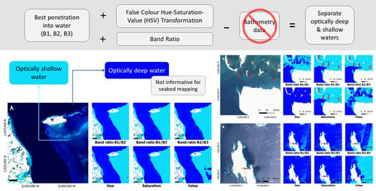For brevity, only the L1C classification maps are displayed and readers are referred to the Appendix A Figure A1, Figure A2, Figure A3 and Figure A4 for the L2A classification maps.

The optimal waters of the Bahamas allowed all bands to perform quantitatively well, even for values whose metrics outperformed saturation in the L1C product but had a worse classification map (Figure 9). The B1/B2 band ratio performed best in these clear waters, too, with the Cross PAUA method achieving a mean OA of 0.98 ± 0.00 and the Best OA method of 0.99 ± 0.00 for the L1C product, in comparison with its relatively worse performance among the band ratios in all other sites with their less optimal environmental conditions. Nonetheless, B1/B2 had the best classification map here with the least under- or overcommission.

In the more turbid waters of the Caspian Sea and Wadden Sea, the B2/B3 band ratio was the best band combination (Figure 10 and Figure 11). There is a contrasting quantitative performance between hue and saturation for both products using the Cross PAUA method, which translated into an inversed map (Figure 11). This is reflected in the very low OA and F1 scores and most evidently in the highly negative MCC scores (Figure 7 and Figure 8), suggesting that the MCC can better highlight potential inversion with a lack of relationship at 0 instead of 50. In particular, the lack of an inversed map for the Best OA method (Figure 10) when compared to the cross PAUA method suggests that minimising estimation errors during training would produce better results than merely focusing on the best overall accuracy.

In the sunglinted waters of Tanzania, the B2/B3 band ratio was the best for the L1C product with a mean OA of 0.81 ± 0.04 using the best OA method, while saturation had a corresponding value of 0.77 ± 0.04. For the L2A product, hue was the best at 0.87 ± 0.03 using the best OA method while the B1/B3 band ratio was the best band ratio at 0.87 ± 0.03 by preserving more shallow water pixels than the B2/B3 band ratio. Notably, the sunglint and Sentinel-2 parallax effect posed a challenge, with noise in the eastern waters in the B1/B3 band ratio as well as saturation and distinct overcommission of sunglinted pixels along the parallax strips in the other indices (Figure 12). This parallax effect is also subtly present in the Bahamas, such as the diagonal noise patterns in the B2/B3 band ratio classification map (Figure 9).

3.2. Performance Comparison between Threshold Methods

The Best OA and Cross PAUA method had similar performances of mean OA that were usually above 0.70, and their recommended threshold values are very close. While the Cross PAUA method has an edge when considering the inversed maps as shown in Section 3.1, the Best OA method allows for other bands to produce a consistently better mean OA in almost all sites.

Comparatively, more of the unsupervised method’s mean OA scores were below 0.80. As an unsupervised method, the Otsu’s selected threshold remained constant throughout the k-fold. Yet, it yielded larger errors of margin for the confidence intervals of the various metrics than the corresponding results of the Best OA and Cross PAUA in the Wadden Sea (Figure 7). While this implies that the k-fold is successful in producing different training and validation datasets, the unsuitability of the Otsu’s method for these spectral indices is also highly evident.

4. Discussion

This study explores the potential of using different spectral features from another colour space to differentiate between optically deep and optically shallow waters. This is less commonly looked into since many studies are generally focused at shallower depths to reduce or avoid uncertainty errors [26,27]. As purely spectral methods, the band ratios and false colour HSV-transformed bands provide a user-friendly option to mask out deep waters.

4.1. Atmospheric Correction and Its Interaction with HSV

Interestingly, no additional atmospheric or water column correction is required before the masking process. This is atypical for coastal remote sensing [3] but not without precedent [16,45]. On the other hand, the lack of atmospheric correction would lead to a classification that is more susceptible to environmental conditions. Sunglinted and turbid pixels as well as pixels lying in the brighter parallax stripes might introduce underestimations in depth [6,54]. Furthermore, the parallax effect is especially apparent over the non-Lambertian sea surface [54], and some noise is currently recalcitrant despite a morphological filter. Thus, this study is not advocating for disregarding atmospheric correction altogether. Regardless, this approach is transferable to other sites, since the optical properties of water are generally similar in the tropical and temperate coastal aquatic regions [55].

The finding that the bottom of atmosphere L2A images work better with hue might explain the prominence of true colour hue in ocean colours of different sensors [6,37,56] over saturation. Many of these studies are more interested in the water colour or water column signals, while our study is on the substratum or benthic seabed signal. Thus, this suggests possibilities in form of alternative band combinations that are suitable for different purposes or even in different types of aquatic environments such as rivers.

4.2. Comparison with Systematic Optimisation

Since this study showed that different band pairs perform best at different sites, it would logically follow that a systematic optimisation approach such as OBRA, MODPA or SMART-SDB would provide competitive performances. This is in line with Lee et al. [16], who found that the R_rs of shallow waters are governed by multiple variables and no single band ratio can account for all these variations. However, owing to a lack of normalisation and the potential for overcorrection to produce extreme values, the dynamic ranges of band ratios need to be managed. The computational demand might be greater if the optimisation search algorithm is iterative and reliant on the range itself [29]. Regardless, the optimisation approaches are still available to users.

4.3. Thresholding

While the boundary between both classes might not align with the bathymetric contours, owing to possible heterogeneity across the images as well as between different seabed covers [57], the supervised methods proved its possibility. Unfortunately, the selected unsupervised method was not compatible with this application. Beyond Otsu’s method, alternative possibilities could be explored, such as the recent development of a transferable SDB approach based on multitemporal compositing and a semi-analytical model that is currently restricted to clearer waters [15], feature subspace methods to separate between different spectral clusters before applying spectral models to obtain the classification [26,45], other adaptive threshold techniques, as well as object-based image analysis [7,58]. The development on another suitable automated thresholding approach would greatly assist this HSV approach and other indices.

5. Conclusions

While an uncommon approach, hue has been previously established to identify different optical water types, as well as vertical variations in the water column. The current usage relies on original or reconstructed true colour images from remote sensing reflectance. In comparison, this study showed the viability of a 1-2-3 false colour-derived saturation and hue band to separate the optically deep and shallow waters in Sentinel-2 L1C and L2A images, respectively, over four wide-ranging tropical and temperate water quality environments without any additional atmospheric correction or bathymetry data.

Both the band ratios and 1-2-3 false colour HSV bands were able to separate optically deep and shallow waters using a supervised threshold. While some of the band ratios might have a slightly better performance quantitatively than the HSV bands, their individual performances are highly reliant on the water quality and, by extension, location. In comparison, the hue and saturation bands have a greater tolerance to more water types and are easily transferable to other sites or regions with minimal finetuning. Therefore, they show more consistency in performance and do not require optimisation. The current lack of an unsupervised adaptive threshold necessitates additional experimentation to improve its automation, scalability and effectiveness. GEE offers a computationally efficient environment for application and scalability of the HSV features across a wide range of spatial scales and coastal aquatic remote sensing applications using open and dense satellite time series, including turbidity and SDB estimations, and benthic habitat mapping.