A Comparison of Sporadic-E Occurrence Rates Using GPS Radio Occultation and Ionosonde Measurements

Abstract

Sporadic-E ($E_s$) occurrence rates from Global Position Satellite radio occultation (GPS-RO) measurements have shown to vary by a factor of five between studies, motivating the need for a comparison with ground-based measurements. In an attempt to find accurate GPS-RO techniques for detecting $E_s$ formation, occurrence rates derived using five previously developed GPS-RO techniques are compared to ionosonde measurements over an eight-year period from 2010–2017. GPS-RO measurements within 170 km of a ionosonde site are used to calculate $E_s$ occurrence rates and compared to the ground-truth ionosonde measurements. The techniques are compared individually for each ionosonde site and then combined to determine the most accurate GPS-RO technique for two thresholds on sporadic-E intensity: no lower limit and fbEs $\ge 3$ MHz. Overall, the Yu$S_4$ method shows the closest agreement with ionosonde measurements for total $E_s$ occurrence rates without a lower limit on intensity, while the phase-based Chu technique shows the closest agreement for fbEs $\ge 3$ MHz. This analysis demonstrates that the variation in GPS-RO derived sporadic-E occurrence rates is due to varying thresholds on the sporadic-E intensities in terms of fbEs.

1. Introduction

Ionospheric conditions are important to a range of electromagnetic spectrum operations including satellite and High Frequency (HF) communications. Abnormalities such as sporadic-E ($E_s$) can cause degradation of the communication signals as well reflect it entirely [1,2]. Radar techniques such as over-the-horizon-radar [3] are also significantly affected by the presence of sporadic-E, motivating the need for accurate global occurrence rates (ORs).

Sporadic-E manifests itself as a non-uniform, wavy layer, or a composition of irregular elongated clouds of intense ionization within the lower E-region of the ionosphere [1,4]. There are many methods and instruments used to monitor sporadic-E including incoherent scatter radars (ISRs) [5], ionosondes [6,7,8,9,10], and GPS radio occultation (RO) [11,12]. While ISR measurements provide detailed $E_s$ observations, the number of sites across the globe are significantly lacking for global climatological studies. Ionosondes provide robust $E_s$ measurements and include a near global coverage [13], but there are many locations with missing data such as the African sector or over the oceans. An updated global climatology for foEs and fbEs ORs was recently provided in Ref. [14], highlighting the capabilities as well as the spatial gaps arising from the strict use of ionosonde data for a global climatology.

GPS-RO provides a unique capacity for developing global $E_s$ occurrence rate climatologies. For example, the Constellation Observing Satellite for Meteorology, Ionosphere, and Climate (COSMIC-1) constellation consisted of six satellites with circular orbits at altitudes of 800 km at an inclination of 72 degrees, providing an average of 1500–2000 GPS-RO profiles per day with near global coverage [15,16]. The original COSMIC-1 constellation was recently succeeded by the COSMIC-2 constellation which increased the frequency and range of the sensors activity [17]. Using low Earth orbit (LEO) satellites to receive dual $L_1$ (1575.42 MHz) and $L_2$ (1227.60 MHz) GPS signals allows for measurements of amplitude and phase perturbations caused by a sporadic-E layers [12,18,19,20]. GPS-RO can also be used to find temperature, water vapor pressure, and ionospheric electron density [20,21]. The large number of daily GPS-RO measurements provides a unique opportunity to develop global climatologies for sporadic-E occurrence [22,23] and intensity [12,24].

While GPS-RO measurements provide nearly complete global coverage, there are large discrepancies in ORs between different GPS-RO methods for monitoring sporadic-E. For example, Ref. [22] shows a maximum $E_s$ occurrence rate of ∼10% while Ref. [23] presents a ∼50% maximum. Neither study mentions a plasma intensity threshold for the sporadic-E layer, which is likely the primary cause of the significant difference in the ORs. To anchor the different techniques to specific $E_s$ intensity thresholds, they should be compared against more direct $E_s$ measurements such as those obtained by ionosondes. This is the primary motivation behind the present research effort.

In the search for accurate GPS-RO methods for estimating sporadic-E ORs associated with fbEs $\ge 3$ MHz and for all fbEs measurements without a lower limit on intensity, five GPS-RO techniques [22,23,24,25,26] are compared to ionosonde measurements over an eight year period between 2010 and 2017. For this comparison, data from the digital ionosonde brand Digisonde as presented in Ref. [14] are used as the ground-truth for sporadic-E ORs across the globe. Two techniques will be recommended for use in estimating $E_s$ ORs for the two intensity thresholds. These techniques can be used for future climatological studies with specific intensity thresholds in mind.

2. Methods

Here we briefly outline the five GPS-RO techniques used to calculate sporadic-E ORs. To improve readability, we refer to the methods as Chu for Ref. [22], Arras for Ref. [23], Yu for Ref. [24], Niu for Ref. [25], and Gooch for Ref. [26].

Table 1. A summary of the binary sporadic-E criteria for each of the five GPS-RO techniques.

Technique	Criteria
Arras	$L_1$ SNR standard deviation greater than 0.2
Niu	Maximum TEC perturbation gradient ($S_{max}$) greater than 0.12 TECU/km
Chu	(1) $L_1$ and $L_2$ phase perturbation greater than 5 cm
	(2) Ratio of $L_1$ and $L_2$ within $\left[1.2,1.9\right]$
	(3) Amplitude of normalized $L_1$ SNR perturbation greater than 0.01
Yu	Maximum $L_1$ $S_4$ greater than 0.66
Gooch	fbEs calculated from TEC perturbation and 170 km effective
	sporadic-E length greater than 3 MHz

provides a summary of the criteria used in each technique. The GPS-RO data used in this analysis was obtained from the COSMIC Data Analysis and Archive Center (CDAAC, https://cdaac-www.cosmic.ucar.edu/, accessed 1 September 2020).

Tangent point altitudes of 70–130 km, typical for sporadic-E, are analyzed globally to search for binary (present or not-present) $E_s$ observations. While the Arras and Chu techniques provide explicit binary criteria for $E_s$ presence, the Niu, Gooch, and Yu methods are used to estimate peak $E_s$ plasma frequencies. Then, the peak $E_s$ plasma frequencies are compared against predefined intensity thresholds used as the binary criteria for the existence of $E_s$. Here, we use a lower intensity threshold of 3 MHz and an upper threshold of 20 MHz to remove unrealistic or noisy data. While a peak $E_s$ plasma frequency threshold of 3 MHz was used for the various GPS-RO techniques, the occurrence rate results were compared to two separate ionosonde fbEs thresholds: fbEs $\ge 3$ MHz and no lower limit for a total occurrence rate. In this study, we use foEs and fbEs interchangeably for the GPS-RO techniques that provide an foEs estimate through previous comparison with ionosonde measurements. However, it must be noted that the continuous blanketing sporadic-E layers causing large GPS-RO perturbations are most likely related to fbEs rather than patchy foEs measurements [23,27] and fbEs ≤ foEs by definition. Therefore, the 3 MHz foEs thresholds used for some of the GPS-RO methods outlined below correspond to fbEs ≤ 3 MHz. As the ionosonde measurements are able to distinguish between foEs and fbEs, the ionosonde data strictly uses fbEs for this comparison.

2.1. Arras Method

The Arras method analyzes 50 Hz $L_1$ amplitude data (atmPhs files from CDAAC) in the altitude range of 70–130 km following the boundaries of typical sporadic-E. $L_1$ data is used since the lower frequency $L_2$ is noisier from elevated index of refraction gradients. To search for sporadic-E, the $L_1$ signal-to-noise ratio (SNR) is normalized and a rolling standard deviation is calculated using a 2 km window. The binary $E_s$ criteria is satisfied if the standard deviation exceeds an empirically determined value of 0.2. With typical sporadic-E vertical thicknesses on the order of 1 km [19], if the altitude extent of the perturbed region with a standard deviation over 0.2 exceeds 10 km, then the occultation is removed for quality control.

2.2. Niu Method

Total electron content (TEC) profiles are calculated using $L_1$ and $L_2$ excess phase data from CDAAC’s 1 Hz ionPhs files. The TEC profiles with an altitude range of 70–130 km are detrended using a Savitzky–Golay [28] 11-point, 3rd order polynomial to obtain the background TEC profile, ${\mathrm{TEC}}_{\mathrm{Background}}$:

$$\mathsf{\Delta }\mathrm{TEC}={\mathrm{TEC}}_{\mathrm{r}}-{\mathrm{TEC}}_{\mathrm{Background}},$$

(1)

where ${\mathrm{TEC}}_{\mathrm{r}}$ is the raw relative TEC and $\mathsf{\Delta }\mathrm{TEC}$ is the TEC perturbation (or detrended TEC). The $S_{max}$ is the maximum vertical gradient of $\mathsf{\Delta }\mathrm{TEC}$, as described by

$$S=\frac{d\left(\mathsf{\Delta }\mathrm{TEC}\right)}{dh},$$

(2)

where $dh$ is the change in altitude used to calculate the vertical TEC gradient [25]. Averaging the four linear fits of $S_{max}$ as a function of foEs obtained by Ref. [25] provides an estimate for a global linear fit:

$$S_{max}\left[\mathrm{TECU}/\mathrm{km}\right]=0.05\times foEs\left[\mathrm{MHz}\right]-0.03.$$

(3)

From this averaged slope, we find a threshold $S_{max}$ of 0.12 TECU/km corresponding to a 3 MHz foEs.

2.3. Chu Method

The 1 Hz ionPhs phase and SNR data is used within an altitude range of 70–130 km. This method requires three criteria to be satisfied simultaneously: First, both the $L_1$ and $L_2$ SNR and excess phase are smoothed with a 3-point Savitzky–Golay filter. Both the $L_1$ and $L_2$ phase perturbation magnitudes must be larger than 5 cm. The excess phase on both the $L_1$ and $L_2$ are detrended using a Savitzky–Golay filter with a 25 km window and 3rd order polynomial to remove large scale variations in the E-layer of ionosphere. The phase perturbation magnitudes, $\mathsf{\Delta }L$, are inversely proportional to the signal frequency, f, squared:

$$\mathsf{\Delta }L=\frac{40.323}{f^2}\mathsf{\Delta }\mathrm{TEC}.$$

(4)

Therefore, the ratio of $\mathsf{\Delta }{L}_2/\mathsf{\Delta }{L}_1$ should have a value of 1.65 if the signals share the same group path. From this, the second criteria requires the phase perturbation ratio to lie within the range of $\left[1.2,1.9\right]$. Note that we extended the phase perturbation ratio from the $\left[1.5,1.8\right]$ range provided by Ref. [22] to increase ORs. Finally, the amplitude of the normalized $L_1$ SNR perturbation has to be greater than 0.01. The height where the peak of the perturbation occurs is the height of the sporadic-E layer.

2.4. Yu Method

From the 50 Hz atmPhs $L_1$ SNR data, a 50-point window of (25 below and above) is used to calculate a 1 Hz $S_4$. This $S_4$ is calculated as a function of altitude and is converted to an foEs following:

$${(foEs-1.2)}^2=13.62\times S_{4,Max},$$

(5)

where $S_{4,Max}$ is the maximum of the $S_4$ index and the foEs is the peak frequency of the sporadic-E cloud. For the current study, we use a perturbation of $foEs-1.2=3.0$ MHz, following a fo$\mu$Es threshold of 3 MHz for an average background E-layer frequency of 1.2 MHz [29]. This corresponds to an $S_{4,Max}$ threshold of 0.66 to indicate a sporadic-E layer with sufficient intensity for the current comparison. It must be noted that we calculate the $S_4$ index directly from 50 Hz $L_1$ SNR data using a rolling 50 point window. This may provide slight differences to the $S_4$ values obtained directly from CDAAC [30], especially for strongly scintillating layers.

2.5. Gooch Method

Using the 50 Hz atmPhs excess phase data, a relative ${\mathrm{TEC}}_{\mathrm{r}}$ is calculated using

$${\mathrm{TEC}}_{\mathrm{r}}=\frac{1}{40.3}\frac{f_1^2{f}_2^2}{f_1^2-f_2^2}(\mathsf{\Delta }{L}_1-\mathsf{\Delta }{L}_2),$$

(6)

where $\mathsf{\Delta }{L}_1$ is the excess phase for $f_1=1.57542$ GHz and $\mathsf{\Delta }{L}_2$ is the excess phase for $f_2=1.22760$ GHz [11]. Afterward, the TEC is detrended using a Savitzky–Golay filter with a 25 km window to obtain the TEC perturbation $\mathsf{\Delta }\mathrm{TEC}$. Finally, the $\mathsf{\Delta }\mathrm{TEC}$ is smoothed using another Savitzky–Golay filter with a 1 km window. From this, the electron density is calculated by

$$\mathsf{\Delta }{n}_e=\frac{\mathsf{\Delta }\mathrm{TEC}}{2\sqrt{2R\mathsf{\Delta }R}},$$

(7)

where the TEC perturbation is divided by an effective path length of 176 km corresponding to an effective path through a cylinder with a vertical thickness of $\mathsf{\Delta }R=0.6$ km located at a radial distance R from the center of Earth [26]. The effective path length is derived from an assumed geometry of a cylinder centered around the tangent point [31]. The binary $E_s$ criteria is satisfied if the plasma frequency associated with $\mathsf{\Delta }{n}_e$ is ≥3 MHz and the detrended TEC perturbation occurs within a 10 km altitude window.

2.6. Ionosonde Measurements

Occurrence rates based on ionosonde measurements are used as the ground-truth in this comparison. A detailed explanation of the techniques used to calculate the ionosonde based ORs is outlined in Ref. [14]. In summary, ionogram-derived $E_s$ parameters were obtained from the Global Ionospheric Radio Observatory (GIRO) network of Digisondes [13] using the GIRO web portal (http://giro.uml.edu/didbase/scaled.php, accessed 26 September 2020). To ensure the most up-to-date automatic scaling processes used to determine the sporadic-E parameters, only ionograms processed with the ARTIST-5 software [32] are used to calculate ORs.

A vital distinction between foEs and fbEs must be defined when comparing GPS-RO measurements to ionosonde measurements, as the ORs can vary by a factor of five depending on the sporadic-E intensity threshold of interest [14]. Here, we assume that the fbEs layers are most likely to be measured by GPS-RO techniques because of the greater phase contribution from a continuous layer rather than the patchy foEs layers, and we compare the RO measurements to fbEs. Additionally, an intensity threshold for the sporadic-E must also be defined before comparison. In this study, we use the total sporadic-E occurrence rate as measured by ionosondes and a separate comparison for fbEs $\ge 3$ MHz. For the total occurrence rate, there is no lower limit to the sporadic-E fbEs intensity, except for the natural lower limit of ∼1.5 MHz for most ionosonde sites due to frequency allocation and sensitivity issues.

2.7. Comparison Criteria

Occurrence rates are calculated by dividing the number of sporadic-E measurements by the total number of measurements within a certain time period. For example, the ionosonde based OR for fbEs $\ge 3$ MHz is calculated by

$$OR(fbEs\ge 3\mathrm{MHz})=\frac{N(fbEs\ge 3\mathrm{MHz})}{N_{CS}},$$

(8)

where $OR(fbEs\ge 3\mathrm{MHz})$ is the occurrence rate for fbEs greater than or equal to 3 MHz, $N(fbEs\ge 3\mathrm{MHz})$ is the number of fbEs measurements during the time period of interest (seasonal or entire year) above the 3 MHz threshold, and $N_{CS}$ is the total number of vertical ionograms provided by the number of confidence scores [14]. Every ARTIST-5 scaled ionogram has an associated confidence score, so $N_{CS}$ is used as the total number of ionosonde measurements. No threshold is placed on the ionogram-derived confidence scores for this analysis.

A similar method is used for the GPS-RO derived ORs, except a measurement area around each ionosonde is used to calculate the rates. The measurement area corresponds to circles centered around the Digisonde sites with radii of 170 km, corresponding to the mean length of sporadic-E [33]. A map of the measurement areas used in this analysis are displayed in Figure 1. Ionosonde and RO based ORs were compared seasonally near the same location to ensure a direct comparison. The comparison is performed for each season with ORs averaged over the years 2010–2017. This time period was selected to ensure sufficient ARTIST-5 scaled Digisonde and COSMIC-1 data was available simultaneously.

To maximize the number of data points, ORs were not separated by time of day (TOD) and the values provided here correspond to all-day averages. A quality control check was placed on the data using the technique outlined in Ref. [34], which places an upper limit of 1.5 on the mean deviation of the electron density (or here, TEC) profile. GPS-RO profiles with few data points (less than 400 for the 50 Hz data) were also excluded from the analysis. Ionosonde sites were required to have >4320 ionograms for the season of interest in a given year to be included in the comparison. This corresponds to ionosonde operation roughly half of the season assuming a 15 min ionogram cadence [14]. The seasonal results throughout 2010–2017 are combined to perform the statistical comparison between GPS-RO and ionosonde derived ORs. A lower limit of 10 observations was placed on the GPS-RO data at each site to be included in the combined data set for seasonal comparisons. Temporal gaps in ionosonde operations combined with quality control checks of the GPS-RO data [34] create a variable number of sites with an amount of GPS-RO observations greater than 10 (which is the lower limit for which the comparison is made) in the different seasons (i.e., summer and winter as discussed below).

Instead of directly comparing ionograms and GPS-RO crossings within a short time window (e.g., 30 min between ionogram and crossing as outlined in Ref. [26]), here we compare rates averaged over TOD for the areas surrounding each ionosonde site. A direct comparison of each GPS-RO crossing within 170 km of a site certainly has merit as it ensures the measurements are taken at nearly the same time and location. However, due to the patchy nature of $E_s$ clouds, simultaneous ionosonde and GPS-RO measurements can sample different parts of the cloud and provide varying results (see the discussion in Ref. [26]). As an alternative approach, here we use all Digisonde measurements at a particular site over a season to calculate the OR averaged over TOD. Then, as the GPS-RO measurements randomly sample the area surrounding the Digisonde site over all local times, the TOD averaged results from the GPS-RO rates should align with the TOD averaged Digisonde rates if the GPS-RO techniques properly characterize the existence of $E_s$ layers. A large number of ionosonde measurements are taken over a season, which provides a robust TOD average over the site of interest. While this statistical comparison would be flawed if the number of GPS-RO crossings is very low and clustered around a particular TOD, a larger number of measurements spread throughout TOD provides a proper sampling around the site such that the rates can be compared with the ionosonde rates. As described later, the average number of GPS-RO observations within 170 km of each site over all seasons and years is greater than 100 (

Table 2. Average number of ionosonde and GPS-RO observations over each site for all seasons and years.

Technique	Average Number of Observations	Average Number of ${\mathrm{E}}_{\mathrm{s}}$ Observations	Ratio
Ionosonde	249,524	—	—
(1) no fbEs limit	—	39,485	0.16
(2) fbEs $\ge 3$ MHz	—	19,546	0.08
Arras	156	42	0.27
Gooch	156	42	0.27
Yu	156	22	0.14
Chu	118	9	0.08
Niu	118	28	0.24

) and the average number of ionosonde observations is over 200,000, providing a measure of confidence in the statistical results through proper sampling over the TOD for both ionosonde and GPS-RO derived rates.

3. Results

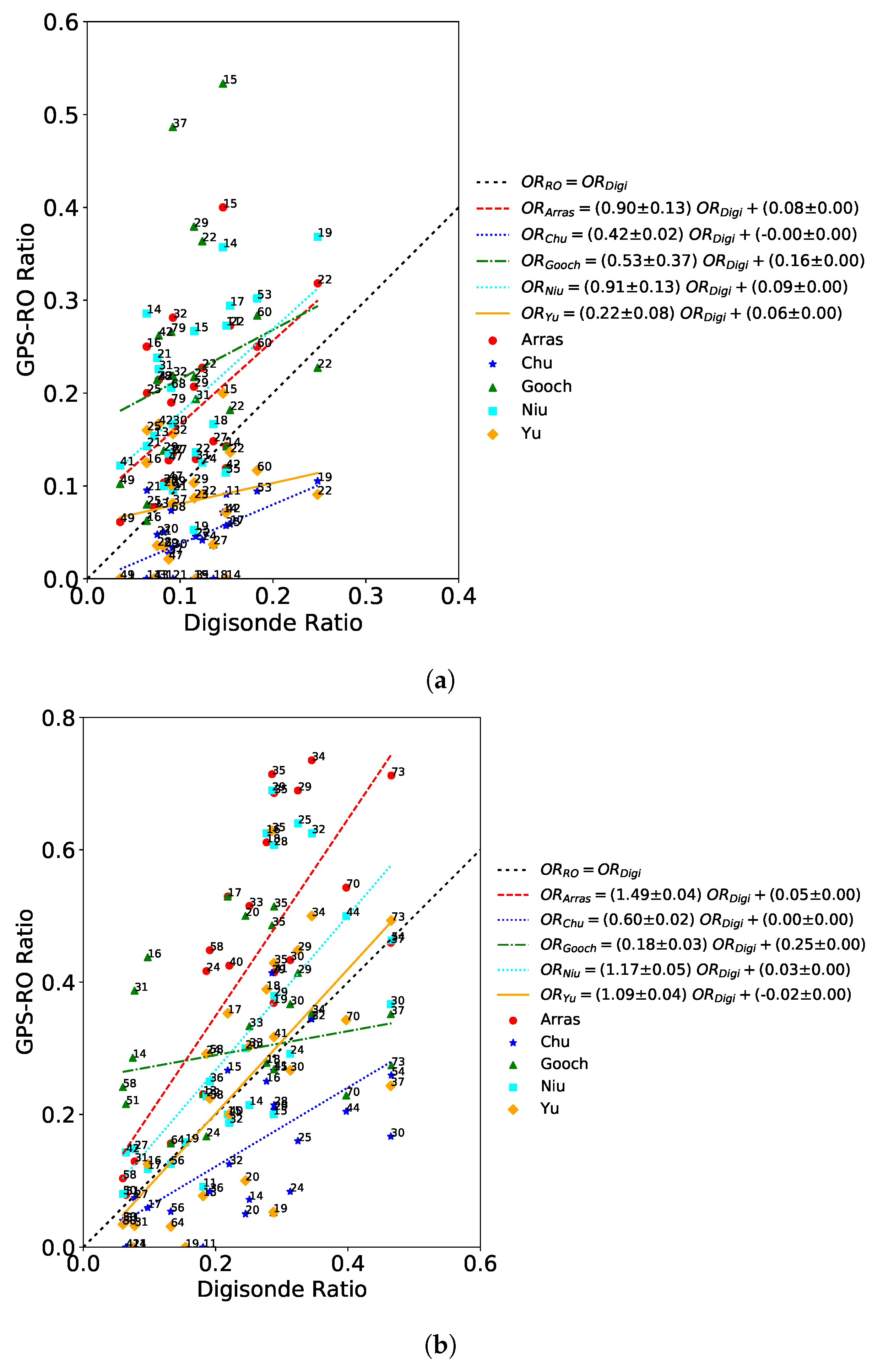
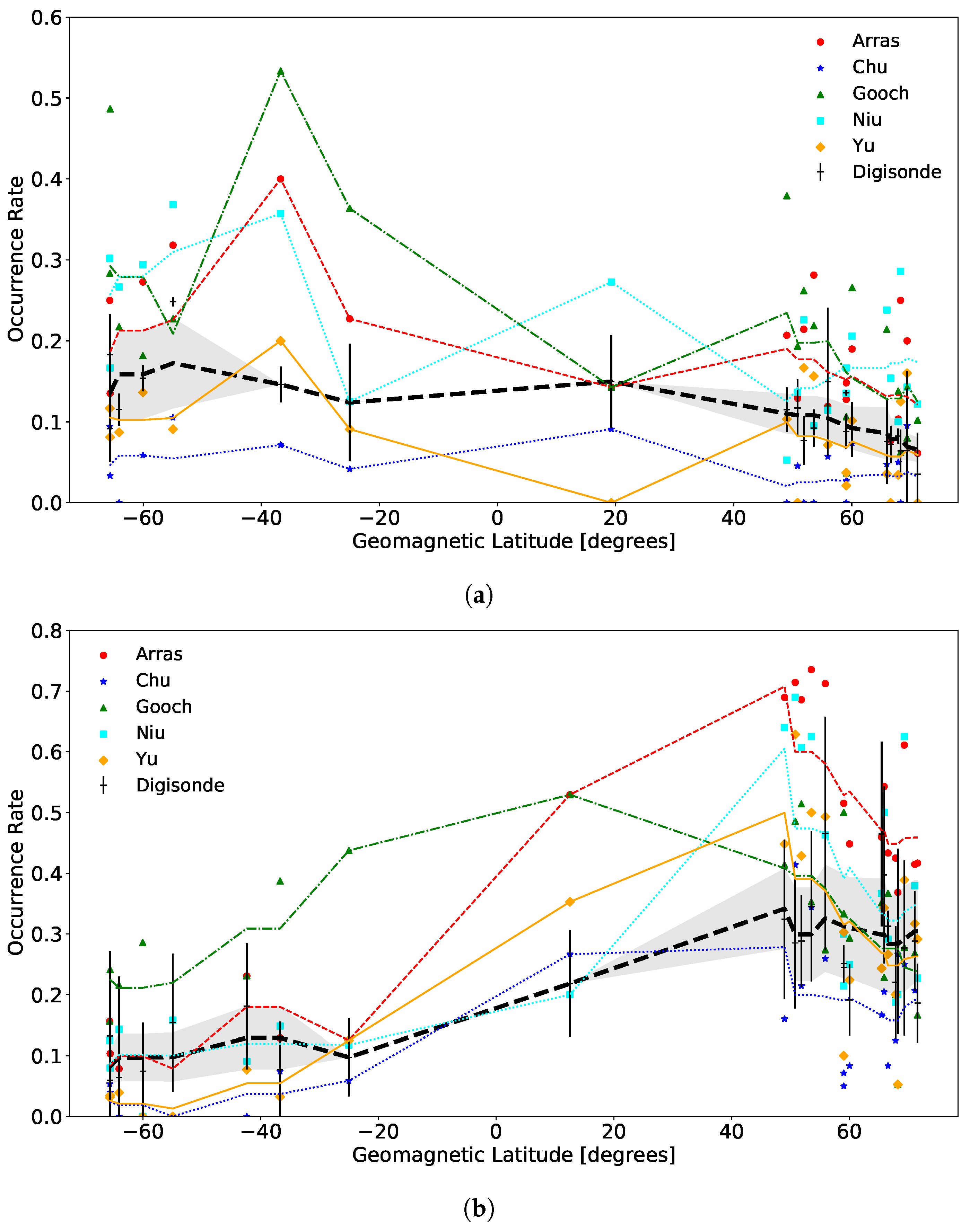
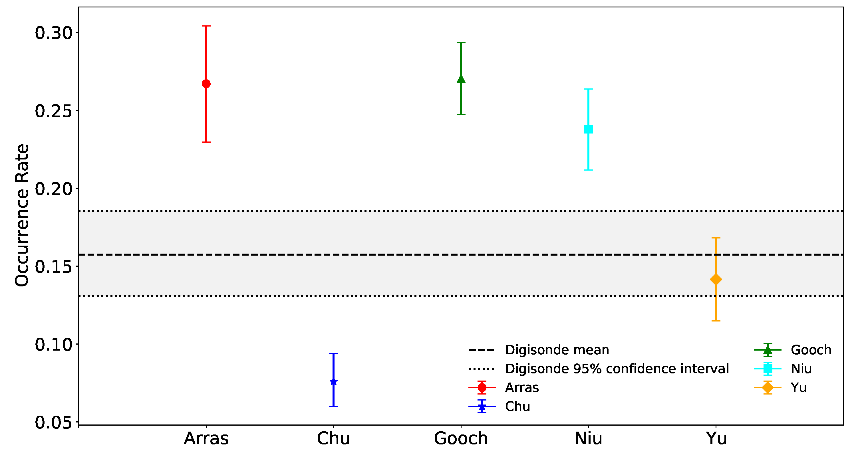
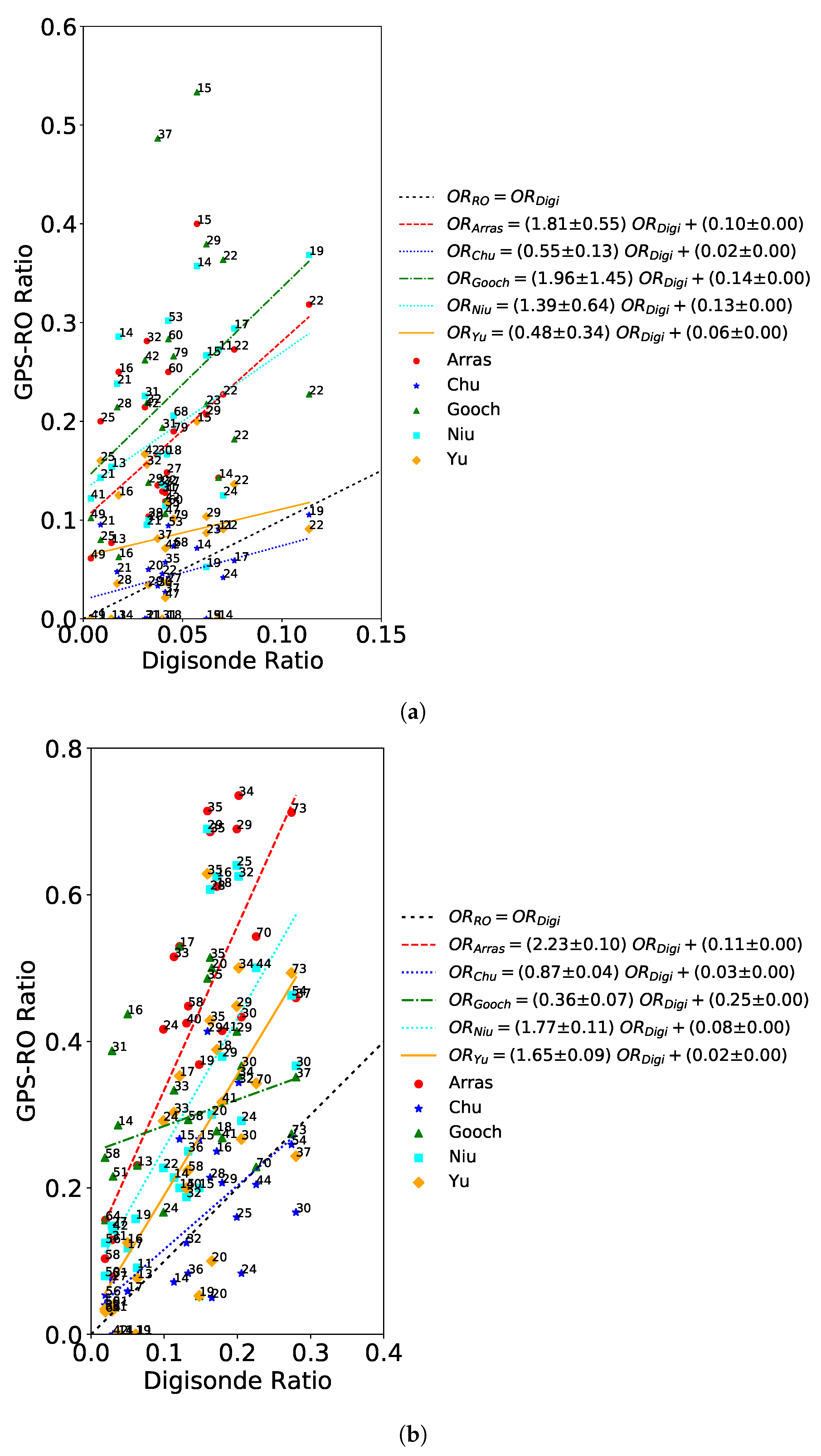
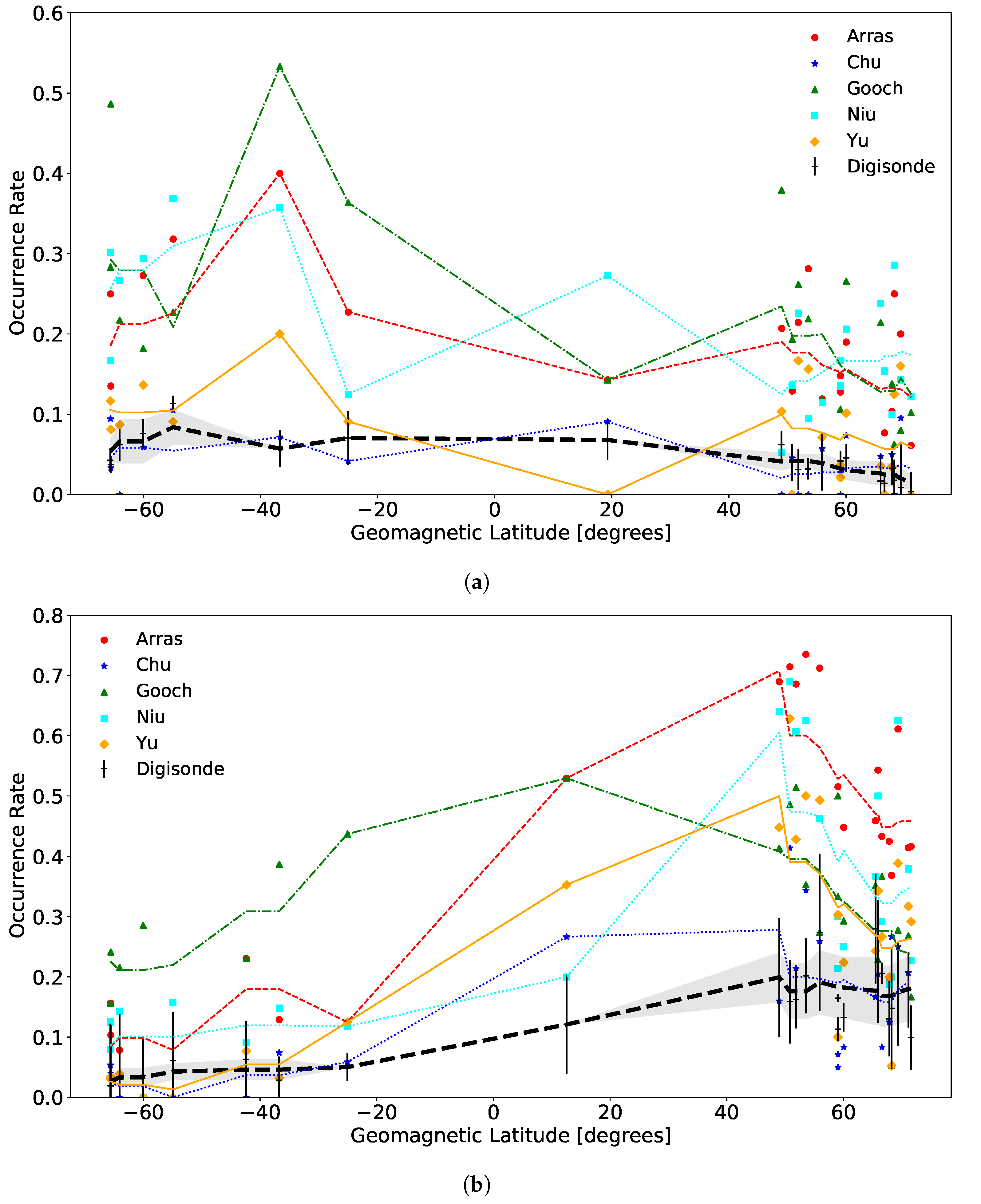
3.1. No Lower fbEs Limit

The GPS-RO and Digisonde derived ORs were compared over all seasons, but here we show only the summer and winter results for brevity. Figure 2 displays the results for the five RO techniques calculated over each Digisonde site in comparison to the ionosonde-derived total sporadic-E ORs with no lower limit on fbEs intensity. The number of ionosonde sites satisfying the threshold of at least 10 GPS-RO measurements varies between seasons with 22 sites for December–February and 25 sites for June–August. This difference in number of sites is due to temporal gaps in ionosonde operations combined with quality control of GPS-RO data, and sites with ≤10 GPS-RO crossings are removed from the comparison. Comparisons over all seasons (entire year) include the 30 sites displayed in Figure 1. The number of GPS-RO crossings within 170 km of each Digisonde site are annotated in Figure 2 to display the combined number of GPS-RO measurements used to calculate $E_s$ ORs over each ionosonde site for the season of interest during 2010–2017.

A linear regression of the GPS-RO derived ORs with respect to the ionosonde ORs is calculated for each method using a bootstrapping technique with 10,000 resamples. The bootstrapping technique allows for estimation of a statistical parameter through random resampling of the original dataset with replacement (random selection from the original data points), allowing for a quantification of the uncertainty in a statistical parameter of interest [35]. Here, the mean linear regression coefficients (slope and intercept) and associated variance are estimated for each GPS-RO method with respect to the ionosonde ORs. The linear fit provides a measure of the general trend and should be compared against the one-to-one line (slope = 1, intercept = 0) that indicates a perfect match between data sets with equal ORs for the GPS-RO and ionosonde measurements. Differences between the estimated ORs can manifest as a difference in slope (GPS-RO and ionosonde rates not increasing at the same rate) or in magnitude (GPS-RO underestimates or overestimates the magnitude relative to the ionosonde rates). In the boreal winter season, the Gooch (green) and Niu (cyan) techniques overestimate the ORs. However, the slope of the two methods correlates to the ionosonde ratios. The Arras (red) method slightly overestimates the slope and OR magnitudes. The Chu (blue) methodology underestimates both the ORs and slope. The Yu (yellow) method crosses the one-to-one line, but the slope is less than one which would increase the gap between the ionosonde ratios for larger ORs. In the boreal summer season, the Chu method underestimates and the Arras and Niu methods overestimate the rates. The Gooch technique crosses the one-to-one lines but the slope is much less than one. Here, the Yu technique closely matches both the slope and OR magnitudes.

Figure 2 also shows the variance of the linear regression coefficients. For boreal winter, the Gooch technique shows a relatively large variance of 0.37 for the slope while the Chu technique displays a small variance of 0.02. The slope variances are reduced for boreal summer, all ≤0.05. The intercept coefficients range from 0.25 for the Gooch method in boreal summer to 0.00 for the Chu method. The variance in intercepts are all 0.00.

The ORs as a function of geomagnetic latitude are displayed in Figure 3 for winter and summer. Rolling spatial averages are calculated for each GPS-RO technique and ionosonde-derived values using a $\pm {10}^{\circ }$ window to estimate trends as a function of geomagnetic latitude. Ionosonde error bars are presented at each site from standard deviations calculated over the range of years. Additionally, the shaded region around the ionosonde trendline (dashed black line) represents a rolling spatial standard deviation calculated using a $\pm {10}^{\circ }$ latitude window.

The expected latitude dependence of sporadic-E formation is immediately obvious, with a maximum in the local summer hemisphere much larger than the ORs in the local winter hemisphere. This result is in agreement with many previous studies [36,37,38]. In the boreal winter, the Arras and Gooch techniques overestimate rates while the Niu technique overestimates at all latitudes except one. In general, the Yu technique slightly underestimates the values except for a couple of latitude positions, and the Chu technique underestimates for all latitudes. Overall, the Yu technique shows the closest agreement with the ionosonde results for the boreal winter. For the boreal summer season, most GPS-RO techniques align with the ionosonde rates over some range of latitudes. In general, the Arras and Gooch techniques overestimate the ORs, but the Chu, Yu, and Niu techniques all show reasonable agreement overall.

To compare the various RO techniques to the ionosonde results over all seasons and years, a bootstrap calculated mean using 10,000 random resamples with replacement from the original dataset was calculated for each method (Figure 4). These results show that the Yu technique most closely aligns with the mean ionosonde ORs without a lower threshold on fbEs intensity, while the Chu technique underestimates and the Gooch, Arras, and Niu techniques overestimate. Similarly, the ORs averaged over all sites, seasons, and years, as displayed in Table 2, show an average of 14% for the Yu technique and an ionosonde average of 16%. Finally, statistical similarity is calculated as the percentage of overlap between uncertainty intervals calculated for a particular statistical metric. For the occurrence rate means, the statistical similarity is displayed in

Table 3. Digisonde and GPS-RO mean statistical similarity for no lower limit on $E_s$ intensity. Bold values highlight the largest statistical similarity for each season.

Technique	Dec.–Feb.	Mar.–May	Jun.–Aug.	Sep.–Nov.	Entire Year
Arras	0.01	0.00	0.12	0.03	0.00
Chu	0.00	0.00	0.02	0.04	0.00
Gooch	0.00	0.00	0.85	0.00	0.00
Niu	0.00	0.00	0.68	0.01	0.00
Yu	0.29	0.57	0.67	0.21	0.57

. As highlighted by the bootstrapping results (Figure 4), the Yu technique shows the most overlap and has the strongest statistical similarity with the ionosonde means overall. However, the Gooch technique shows the strongest statistical similarity in the boreal summer season, likely due to the close match in the northern midlatitudes during this period and the Yu method underestimation of the rates in the Southern Hemisphere.

3.2. fbEs $\ge 3$ MHz

The comparison is repeated for fbEs intensities greater than 3 MHz, which in general are reduced from the total sporadic-E ORs by a factor of roughly 2/3 [14]. This distinction between sporadic-E intensity is important as the GPS-RO derived ORs show relatively large variations in magnitudes between the various techniques. While the Chu technique tends to underestimate the ORs for no lower limit on $E_s$ intensity, we find a close agreement with the fbEs $\ge 3$ MHz rates derived from ionosonde measurements. Figure 5 shows a scatter plot of the winter and summer ORs for each GPS-RO technique separated by Digisonde site. As discussed in Section 3.1, there are 22 sites for December–February and 25 sites for June–August with greater than 10 GPS-RO crossings throughout 2010–2017 over the season of interest. Linear regressions and associated variances of GPS-RO rates as a function of ionosonde rates are calculated through bootstrapping. All other RO techniques overestimate the $E_s$ ORs while the Chu method shows agreement in both slope and magnitude.

Overall, the Chu technique shows the closest agreement with ionosonde rates over the range of geomagnetic latitudes, as displayed in Figure 6. While the Chu technique overestimates the OR in the equatorial region in boreal summer, there is reasonable agreement in the midlatitudes during summer and winter. In general, the other techniques tend to overestimate the rates for this fbEs threshold.

Combining the data over all sites, years, and seasons indicates a strong agreement between the bootstrap calculated means for the Chu method and the ionosonde-derived values (Figure 7). This result is also supported by the overall average of 8% taken over all sites, seasons, and years for both the ionosonde and Chu results (Table 2). Finally, the statistical similarity of 88% for the Chu technique over the entire year, as displayed in

Table 4. Digisonde and GPS-RO mean statistical similarity for fbEs $\ge 3$ MHz. Bold values highlight the largest statistical similarity for each season.

Technique	Dec.–Feb.	Mar.–May	Jun.–Aug.	Sep.–Nov.	Entire Year
Arras	0.00	0.00	0.00	0.00	0.00
Chu	0.69	0.37	0.75	0.90	0.88
Gooch	0.00	0.00	0.00	0.00	0.00
Niu	0.00	0.00	0.01	0.00	0.00
Yu	0.01	0.08	0.15	0.08	0.00

, gives confidence in using this method for characterizing sporadic-E ORs of fbEs $\ge 3$ MHz.

4. Conclusions

Five GPS-RO methods for monitoring sporadic-E occurrence rates from Refs. [22,23,24,25,26] are compared against Digisonde results obtained through the GIRO network to find techniques with strong agreement for two limits on sporadic-E intensity: no lower limit and fbEs $\ge 3$ MHz. Data over a period of 2010–2017 were analyzed and separated by season to compare the techniques’ occurrence rates. For GPS-RO techniques without binary criteria, a threshold $E_s$ layer intensity of 3 MHz was implemented to provide a binary threshold for $E_s$ occurrence. Results for the five techniques varied depending on the statistical measurement, season, and sporadic-E intensity threshold.

For the total occurrence rates with no lower limit on $E_s$ intensity, the Yu$S_4$ technique showed the closest agreement with ionosonde rates. In general, the Arras, Gooch, and Niu methods overestimated the occurrence rates for this $E_s$ intensity, while the Chu method underestimated rates. However, it must be noted that most techniques showed large variations in rates and no technique perfectly aligned with the ionosonde results over all locations and seasons. Occurrence rates calculated for fbEs $\ge 3$ MHz showed a strong agreement between the Chu technique and the ionosonde-derived rates. The other techniques overestimated the occurrence rates for this $E_s$ intensity threshold, in general.

Overall, the results of this comparison show that the many GPS-RO techniques for monitoring sporadic-E show a wide variation in occurrence rates because they ultimately map to different intensity thresholds for sporadic-E (i.e., fbEs or foEs). While the Yu technique aligns with ionosonde rates without a lower limit on fbEs and the Chu technique aligns with fbEs $\ge 3$ MHz, the other techniques likely align to various foEs thresholds with higher occurrence rates as outlined in Ref. [14]. Further research is required for these comparisons, but the key issue of understanding the large difference in GPS-RO derived sporadic-E occurrence rates has been solved.

These various GPS-RO techniques can be used to create updated global climatologies of sporadic-E occurrence for specific $E_s$ intensity thresholds. Combining GPS-RO and ionosonde data would provide a synergistic combination with nearly global coverage. Possible improvements to the various techniques, or an ensemble approach combining multiple techniques, may also help to improve the statistical similarity with ionosonde-derived occurrence rates.

References

1. Whitehead, J. Recent work on mid-latitude and equatorial sporadic-E. J. Atmos. Terr. Phys. 1989, 51, 401–424. [Google Scholar] [CrossRef]
2. Rice, D.; Sojka, J.; Eccles, J.; Raitt, J.; Brady, J.; Hunsucker, R. First results of mapping sporadic E with a passive observing network. Space Weather 2011, 9. [Google Scholar] [CrossRef]
3. Fabrizio, G.A. High Frequency Over-the-Horizon Radar: Fundamental Principles, Signal Processing, and Practical Applications; McGraw-Hill Education: New York, NY, USA, 2013. [Google Scholar]
4. Haldoupis, C. A tutorial review on sporadic E layers. In Aeronomy of the Earth’s Atmosphere and Ionosphere; Springer: Berlin/Heidelberg, Germany, 2011; pp. 381–394. [Google Scholar]
5. Mathews, J. Sporadic E: Current views and recent progress. J. Atmos. Sol.-Terr. Phys. 1998, 60, 413–435. [Google Scholar] [CrossRef]
6. Smith, E.K. Worldwide Occurrence of Sporadic E.; US Department of Commerce, National Bureau of Standards: Boulder, CO, USA, 1957; Volume 582. [Google Scholar]
7. Matsushita, S.; Reddy, C. A study of blanketing sporadic E at middle latitudes. J. Geophys. Res. 1967, 72, 2903–2916. [Google Scholar] [CrossRef]
8. Whitehead, J. The structure of sporadic E from a radio experiment. Radio Sci. 1972, 7, 355–358. [Google Scholar] [CrossRef]
9. Pignalberi, A.; Pezzopane, M.; Zuccheretti, E. A spectral study of the mid-latitude sporadic E layer characteristic oscillations comparable to those of the tidal and the planetary waves. J. Atmos. Sol.-Terr. Phys. 2015, 122, 34–44. [Google Scholar] [CrossRef]
10. Yadav, V.; Kakad, B.; Bhattacharyya, A.; Pant, T. Quiet and disturbed time characteristics of blanketing Es (Esb) during solar cycle 23. J. Geophys. Res. Space Phys. 2017, 122, 11–591. [Google Scholar] [CrossRef]
11. Hocke, K.; Igarashi, K.; Nakamura, M.; Wilkinson, P.; Wu, J.; Pavelyev, A.; Wickert, J. Global sounding of sporadic E layers by the GPS/MET radio occultation experiment. J. Atmos. Sol.-Terr. Phys. 2001, 63, 1973–1980. [Google Scholar] [CrossRef]
12. Wu, D.L.; Ao, C.O.; Hajj, G.A.; de La Torre Juarez, M.; Mannucci, A.J. Sporadic E morphology from GPS-CHAMP radio occultation. J. Geophys. Res. Space Phys. 2005, 110. [Google Scholar] [CrossRef] [Green Version]
13. Reinisch, B.W.; Galkin, I.A. Global ionospheric radio observatory (GIRO). Earth Planets Space 2011, 63, 377–381. [Google Scholar] [CrossRef] [Green Version]
14. Merriman, D.; Nava, O.; Dao, E.; Emmons, D. Comparison of seasonal foEs and fbEs occurrence rates derived from global Digisonde measurements. Atmosphere 2021, 12, 1558. [Google Scholar] [CrossRef]
15. Sharing Earth Observation Resources. FormoSat-3/COSMIC (Constellation Observing System for Meteorology, Ionosphere and Climate). 2014. Available online: https://directory.eoportal.org/web/eoportal/satellite-missions/content/-/article/formosat-3 (accessed on 6 January 2021).
16. Rocken, C.; Ying-Hwa, K.; Schreiner, W.S.; Hunt, D.; Sokolovskiy, S.; McCormick, C. COSMIC system description. Terr. Atmos. Ocean. Sci. 2000, 11, 21–52. [Google Scholar] [CrossRef] [Green Version]
17. Satellite, N.E.; Service, D. COSMIC 2. 2020. Available online: https://www.nesdis.noaa.gov/COSMIC-2 (accessed on 6 January 2021).
18. Ware, R.H.; Fulker, D.W.; Stein, S.A.; Anderson, D.N.; Avery, S.K.; Clark, R.D.; Droegemeier, K.K.; Kuettner, J.P.; Minster, J.B.; Sorooshian, S. SuomiNet: A real-time national GPS network for atmospheric research and education. Bull. Am. Meteorol. Soc. 2000, 81, 677–694. [Google Scholar] [CrossRef] [Green Version]
19. Zeng, Z.; Sokolovskiy, S. Effect of Sporadic E Clouds on GPS Radio Occultation Signals. Geophys. Res. Lett. 2010, 37. [Google Scholar] [CrossRef]
20. Chu, Y.H.; Su, C.L.; Ko, H.T. A global survey of COSMIC ionospheric peak electron density and its height: A comparison with ground-based ionosonde measurements. Adv. Space Res. 2010, 46, 431–439. [Google Scholar] [CrossRef]
21. Kursinski, E.R.; Hajj, G.A.; Leroy, S.S.; Herman, B. The GPS radio occulation technique. TAO Terr. Atmos. Ocean. Sci. 2000, 11, 53–114. [Google Scholar] [CrossRef] [Green Version]
22. Chu, Y.H.; Wang, C.; Wu, K.; Chen, K.; Tzeng, K.; Su, C.L.; Feng, W.; Plane, J. Morphology of sporadic E layer retrieved from COSMIC GPS radio occultation measurements: Wind shear theory examination. J. Geophys. Res. Space Phys. 2014, 119, 2117–2136. [Google Scholar] [CrossRef]
23. Arras, C.; Wickert, J. Estimation of ionospheric sporadic E intensities from GPS radio occultation measurements. J. Atmos. Sol.-Terr. Phys. 2018, 171, 60–63. [Google Scholar] [CrossRef]
24. Yu, B.; Scott, C.J.; Xue, X.; Yue, X.; Dou, X. Derivation of global ionospheric Sporadic E critical frequency (fo Es) data from the amplitude variations in GPS/GNSS radio occultations. R. Soc. Open Sci. 2020, 7, 200320. [Google Scholar] [CrossRef] [PubMed]
25. Niu, J.; Weng, L.; Meng, X.; Fang, H. Morphology of Ionospheric Sporadic E Layer Intensity Based on COSMIC Occultation Data in the Midlatitude and Low-Latitude Regions. J. Geophys. Res. Space Phys. 2019, 124, 4796–4808. [Google Scholar] [CrossRef]
26. Gooch, J.Y.; Colman, J.J.; Nava, O.A.; Emmons, D.J. Global ionosonde and GPS radio occultation sporadic-E intensity and height comparison. J. Atmos. Sol.-Terr. Phys. 2020, 199, 105200. [Google Scholar] [CrossRef]
27. Reddy, C.; Mukunda Rao, M. On the physical significance of the Es parameters ƒbEs, ƒEs, and ƒoEs. J. Geophys. Res. 1968, 73, 215–224. [Google Scholar] [CrossRef]
28. Savitzky, A.; Golay, M.J. Smoothing and differentiation of data by simplified least squares procedures. Anal. Chem. 1964, 36, 1627–1639. [Google Scholar] [CrossRef]
29. Haldoupis, C. An Improved Ionosonde-Based Parameter to Assess Sporadic E Layer Intensities: A Simple Idea and an Algorithm. J. Geophys. Res. Space Phys. 2019, 124, 2127–2134. [Google Scholar] [CrossRef]
30. Syndergaard, S. COSMIC S4 Data; UCAR/CDAAC: Boulder, CO, USA, 2006. [Google Scholar]
31. Ahmad, B. Accuracy and Resolution of Atmospheric Profiles Obtained from Radio Occultation Measurements. Ph.D. Thesis, Stanford University, Stanford, CA, USA, 1999; p. 1647. [Google Scholar]
32. Galkin, I.A.; Reinisch, B.W. The new ARTIST 5 for all digisondes. Ionosonde Netw. Advis. Group Bull. 2008, 69, 1–8. [Google Scholar]
33. Cathey, E.H. Some midlatitude sporadic-E results from the Explorer 20 satellite. J. Geophys. Res. 1969, 74, 2240–2247. [Google Scholar] [CrossRef]
34. Yang, K.F.; Chu, Y.H.; Su, C.L.; Ko, H.T.; Wang, C.Y. An examination of FORMOSAT-3/COSMIC ionospheric electron density profile: Data quality criteria and comparisons with the IRI model. Terr. Atmos. Ocean. Sci. 2009, 20, 193. [Google Scholar] [CrossRef] [Green Version]
35. Gareth, J.; Daniela, W.; Trevor, H.; Robert, T. An Introduction to Statistical Learning: With Applications in R; Spinger: Berlin/Heidelberg, Germany, 2013. [Google Scholar]
36. Baggaley, W. Structure in the seasonal variations of Es at southern latitudes. J. Atmos. Terr. Phys. 1986, 48, 385–391. [Google Scholar] [CrossRef]
37. Pietrella, M.; Bianchi, C. Occurrence of sporadic-E layer over the ionospheric station of Rome: Analysis of data for thirty-two years. Adv. Space Res. 2009, 44, 72–81. [Google Scholar] [CrossRef]
38. Haldoupis, C.; Pancheva, D.; Singer, W.; Meek, C.; MacDougall, J. An explanation for the seasonal dependence of midlatitude sporadic E layers. J. Geophys. Res. Space Phys. 2007, 112. [Google Scholar] [CrossRef]
Figure 1. A map of the areas around Digisonde sites corresponding to a radius of 170 km used to calculate E s occurrence rates from GPS-RO measurements. The shadowed region corresponds to ± 10 of geomagnetic latitude.
Remotesensing 14 00581 g001
Figure 2. Sporadic-E total occurrence rates for each GPS-RO technique separated by Digisonde site with no lower limit on E s intensity. Linear regressions and corresponding variances calculated using a bootstrapping technique with 10,000 samples are also displayed. The annotated numbers near each data point correspond to the number of GPS-RO observations for the season within 170 km of the Digisonde site used for comparison. The black dashed one-to-one line indicates a perfect match between data sets. Note the change in scale between the two figures and the variable number of Digisonde sites with sufficient GPS-RO crossings during the different seasons (22 sites for December–February and 25 for June–August). (a) December, January, and February 2010–2017. (b) June, July, and August 2010–2017.
Remotesensing 14 00581 g002
Figure 3. Total occurrence rates with no lower limit on E s intensity as a function of latitude with spatial rolling averages calculated using a ± 10 window for trendlines. Shading around the Digisonde trendline (black dashed line) represents a rolling standard deviation of the Digisonde ORs with a ± 10 latitude window. Ionosonde error bars are calculated from a standard deviation taken over 2010–2017 using the OR from each year as a separate data point. Note the change in scale between the two figures. (a) December, January, and February 2010–2017. (b) June, July, and August 2010–2017.
Remotesensing 14 00581 g003
Figure 4. Bootstrap calculated means and 95% confidence intervals for each GPS-RO technique compared to the ionosonde rates over all seasons and years for no lower limit on E s intensity. Each point represents the mean and confidence interval for the GPS-RO technique displayed below on the abscissa, while the dashed line and shaded region across all techniques shows the Digisonde mean and 95% confidence interval.
Remotesensing 14 00581 g004
Figure 5. Same as Figure 2, but for fbEs 3 MHz. (a) December, January, and February 2010–2017. (b) June, July, and August 2010–2017.
Remotesensing 14 00581 g005
Figure 6. Same as Figure 3, but for fbEs 3 MHz. (a) December, January, and February 2010–2017. (b) June, July, and August 2010–2017.
Remotesensing 14 00581 g006
Figure 7. Same as Figure 4, but for fbEs 3 MHz.
Remotesensing 14 00581 g007