Abstract
Rapid urban expansion and structural changes are taking place in China’s capital city, Beijing, but without an update of urban land features in a timely manner our understanding of the new urban heterogeneity is restricted, as land-background data is indispensable for bio-geophysical and bio-geochemical processes. In this plain region, the investigations of multi-scale urban land mappings and physical medium environmental elements such as slope, aspect, and water resource services are still lacking, although Beijing can provide an exemplary case for urban development and natural environments in plains considering the strategic function of China’s capital city. To elucidate these issues, a remote-sensing methodology of hierarchical urban land mapping was established to obtain the urban land, covering structure and its sub-pixel component with an overall accuracy of over 90.60%. During 1981–2021, intense and sustained urban land expansion increased from 467.13 km2 to 2581.05 km2 in Beijing, along with a total growth rate of 452.53%. For intra-urban land structures, a sharp growth rate of over 650.00% (i.e., +1649.54 km2) occurred in terms of impervious surface area (ISA), but a greening city was still evidently observed, with a vegetation-coverage rate of 8.43% and 28.42% in old and newly expanded urban regions, respectively, with a more integrative urban ecological landscape (Shannon’s Diversity Index (SHDI) = −0.164, Patch Density (PD) = −8.305). We also observed a lower rate of ISA (0.637 vs. 0.659) and a higher rate of vegetation cover (0.284 vs. 0.211) in new compared to old urban regions, displaying a higher quality of life during urban expansion. Furthermore, the dominant aspect of low, medium, and high density ISA was captured with the north–south orientation, considering the sunlight conditions and traditional house construction customs in North China, Over 92.00% of the ISA was distributed in flat environment regions with a slope of less than 15°. When the water-resource service radius shifted from 0.5 km to 0.5–1 km and 1–2 km, high density vegetation displayed a dependence on water resources. Our results provide a new survey of the evolution of hierarchical urban land mapping during 1981–2021 and reveals the relationship with physical medium environments, providing an important reference for relevant research.
1. Introduction
Urbanization is one of the main forms of land change worldwide since the 21st century [1]. It has a significant impact on salient environmental issues such as the hydrological cycle [2], natural dioxide emission [3], air pollution [4], soil degradation, and climate warming [5]. At present, most parts of Europe and North America have completed rapid urbanization, but this process is still underway in other continents such as Asia and Africa [6,7,8]. China, an Asian country with the largest population in the world, is currently experiencing large-scale population migration from rural to urban regions, although its urbanization rate has exceeded 60% in the year of 2020. This value in China will rise to 70% by 2050 and 80% by the end of this century according to predictions made by other authors [9,10,11], implying a continuous and rapid urbanization in the future. In the process of urban expansion, different land-use structures and their changes within the city usually have different effects on natural-environment issues, such as the photosynthesis of vegetation, and the hydrological process of water, which jointly affect urban ecosystem services [12,13], and also the non-point rain scouring pollution and the cold/hot island effect in arid/humid regions from the impervious surface area [14]. A timely update of the underlying land surface within the city can provide natural background materials for these environmental surveys as well as the description of spatiotemporal heterogeneity of the internal urban landscape. Beijing, as China’s political, economic, cultural, traffic, and talent center, undertakes many functions of the state [15]. It has an obvious siphon effect for people across whole country due to its advantages in infrastructure, society, the natural environment, education, medical care, and relatively high wages [15,16]. The bio-geochemical and bio-geophysical effects of urban change in Beijing have been previous investigated by other authors in the literature [17,18,19], and the survey conducted from the perspective of hierarchical urban-land evolution should be displayed. The hierarchical urban-land mapping strategy can provide a multi-dimensional and new perspective of urban land analysis, and thus, it has a high popularization value, i.e., the urban land can be used for an urbanization analysis, intra-urban land-structure change can be used to analyze the comfort of human settlements and ecosystem services, and urban-land component information at the sub-pixel scale can provide the density change per unit area. In particular, continuous and up-to-date hierarchical urban-land descriptions, such as timely, synergetic land mappings of urban expansion, structural change at the pixel scale, and component change at the sub-pixel scale, are still lacking.
High spatial-resolution remote sensing images, such as Google imagery, Quick Bird, and GaoFen images, were usually conducive to obtain the better spatial heterogeneity of land use classification [20,21]. However, the same object with different spectral characteristics and the same spectral characteristic with different objects usually made it difficult to achieve very good results in the automatic classification of high spatial resolution images [20]. Another limitation was that it was difficult to achieve high spatial resolution images for long-time series, such as 40 years of study on a regional scale. Medium resolution satellites, such as Landsat images, feature suitable resolution, universal spectrum, free download, and good classification accuracy, and have been widely used in land classification at local, regional, and global scales [20,22]. Therefore, Landsat images were used for the time series of land use classification in the study area. For the methodological development of urban-land mapping from Landsat images, urban land use can be classified into three types (excluding water) using the vegetation–impervious surface area-soil (VIS) model, identifying areas of impervious surface area, vegetation cover, and bare soil [23]. On this basis, the combination of a linear spectral mixture analysis model (LSMA) and VIS was applied to the mixed pixel decomposition in the humid urban regions [24]. Additionally, in the arid urban regions, to solve the problem of a high amount of bare soil in urban regions, the synergetic method of LSMA and decision tree classifier can obtain good results [25]. Among the processes of methodological development for urban land mapping, the least squares mixed pixel decomposition model replaced the LSMA due to the advantage of more accurate output results [26]. Meanwhile, a novel urban impervious surface (UIS) index and an improved particle swarm optimization (PSO)-based UIS automatic threshold selection model (UISAT) were proposed to overcome the shortages when detecting UIS derived from multitemporal Landsat images [27]. To further display the methodological evolution in the UIS mapping, a review of the methods and challenges of UIS detection from remote sensing images has been presented [28]. The authors also displayed an improved model based on detection of UIS using multiple features extracted from reflective optics system imaging spectrometer data [29]. With the application of big-data platform and the progress of remote sensing technology, large-scale urban land mapping has become increasingly popular, i.e., the mapping of urban form and functions for the continental US [30], the 40-Year (1978–2017) human settlement changes in China [31], and the mapping of global artificial impervious area [9]. Therefore, urban land mapping has become an increasingly popular area in scientific research.
The driving forces of physical medium environments affecting urban land expansion include economic development, population size, arid and humid climate environment, topography, and water resources, etc. [32,33]. More of the literature has focused on urban land-use change from the perspective of socio-economic development and population mobility. For example, a differential comparison of urban expansion was performed in a total of nine mega cities, scattered across the coastal and inland regions of East Asia; and the economic development and population urbanization were found to have different effects on these cities [34]. In addition to socio-economic factors, the driving force affecting urban land expansion from the perspective of naturally physical environments has often been concentrated in mountainous regions with undulating terrain [32]. The trend and gradient of the canyon can significantly affect the pattern of urban expansion, taking into account the huge cost of leveling the top of the mountain for construction, as shown in a study in Lanzhou city, in a mountainous region of Southwest China [32,35]. However, the investigation of naturally physical conditions of urban expansion in relatively flat areas was often ignored. Beijing, the capital city of China, is a mega city with more than 21 million people [36]. The appearance of the city has undoubtedly undergone earth-shaking changes over the past few decades [37,38]. Exploring the sub-pixel urban land component change and natural environmental elements, such as slope, aspect, and water resources services, may provide an authentic study of plain area. In particular, the distribution law of sub-pixel impervious surface area/vegetation cover with water resource service needs to be investigated, which will be revealed in this study.
In this study, a multi-scale urban land mapping methodology was established using a time series of environmental imagery and a remote-sensing technique to deal with the following objectives: (1) to display the newly spatiotemporal heterogeneity and the evolution of urban land, including the indicators of urban expansion, land use structure, and its component during the period of 1981–2021; (2) to compare the variables of urban land changes, especially the impervious surface area and vegetation cover, in the old urban land and the newly expanded urban land on the pixel and sub-pixel levels, and analyze the ecological landscape configuration characteristics in the urbanization process; and (3) to reveal the law of multi-scale urban land mappings and physical medium environments, such as the dominant direction and main slope range of impervious surface distribution, and the relationship between water resource services and different components of impervious surface area/vegetation cover. Then, we discussed new reports on multi-scale urban land evolution in the capital city of China during 1981–2021, the findings of the physical medium environments with multi-scale urban land changes, and the potential carbon-cycle effects in the study area. We sincerely expect that these new reports and findings will act as a reference for relevant research in other cities or regions.
2. Methods
2.1. Study Area
Beijing is the capital, megacity, political center, cultural center, international exchange center, and scientific and technological innovation center of China [39]. It is located on the North China Plain, adjacent to Bohai bay. The Geographic location of Beijing has a longitude ranging from 115.35°E to 117.56°E and a latitude ranging from 39.36°N to 41.14°N (Figure 1). Beijing has jurisdiction over 16 municipal districts, including Daxing, Fengtai, Shunyi, Xicheng, Haidian, Chaoyang, Tongzhou, Fangshan, Changping, Dongcheng, Mentougou, Yanqing, Shijingshan, Pinggu, Miyun, and Huairou. Its permanent resident population was 21.89 million in the year 2020, and the corresponding gross domestic product (GDP) amounted to 3610.26 billion yuan in the whole year, of which the proportion of Beijing’s first, second, and tertiary industries was 0.4%, 15.8%, and 83.8%, respectively.
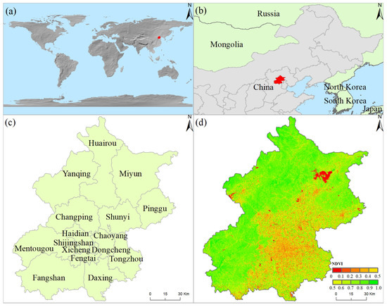
Figure 1.
Spatial map of the geographic study area. (a) Location of the Beijing (red colour) worldwide, (b) Location of the Beijing (red colour) in Northern China, (c) Administrative division of the Beijing, and (d) Vegetation covers synthesized according to the maximum of normalized difference vegetation index from time series of environmental images in the year of 2021.
From the perspective of natural environments, Beijing has a warm-temperate, semi-humid and semi-arid monsoon climate, featuring a hot and rainy in summer, a cold and dry in winter, and a shorter spring and autumn. The annual frost-free period is 180~200 days and annual average sunshine hours are between 2000 and 2800 h. Beijing’s natural rivers flow through five major water systems (i.e., Juma river, Yongding river, Beiyun river, Chaobai river, and Ji canal river) with the meandering direction from the mountains in the northwest to the southeast. Most of these rivers flow through the plain area and finally merge into the Bohai Sea in Haihe river. The terrain of Beijing is characterised as high in the northwest and low in the southeast, with an average altitude of 43.5-m. In terms of mountains, the western part of Beijing is the west mountain, belonging to the Taihang mountains; Jundu mountain is in the north and northeast, belonging to Yanshan mountains. The Dongling mountain has the highest peak, and is located in the Mentougou district, West Beijing, with an altitude of 2303-m; the lowest ground level is in the southeast boundary of Tongzhou district. The zonal vegetation types in Beijing are mainly warm temperate deciduous broad-leaved forest and warm coniferous forest. Most plain areas are covered by farmland and towns. The vegetation types of low mountains are Quercus variabilis forest, Oak forest, Pinus Tabulaeformis forest, and Platycladus orientalis, the middle mountains are dominated by liaodong oak forest and the high mountains consist of birch trees and mountain miscellaneous grass meadows.
2.2. Workflow
To summarize the main process of this study, we provided the workflow of the study area (Figure 2). In this figure, we present the workflow for urban land development boundary production, the classification of urban land-use structures, and the component mapping of intra-urban lands, together. Additionally, the relationship between the hierarchical urban land mapping and the natural physical medium environments are also shown.
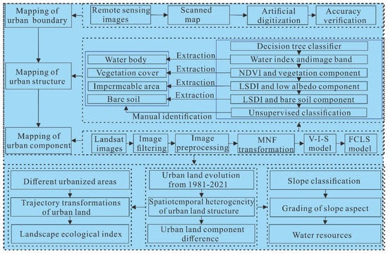
Figure 2.
The workflow of the study area.
2.3. Data Collection and Preprocessing
Data collection in this study mainly included two aspects, namely, the remote sensing data and the basic geographic data. Remote sensing was performed using Landsat MSS/TM/OLI, high-resolution Google images, and the digital elevation model. The images were mainly used to obtain the development boundary of urban land and its internal land structure as well as land components; and the digital elevation model performed spatial operation on ArcGIS platform to generate the physical medium environments such as slope and aspect. Basic geographic data include administrative divisions, road-loop network, national land-use data (NLUD), and water-resource distribution. Among them, NLUD provided the original boundary for urban land that needs to be revised. A spatial map of water resources was applied to analyze the relationship between urban land components and water resource service radius. All data were preprocessed using the unified coordinates and projections to ensure the accuracy of spatial mapping and statistical analysis. Descriptions of the collected data are provided in the Table 1 below.

Table 1.
The description of the main data that used in this study.
2.4. Establishment of Hierarchical Urban Land Mappings
2.4.1. Urban Land Development Boundary Production
In this study, to identify the entirely urban land boundaries, we referred to the land-use classification system of Resource and Environmental Science and Data Center, Institute of Geographical Sciences and resources, Chinese Academy of Sciences (website: https://www.resdc.cn) (accessed on 12 March 2021). The land-use classification system in this dataset has been widely used in national, regional, and local land-use change research in China. In this classification system, urban land (i.e., the land use type was coded as 51) was defined as land with a combination of high, medium, and low-density built-up areas. The benefit of this definition was to support a more comprehensive range of urban land by considering the urban and town areas [40,41]. In the context of this definition, urban land was defined as the same type of underlying surface of the urban and town areas, which can provide a uniform and spatially continuous land surface, avoiding the hollow and discontinuous regions within the urban and town boundaries.
For the urban land boundaries in 1981, 1991, 2001, 2011, and 2021, we extracted the urban land (shape file format) of the study area in 1980, 1990, 2000, 2010, and 2020 from the National Land Use Data of China, Institute of Geographical Sciences and Resources, Chinese Academy of Sciences. For the city boundaries of 1981 and 1991, Google historical archive images were first considered, but there was a large number of discontinuous boundaries in the study area. The number available Google images in the years of 1981 and 1991 in the study area was too little to carry out urban boundary studies in our investigation. Considering the difficulty of obtaining high spatial resolution and continuous coverage images for the whole study area before 2000, land resources satellites (i.e., Landsat images) from the years of 1981 and 1991 were used. We filtered the images of poor quality with issues such as cloud cover and bad pixels to obtain effective observations in summer (mainly July and August). All the downloaded images were synthesized by false color and displayed on the ArcGIS platform. We superimposed the vector city boundaries on the corresponding Landsat image. Human computer interaction digital technology was used to modify urban land boundaries by identifying the urban land texture, color, patches, and other features through professionally geographical knowledge. In the process of digitization, we controlled the polygon error within two pixels and obtained the urban-land boundaries in 1981 and 1991. Then, to reduce the inconsistency of urban boundaries caused by the use of Landsat image (i.e., 1981 and 1991) and Google image (i.e., 2001, 2011, and 2021), the early urban hand drawn map in the study area was digitally scanned and used as a reference to correct the urban boundaries. Although the scanned map had the problem of spatial geometric correction, it provided an essential reference for urban boundaries in the difficulty of obtaining sufficiently high spatial resolution images. As a result, the urban land boundaries were further modified to improve the accuracy of the boundaries in the years of 1981 and 1991. For the urban land boundaries after 2000 (i.e., 2001, 2011, and 2021), we obtained the 2 m resolution provided in Google’s historical archives by the authorized 91 bitmap platform, as high spatial-resolution remote sensing images have been effective since 2000. Similarly, using the high-resolution Google data for the natural background image, we obtained the urban land boundaries in 2001, 2011, and 2021 by modifying the urban land boundaries with manual digitization technology. Additionally, the administrative-division materials of the study area were also used as a reference in consideration of the administrative division change factors in the past four decades. Then, we obtained the required urban land boundaries for the years of 1981, 1991, 2001, 2011, and 2021, respectively.
2.4.2. Component Mapping of Intra-Urban Lands
A collaborative methodology of “satellite images—vegetation impervious surface area soil model—endmember decomposition model—multiple index—decision tree classifier—unsupervised classification—spatial analysis” was created to obtain the land use structure and its component data for the urban land in this study. Specifically, all the Landsat images for the summer of 1981, 1991, 2001, 2011, and 2021 were evaluated and obtained in the weather conditions of sunny and windless. The method of radiometric calibration was firstly applied to these images on the Environment for Visualizing Images Platform (ENVI). The fast line-of-sight atmospheric analysis spectral hypercubes (FLAASH, [42]) were used for atmospheric correction for the images obtained for the years of 1981, 1991, 2001 and 2011, so as to standardize the spectrum of each land type in urban areas. Furthermore, the Landsat OLI images acquired in 2021 were atmospherically corrected by a land surface reflectance code (LaSRc) algorithm from USGS earth resources observation and science (EROS) data center. After that, minimum noise fraction rotation (MNF Rotation) concentrated these land surface spectra in the first-three spectral features (generally higher than 90%). A visual interpretation of the MNF-based pairwise scattergrams from the first-three features was performed to obtain pure spectral endmembers to solve the vegetation–impervious surface area using the soil model (V-I-S, [23,43]), which was critical and directly affected the accuracy of the urban-land classification structure and its component products. In this process, a combination of automatic model extraction and manual recognition was used to filter pure endmembers. We obtained several sets of pure endmembers for each land class, which was input in the fully constrained least-squares solution model (FCLS, [44]) to generate the component images of the vegetation object, soil object, low albedo object, and high albedo object from Landsat images in the years of 1981, 1991, 2001, 2011, and 2021, respectively. Spatial analysis operation was used to produce the component image of impervious surface area. To further obtain better results, we filtered these density maps through field investigation data and a digitization of the land types of impervious surface area, vegetation cover, and bare soil using historical high spatial resolution images from the years of 2001, 2011, and 2021. Furthermore, we used a combination of Landsat images and the early urban hand drawn map from the years of 1981 and 1991, respectively, to eliminate the interference of the mixed pixel spectrum issues. If the error of the decomposition result was high, we continued to optimize the endmembers until a better density map was obtained. Then, the density maps of impervious surface area, vegetation cover, and bare soil with the sub-pixel values of 0.01~100.00% were obtained for the years of 1981, 1991, 2001, 2011, and 2021, respectively.
2.4.3. Classification of Urban Land Use Structure
Spectral features were often used for urban land classification; however, the issue of mixed pixels at the pixel level led to interference in the classification accuracy. Generally, bright high albedo objects were disturbed by bare soil, while low albedo objects were disturbed by building shadows and water bodies. To weaken the interference of these factors, in this study, we obtained urban classification products by the process of “pixel—sub-pixel—pixel”. Firstly, for the pixel level, we downloaded all Landsat images that needed to be classified in the study area from the USGS official website. We performed image preprocessing on these images at the pixel level. Secondly, the process for images from pixel to sub-pixel levels was performed. The main processes of MNF transformation, endmember selection, vegetation—impervious surface area—soil model and fully constrained least-squares solution model were applied to obtain the sub-pixel images of impervious surface area, vegetation cover, and bare soil, with the sub-pixel values of 0.01~100.00%, respectively. A detailed description of sub-pixel extraction is provided in Section 2.4.2. Finally, the process of sub-pixel to pixel levels was undertaken. In this process, the interference of mixed pixels was reduced at the sub-pixel scale, to obtain more accurate classification results. In this study, we carried out the sub-pixel to pixel process through the combination of a decision-tree classifier and manual observation. The process is detailed below. The modified normalized difference water index (MNDWI, [45]) was firstly used to extract water bodies through the combination of green and NIR from Landsat images, which was applied to mask the interference signal from dark high albedo objects. Then, the synergism of the vegetation cover component data and the normalized difference vegetation index (NDVI, [46]) was used to extract vegetation types. The low-albedo and soil difference index (LSDI) proved to be an effective method to eliminate the spectral interference of bare soil in the bright high albedo objects. The combination of LSDI and soil component data was used for the extraction of bare soil. After that, the low and high albedo objects were applied to obtain the cover of impervious surface area. Then, the remaining unclassified surface types (usually less than 5%), were addressed through unsupervised classification. In this study, the unsupervised classification divided the unclassified region into 50 types (i.e., the 50 images) in each Landsat image. The manual observation of the spatial position as well as the optical characteristics from each unsupervised classified image were used to identify the land use types. Finally, all the classified land types were integrated into four categories, including the impervious surface area, vegetation cover, bare soil, and water body in the urban land regions.
2.5. Selection of Urban Land Landscape Index
The landscape index has always been applied to describe the spatial organization form and spatial allocation information of land use structure, acting as an effective way to explore the fragmentation, advantages, connectivity, aggregation, mosaic, and diversity of land surface [47]. Generally, a single index was not adequate to express these characteristics of land types, but too many indexes would become repetitive and redundant. We selected as few indexes as possible to express the required characteristics, referring to the guidance manual of landscape meaning. Finally, the patch density, aggregation index, connectivity index, largest patch index, landscape shape index, and Shannon’s diversity index were obtained from the two scales of landscape type level and landscape diversity level to explore these characteristics [48]. The name, abbreviation, formula, and definition of all landscape indexes are provided in the following table (Table 2).
Table 2.
The name, formula, and definition of the selected landscape index in this study.
2.6. Division of Physical Medium Environments
In this study, we focused on the physical medium environments of slope, aspect, and water resource service, because these natural conditions were considered significant and may intuitively overlap with the urban land component data using the spatial clustering analysis, to form a geographical map of spatial visualization. It provided the advantage, in this study, of exploring the issue at the sub-pixel scale, namely, the relationship between sub-pixel urban land component and the physical medium environments (slope, aspect, and river distribution) was investigated, to provide a new evaluation.
The fluctuation of slope often affected the spatial distribution of buildings, which was an indispensable factor that must be considered in the building construction. To obtain the variable of slope, a spatial analysis module from ArcGIS was opened first, following which we navigated the surface analysis tools. Inside the surface analysis group, the slope analysis tool appeared and was applied to identify the slope (gradient or steepness) from each cell of a raster using the input of digital elevation model (DEM), for generating the spatial slope map. To facilitate the spatial analysis of slope and urban land component data, the classification tool was applied to divide the slope map variable into five levels, with values of [0~5°), [5°~10°), [10°~15°), [15°~22.5°), and (>22.5] from level 1 to level 5, according to the harmfulness reference of the slope to buildings, etc. Similarly, the building density in each pixel of the aspect always reflected the orientation of the building. During the preprocessing of aspect data, the aspect variable was divided into eight directions at an interval of 45 degrees clockwise through a similar method to that used to produce the slope map. The direction of aspect map included the North [0–22.5°), Northeast [22.5°–67.5°), East [67.5°–112.5°), Southeast [112.5°–157.5°), South [157.5°–202.5°), Southwest [202.5°–247.5°), West [247.5°–292.5°), Northwest [292.5°–337.5°), and North [337.5°–360°), respectively.
Water resources within the city such as the rivers, lakes, and ponds played a considerable role in regulating the hydrological process of the urban ecosystem and the comfort of human settlements. The evaporation from the water body was conducive to increased air humidity and reduced local polar heat. The distance from the river became an important index to measure this regulation of water resources to urban residential and living areas. The service radius of water resources was set as 0.5 km, 0.5–1 km, and 1–2 km according to the survey of the buildings, roads, and squares in the study area. This buffer service radius not only ensured that the patches did not overlap as much as possible, but also ensured the full coverage of impervious surface area components. Additionally, although the road was considered to be a result of planning, we still explored the distribution characteristics and spatiotemporal evolution law of urban land and its structure in different loops (mainly the typical loops from 1 to 5), considering the urban land development characteristics of the loop line in the past 40 years in the study area.
2.7. Accuracy Evaluation Scheme
Urban land mappings in this study were created according to spatial expansion dimension, the internal land structure change dimension as well as its component dimension, displaying a hierarchical urban land classification system. For the land expansion, urban land boundaries were based on the coordination of 2 m Google images, historical city maps, and high spatial resolution land products. Thus, we focused on the accuracy evaluation of the urban structure and its components. For the land use structure, facing the dilemma of validation in 1981 and 1991 due to the difficulty in obtaining the high resolution image, we designed a cross validation scheme from Landsat images, namely, the verified Landsat images were separated from the images used to obtain a time series of land-use structures and the land use components in the study area, i.e., we used some images to obtain land use structures and their components; furthermore, we employed other images in the same year to conduct accuracy verification. After that, a stratified random sampling technique was applied to generate a total of 7500 sampling points, following which the Landsat images for the years of 1981 and 1991 from the USGS website and the 2 m Google image in the years of 2001, 2011, and 2021 from the authorized and professional 91 bitmap platform were obtained. Taking these images as the background data, we superimposed all the samples to the imagery and manually checked the samples one by one to identify the true and false values. An accuracy evaluation matrix was used for accuracy calculation, along with the indicators of classified samples, reference samples, the number of correct samples, ground truth samples, producer’s and user’s accuracy, using the verified samples. For the land-use component validation, a 3 × 3 pixels window (pixel) method was applied to calculate the actual land surface area, with a total number of 100 in each land type. To facilitate the verification, we divided each land component data into 10 levels, with a 10% component interval from level 1 to level 10. Then, we compared the actual values with the reference values (i.e., the land component generated in this study) to calculate using the combination of fitting coefficient (R2) and mean square error (RMSE).
3. Results
3.1. Accuracy Evaluation Results
The verification of two scales, including the urban land structure at the pixel scale and its components at the sub-pixel scale, was performed. For the land structure scale, a total of 7500 samples (i.e., 1500 samples at each year) were applied and randomly overlayed on remote sensing images, to obtain the ground truth pixels of impervious surface area, vegetation cover, bare soil, and water body (Table 3). An accuracy evaluation matrix was then formed to show the correct and wrong number of samples. Indicators of user’s accuracy, producer’s accuracy, number of correct samples, reference pixels, and classified pixels were calculated. We obtained the number of correct samples of 1387, 1393, 1360, 1371, and 1394 in the years of 1981, 1991, 2001, 2011, and 2021, with the comprehensive evaluation accuracy of 92.46%, 92.86%, 90.67%, 91.40%, 92.93%, and kappa coefficient of over 0.85 for the study area, respectively. The data show that we obtained a better accuracy in each studied year. For the land component scale, the method of land-component data classification, with a 10% component interval from level 1 to level 10 (i.e., the component value from 0.01% to 100%), was applied to improve the accuracy evaluation. A combination of actual values and reference values was used to calculate the accuracy. Additionally, we obtained the fitting coefficient (R2) and mean square error (RMSE) over 0.8965 and 12% in each studied year.
Table 3.
Accuracy evaluation matrix and indicators in years of 1981, 1991, 2001, 2011, and 2021.
3.2. Spatial Evolutions of Urban Lands in the Whole Study Area and in Regional Differences during 1981–2021
In the whole study area, the rate of urban land occupation (i.e., the rate of urban land to the administrative area of Beijing) was only 2.85% in the first studied year. Then, an intense and sustained urban land expansion was identified, which resulted in the corresponding proportional value reaching 15.73% by the end of the studied period (Figure 3). This implies that urban-land occupancy has increased by 5.53 times in the past 40 years in the study area. For the urban land itself, total urban land covered the area of 467.13 km2 in the year of 1981. The coverage increased by by 141.14 km2, 625.29 km2, 962.24 km2, and 385.25 km2 during the ten-year intervals during the studied period. As the dynamic change data showed, the urban land increments in each interval of the study area did not display an accelerated expansion. In fact, the average annual urban land expansion accelerated from 1981 to 2011, and then slowed down from 2011 to 2021. Finally, total urban land area reached 608.28 km2, 1233.56 km2, 2195.80 km2, and 2581.05 km2 in the years of 1991, 2001, 2011, and 2021, respectively, with a total urban land increment of 2113.93 km2 during 1981–2021. For the changes in the spatial distribution of urban land, the urban built-up area expanded in all directions at the beginning period and then focused on the directions of north, northwest and southwest, as the eastern region of the study area was close to the edge of administrative boundaries, and urban land expansion in this direction was limited.
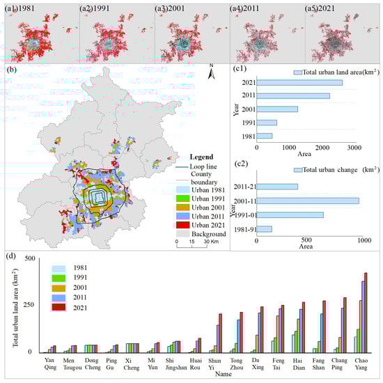
Figure 3.
Spatial evolution of urban land in the whole study area and its regional differences from 1981 to 2021. False color synthetic Landsat images in the years of (a1) 1981, (a2) 1991, (a3) 2001, (a4) 2011, and (a5) 2021, with the R, G, B bands of 6, 5, 4 from MSS, the bands of 4, 3, 2 from TM5, and the bands of 5, 4, 3 from OLI8; (b) Spatial evolution pattern of urban land expansion from 1981 to 2021 in the whole study area; (c1) Statistics of total urban land area in the years of 1981, 1991, 2001, 2011, and 2021, respectively; (c2) Statistics of urban land area change in the periods of 1981–1991, 1991–2001, 2001–2011, and 2011–2021, respectively. (d) Total urban land and its change at the district level from 1981 to 2021, including the regions of Yanqing, Mentougou, Dongcheng, Pinggu, Xicheng, Miyun, Shijingshan, Huairou, Shunyi, Tongzhou, Daxing, Fengtai, Haidian, Fangshan, Changping, and Chaoyang, respectively.
In different regions, urban-land expansion displayed obvious differences in the quantitative changes and spatial distribution patterns. In the initial year, the urban land occupation rate changed from 0.11% (i.e., Yanqing) to 99.93% (i.e., Xicheng), indicating a huge difference (Table 4). Only six districts were over 18.00% and other regions were all lower than 3.00%. At the end of the studied period, the corresponding value was increased by more than 18.00% in ten districts, and only three districts were lower than 3.00%. The districts that contained built-up areas had a high urban occupancy rate (i.e., the rate was already 100% in Dongcheng and Xicheng in the year of 1991). On the contrary, a low rate was consistent for the districts far away from built-up areas such as Yanqing (2.49%) and Miyun (1.94%) in 2021. Meanwhile, in the past 40 years, all regions have experienced the process of urban land expansion, with the largest increment in Chaoyang (i.e., +334.97 km2) and the smallest increment in Xicheng (i.e., +0.03 km2). From the perspective of a spatial pattern, urban land was mainly concentrated in the districts of Xicheng, Dongcheng, Shijingshan, and Haidian in 1981. Then, urban land intensely moved towards the regions of Chaoyang, Fengtai, Tongzhou, Daxing, Changping, and Shunyi during the period of 1981–2021. Currently, there are still four districts, including Yanqing, Huairou, Miyun, and Pinggu, that are not spatially linked to the built-up areas, and thus the evolution of urban land was relatively slow in these regions over the studied period.
Table 4.
The statistics of urban land occupation rate at the district level in different time stages from 1981 to 2021 in the study area (Area unit: km2, Rate unit: %).
3.3. Evolutions of Urban Land Use Structure in the Study Area and Their Trajectory Transformations in Different Urbanized Regions
3.3.1. Urban Land Use Structure Evolution at the Study Area and at the Land Type Scales
The land use structure within the city was divided into four types in this study, including impervious surface area (ISA), vegetation cover (VC), water body (WB), and bare soil (BS), all of which experienced different evolutionary processes in the past four decades. At the level of the whole city, the proportion of ISA, in terms of the whole city, accounted for half (53.67%) of the built-up area in the initial year (Figure 4). Then, a continuously incremental cover rate of ISA was observed, with 66.21%, 69.37%, 71.82% and 73.62%, in the years of 1991, 2001, 2011, and 2021, respectively. This indicated that ISA increased by 19.96% under the fast urbanization process throughout the study period. On the contrary, the proportion of VC to the whole city continuously reduced with a cover of 43.70% in the initial year and 24.80% in the final year, with a total reduction of 18.89%. Meanwhile, the proportion of WB and BS to the whole city displayed a slightly downward trend with a change of 0.32% and 0.74%, respectively. Overall, the proportion of land use in cities was characterized by the increase in ISA and the decrease in VC, as well as the relative balance of WB and BS in the urbanization process throughout the study area over the past 40 years.
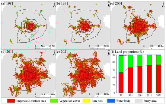
Figure 4.
Spatial land structure changes and their statistics in Beijing from 1981 to 2021. Note: (a–e) represented the spatial structure of land use in Beijing in the years of 1981, 1991, 2001, 2011, and 2021, respectively; and (f) represented the statistics of land use changes during 1981–2021.
For the area cover of land types, all land use types have experienced different degrees of expansion during 1981–2021. The most dramatic extension occurred in terms of ISA compared to other land types, covering an area of 250.69 km2, 402.77 km2, 855.71 km2, 1577.06 km2, and1900.23 km2 in the years 1981, 1991, 2001, 2011, and 2021. Total cover of ISA increased by 1649.54 km2 throughout the study period, indicating a sharp growth rate of over 650.00%. Considering that Beijing is China’s political, economic, cultural, transportation, and talent center, the drastic ISA expansion not only met the needs of urban infrastructure construction, but also for peoples’ living, working, and leisure facilities, which led to the divergent spatial patterns of ISA expansion in all directions, with the spatial evolution dominated by concentration and contiguity. In addition to the ISA, the cover of VC has also shown rapid growth in the past 40 years with the areas of 204.12 km2 in 1981 and 640.22 km2 in 2021, a total growth rate of 213.64%. Newly expanded vegetation was mainly used for the greening urban residential areas, roads, squares, and parks during the urbanization process to regulate the urban microclimate. Specifically, most of the VC was scattered in the central area of the city, and there were a large number of concentrated contiguous regions not far from the urban fringe. The number of water bodies, mainly in the forms of ponds and slender rivers, also acted as an important indicator of urban climate regulation, with a change of +4.37 km2 during 1981–2021. Although the study area was located in the humid climate region, a small increase in bare soil expansion was still detected with area coverage increasing from 9.51 km2 to 33.43 km2, mainly located at the sites being constructed.
3.3.2. Trajectory Transformations of Urban Land Use in Different Urbanized Regions
The transformation trajectory of urban land use can provide a mechanistic explanation for land-use change in urban regions, which usually acts as an indispensable aspect of urban-structure analysis. In this study, the differences of urban land structure in different urbanized regions (i.e., the old urban regions (OUR) and the newly expanded urban regions (NEUR)) were tracked (Table 5). During the period of 1981–2021 in the OUR, 96.68% of the original ISA region was preserved; and only 3.32% shifted to other land types, i.e., 2.91% for VC, 0.01% for WB, and 0.40% for BS. The area of newly expanded ISA in OUR was 179.38 km2; and the contribution rate of other land types to new ISA in OUR was 95.30% from VC, 1.32% from WB, and 3.38% from BS, respectively. Therefore, a large amount of new ISA and a small decrease in ISA increased its net increment of 171.06 km2, indicating a more compact living environment space in OUR in 2021 compared to that of 1981. Although vegetation loss was found to be high in the OUR, the proportion of vegetation cover to urban land remained at 8.43%, which means that vegetation can still play a significant role in regulating the urban living environment in OUR considering appropriate vegetation cover.
Table 5.
Urban land trajectory transformations in different urbanized regions (Area unit: km2).
For the newly expanded urban region (NEUR), the cover of the original ISA was 105.58 km2, which accounted for 90.58% of the total ISA in this region by 1981. Although this land use is still characterised as ISA, its function changed from rural land to urban land, such as urban residential areas, roads, squares, etc., during the urbanization process of 1981–2021. The loss of ISA was small, with a total area loss of only 10.98 km2, which may be mainly used for green space planning in the process of land function transformation from rural to urban. Meanwhile, a high expansion of ISA was observed in the NEUR, with a total area of 1392.90 km2. The data demonstrate that the newly expanded ISA in NEUR was 7.65 times than that of OUR in the same period. In the NEUR, 97.73% of the newly expanded ISA was from previous vegetation area, as the study area was located in a humid region and mainly surrounded by a vegetation green system. The total contribution rate of WB and BS to new ISA was only 2.27%. Against the background of a humid climate, 97.97% of the vegetation loss was converted into new ISA. However, the proportion of vegetation cover to the urban land remained at 28.42%. This implies that vegetation can play a useful role in ecosystem services in the NEUR considering the high vegetation cover. This value was much higher than that of OUR (28.42% in NEUR vs., 8.43% in OUR).
3.4. Spatial Configuration Characteristics of Landscape under the Background of Land Structure Evolution in the Study Area during 1981–2021
At the landscape level, the urban landscape of the study area during the period of 1981–2021 changed significantly due to the drastic land-use change within the city (see Figure 5). There was no doubt that the number of land patches increased rapidly in the process of urbanization, with total patches increasing from 11,346 to 42,495, at a growth rate of 274.54%. However, the degree of landscape fragmentation throughout the city reduced with the PD change of −8.305. In other words, the integrity of urban landscape (SHDI= −0.164) has been enhanced over the past 40 years. On one hand, the dominance of landscapes continued to increase as the LPI changed from 35.295 to 59.590, as well as the landscape aggregation (AI= +4.621). On the other hand, the evolution of different land-surface types weakened the horizontal landscape linkage (CON= −0.265) at the per-unit-distance scale considering the complexity of landscape reorganization.
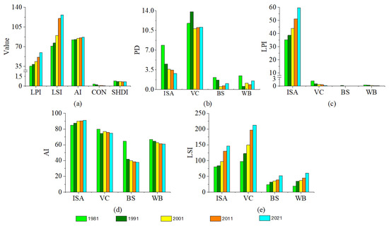
Figure 5.
Ecological landscape change in the study area during the period of 1981–2021. Note: (a) represented the index change of landscape scale; and (b–e) represented the index change of type scale for PD, LPI, AI, and LSI, respectively.
At the different land-use type level, the continuous cluster and expansion of impervious surface areas meant landscape aggregation continuously improved, with AI values of 84.93, 87.60, 88.37, 90.10, and 91.11 in the years of 1981, 1991, 2001, 2011, and 2021, respectively. Correspondingly, the landscape advantages of the ISA also increased in each studied period, with 35.29 in the initial year and 59.59 in the last year. These changes promoted the continuity of the ISA per unit area and decreased its fragmentation (PD= −5.02). On the contrary, the uninterrupted cutting of ISA expansion to vegetation cover and bare soil led to both land types becoming more broken over the studied period, although there were lots of large-scale green parks in urban-land regions. Additionally, the advantages of both land types followed the decreasing trend, with LPI changes of −3.34 and −0.02 during 1981−2021, respectively. A common change feature for all land types was that the LSI increased by varying degrees for different land use, with changes of 49.69, 115.36, 18.54, 25.68 for ISA, VC, BS, and WB from 1981 to 2021, respectively.
3.5. Analysis of Urban Land Component Characteristics on a Spatiotemporal Scale
The component changes of different land-use types within the context of urban land can help to elucidate the advantages of the lands’ temporal and spatial heterogeneity at a sub-pixel scale. In this study, the component maps of impervious surface area, vegetation cover, and bare soil, with component values ranging from 0.01 to 1.00 during 1981–2021 have been presented and analyzed (Figure 6). For the urban land boundary of 1981 (i.e., the old urban land region of 2021 (OULR2021)), we evaluated that the average component of ISA was 0.659, which was lower than that of 0.739 in the OULR2021, indicating a component increment of 0.080 in the old urban region. This increment not only means the expansion of ISA on the sub-pixel scale, but also includes the cover changes of buildings, squares, roads, etc., in the unchanged ISA region, considering that this study only displayed two-dimensional ISA maps. At the same time, the opposite trend to ISA occurred for vegetation cover and bare soil, with average component changes of −0.404 and −0.198 in this region, respectively. The data display that a higher density loss occurred in vegetation cover compared with bare soil throughout the studied period.
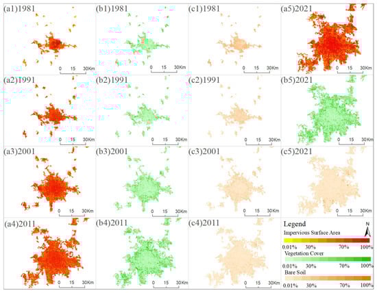
Figure 6.
Urban land component in types of impervious surface area (red), vegetation cover (green), and bare soil (yellow) with values from 0.01% to 100% during the period of 1981–2021, respectively. Note: (a1–a5,b1–b5,c1–c5) represented the land component types of impervious surface area, vegetation cover, and bare soil in each year, respectively.
Compared with the OULR2021, in the new urban land region of 2021 (NULR2021, i.e., the urban land expansion region during 1981–2021)), we found that the average component of ISA was 0.615, which was much lower (−0.178) than the corresponding value of ISA in the OULR2021. The concept of low-density ISA construction may be applied to the urban expansion of the study region. On the contrary, a higher average density of vegetation cover was observed in NULR2021 compared with that of OULR2021 (i.e., 0.304 vs. 0.193), implying that a new green urban region may have been formed. Meanwhile, the average component of bare soil in NULR2021 was a little higher than that for OULR2021 due to more sites being constructed. On the whole, we detected a lower average component of ISA (0.637 vs. 0.659) and BS (0.079 vs. 0.030) and a higher average component of VC (0.284 vs. 0.211) in the urban land boundaries of 1981 and 2021 using comprehensive statistics for the studied period.
3.6. The Relationships of Multiscale Land Use Distributions with the Physical Medium Conditions
3.6.1. Urban Land and Its Land Use Structural Evolution in the Traffic Loops during 1981–2021
The roads in the study area were mainly characterized by loop lines, from loop line 1 (L1) to loop line 5 (i.e., L2, L3, L4, and L5, separately). The traffic loops evidently affected the change of urban land and its cover structure during the past 40 years, which is explored in this section. During the urbanization process, the L1 was located in the centre of the urban area (i.e., the innermost loop) and covered the full urban area by 1991 (Table 6). Similarly, this was observed for the L2 and L3 in the same year of 2001; but the same did not occur for L4 and L5 over the study period, with a ratio of urban land to corresponding loop area of 99.99% and 68.73% in the year 2021, respectively. Therefore, the future urban land development of the study area will focus on the 5th loop or even on the wider regions. Meanwhile, the total cover of ISA increased from 232.35 km2 in 1981 to 1358.27 km2 in 2021 within the loop lines, with an increment of 4.85 times; and then, the ratio of ISA to the corresponding loop region in 2021 amounted to 92.05%, 92.72%, 90.33%, 78.50%, and 49.64% from L1 to L5, respectively. The data showed that the ISA was mainly distributed within the third loop line. On the contrary, the ratio of VC to the corresponding loop region in 2021 was low in the central urban region and high in the urban fringe region, with rate of 5.29%, 6.16%, 8.98%, 20.19%, and 17.77% from L1 to L5, indicating that the highest rate appeared in the fourth loop line (L4). Similarly, only 6.41% of the water body was distributed in L1, but 68.72% were located in L5, indicating the existence of a low proportion of water bodies in the central urban region and the high proportion of water bodies in urban fringe region. We also observed that the cover of bare soil almost disappeared from L1 to L4, with a cover area of only 3.33 km2 in L5. Overall, urban land and its cover structure have obviously changed within different loop line regions in the past 40 years of the study area.
Table 6.
Urban land and its structural covers within each loop lines in the study area during the period of 1981–2021 (Area unit: km2).
3.6.2. Analysis of the Distribution of Land Use Components with Slope and Aspect
Although the study area was located on the North China Plain with flat terrain, it still had large local undulation, with slope gradation areas of 1643.43 km2, 764.55 km2, 127.23 km2, 31.08 km2, and 6.87 km2 from level 1 to level 5 in the whole study, respectively. Thus, most (i.e., over 92.00%) of the impervious surface area and vegetation cover were distributed in the flat area due to the topographic background, but the difference between the two was still captured. The proportion of high- and medium-density vegetation cover was greater than that of the impervious surface area (i.e., 1.74 vs. 1.58 and 1.65 vs. 1.44), considering that the high slope was not suitable for building construction such as Level 4 and 5. We also investigated the distribution of impervious surface in areas with higher slopes, and found it was mainly distributed in expressway areas and tourist attractions such as Xiangshan and Qinglongxia parks, which did not serve mainly residential needs. The study provided a quantitative evaluation of impervious surface area distribution, with a distribution rate of 64.17%, 29.45%, 4.90%, 1.21%, and 0.27% from the slope level 1 to level 5, respectively.
From the perspective of impervious surface area distribution and aspect, the dominant aspect (i.e., South) was observed, with the cover areas of 63.98 km2, 244.81 km2, and 106.00 km2 from the low-, medium-, and high-density ISA. These areas accounted for 16.05%, 16.11%, and 16.18% of the total area of the corresponding density region, respectively. The second advantage was North, with the corresponding density areas of 59.85 km2, 232.71 km2, and 101.83 km2. Perhaps the North–South impermeable design was more in line with the orientation of buildings in the study area; and thus, the North–South slope was more popular with impervious surface area than other directions (i.e., Northeast, East, Northwest, West, Southwest, and Southeast). The direction of minimum ISA distribution (i.e., West) was also captured, with a cover of 36.81 km2, 147.23 km2, and 65.77 km2 from the low-, medium-, and high-density regions, respectively.
3.6.3. Analysis of the Relationship between Land Use Components and Water Resource
The relationship between land use components and the water bodies can describe the hydrological services of the inner city to some extent. To distinguish this relationship, we counted the characteristics of impervious surface area and vegetation cover components with water bodies using the service radius of 0.5 km, 0.5–1 km, and 1–2 km away from the water (i.e., rivers, reservoirs, lakes, and ponds, Figure 7). Within a 0.5 km water resource service radius, the proportion of high-, medium-, and low-density ISA to the buffer zone was 23.67%, 61.28%, and 15.06, indicating that medium-density ISA was dominant. The surrounding areas of these waters were basically tourist attraction according to our field survey; and a reasonable distribution of ISA and VC was conducive to relax the mind and spirit of tourists. However, the value of high density ISA was still very high in some regions within a 0.5 km water resource service radius. The roads, squares, food, and residential areas and other ISA usually formed an accumulation of high-density ISA areas, such as the surrounding area of Shichahai, a tourist attraction in the study area. The cover of low-density ISA was very low and was mainly distributed in the concentrated area of vegetation cover, such as the botanical garden and forest park. Additionally, the proportion of high-, medium-, and low-density of VC to the buffer zone was 28.66%, 43.75%, and 27.58%. High-density VC was higher than ISA in the buffer zone.
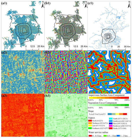
Figure 7.
Spatial diagram of urban land components and physical medium environments. (a1,b1,c1) represent the spatial distribution of slope, aspect, and water resources. (a2,a3,b2,b3) represent a same sample region of the slope, aspect, impervious surface area component, and vegetation cover component; and (c2) represent a sample region of water resources service radius, respectively.
When the water-resource service distance changed from 0.5 km to 0.5–1 km, and 1–2 km, the cover rate of high density ISA showed an increasing trend, with values of 23.67%, 26.46%, and 32.21%. On the contrary, high-density VC displayed a decreasing trend, with 28.66%, 17.63%, and 9.67%, respectively. The data showed that high-density ISA was relatively low but high-density vegetation was relatively high in the buffer zone closest to water resources. The low-density ISA was relatively stable, at around 15%, within each service radius; but the low-density VC increased from 27.58% to 52.31%, with a total increment of 89.66%, indicating that low-density VC was usually distributed in the regions far away from water resources. A common land use feature was observed, with the medium-density ISA and VC in the dominant types in any water resource service radius areas, reflecting that the urban land in the study area emphasized the mosaic distribution pattern of ISA and VC.
4. Discussion
4.1. New Reports on Multi-Scale Urban Land Evolution in Capital City of China during 1981–2021
Our study first revealed the new multi-scale urban land change (i.e., land use, land structure, and land component) during 1981–2021 according to the remote sensing methodology, to describe the spatiotemporal heterogeneity of the urban surface. Specifically, a total urban land expansion of 452.53% was observed during 1981–2021, along with an annual expansion rate of 11.31%/yr. This annual growth rate was much higher than the corresponding value in China’s arid urban land areas (i.e., the 3.60%/yr during 2000–2014 [49]). Considering that the study area was China’s political, economic, and cultural center, it already ranked first in terms of urban expansion over the studied period of 2000–2015 within the Global Belt and Road (followed by Bangkok (Thailand) and Kuala Lumpur (Malaysia)) [26,50].This study extended the scope of urban expansion of the study area to the year of 2021, providing an updated reference for the comparison of capital urban-land expansion within the “belt and road”.
In addition to urban land boundary change, our classification of urban land structures mainly focused on two land use types, including the impervious surface area (ISA) and vegetation cover (VC). ISA included the roads, squares, building roofs, and other regions where rainwater cannot pass through. ISA often led to issues such as high land-surface temperature and non-point source pollution of rainwater on a local scale, affecting the well-being of urban human settlements. In this study, the ISA was also characterized people’s places of work and residence; and ISA was the most important land structure change in the study area along the past 40 years. With the migration of a large population and the improvement of urban infrastructure, a change in ISA occurred over time. Additionally, the VC, with urban expansion and impervious surface area change, also experienced change according to our study. The effects of nitrogen fixation, oxygen release, and water conservation from VC played a very important role in regulating urban residential environment, Thus, the framework/structure of ISA and VC change proved to be important for the study. We discuss the findings of VC and ISA in the following two paragraphs.
For the urban land structure change, a greening study area was observed with a vegetation coverage rate of 8.43% in the old urban regions (OUR) and 28.42% in the newly expanded urban regions (NEUR)), indicating that, in the process of urban expansion, more attention was paid to the construction of vegetation to improve the ecosystem service function of a green system [51,52]. Additionally, the expansion of an impervious surface area into green space often led to a cutting effect. This means that the complete green space was divided into many blocks, reducing the landscape dominance (i.e., LPI) and increasing the fragmentation (i.e., PD) of vegetation. Furthermore, the enhancement of spatial interaction between impervious surface area and vegetation may have increased the comfort of residential and living environments [53,54]. The concentrated vegetation appeared more in the surrounding areas of the urban land such as the fourth and the fifth ring roads in the study area, which may play a role in wind prevention and sand fixation around the urban land [55].
For the urban land component change, although the urban appearance of the study area has changed dramatically in the past 40 years, such as the transition from ordinary brick houses to high-rise buildings [56,57], the average composition of ISA only increased from 0.659 in 1981 to 0.739 in 2021 in the old urban land regions. The data showed the impervious surface coverage component in the study area was high in the initial year of the study. An increment of 0.080 in the old urban region on a two-dimensional scale during 1981–2021 included the expansion of ISA and changes to the form of ISA such as buildings, roads, and squares. Meanwhile, in the year of 2021, a lower (−0.178) average component of ISA and a higher (+0.111) vegetation cover was observed in the new urban land regions compared with that of old urban land regions. Low-density ISA and high-density vegetation construction have become the main features of urban expansion, considered to be conducive to the well-being of human settlements [58,59].
The mapping of the spatiotemporal patterns of the urban impervious surface can serve a few purposes. In this study, a multi-scale urban land mapping methodology was established using time series of Landsat imagery and a remote sensing technique to display the new spatiotemporal heterogeneity and the evolution of urban land, including indicators of urban land, land use structure, and its components in China’s capital city, Beijing, during the period of 1981–2021. In particular, the intra-component of urban impervious surface (UIS) can provide a density map at the sub-pixel scale. One of the advantages of a UIS density map is that it can show the percentage change in terms of the land surface energy when overlapped with the surface radiation energy balance index from the retrieved Landsat images, such as land surface temperature, latent heat flux, sensible heat flux, soil heat flux, and Bowen ratio [60]. The sub-pixel UIS that includes energy change can more accurately evaluate the thermal comfort of human settlements, which was found to have supported the planning layout of urban commercial or residential area construction in terms of the livable settings design for the urban planning department. Additionally, the sub-pixel UIS with an energy change in urban parks and scenic spots can be used to reasonably design a mosaic pattern of impervious surface area and green space, to reduce the extreme heat phenomenon in summer, for the local tourism department [61]. Furthermore, by using mapped spatiotemporal patterns of sub-pixel UIS with the topographic map, the emergency management department can evaluate the impact of geological disasters [62], such as landslide and debris flow on residential areas. Therefore, the sub-pixel UIS may have broad application prospects.
4.2. Findings of the Physical Medium Environments with Multi-Scale Urban Land Use Changes
Both low-, medium-, and high-density impervious surface areas were first distributed in the southern direction, followed by the northern direction. The north–south slope has become the dominant distribution direction of impervious surface area;, and we calculated the specific value of their distribution in the north–south slope of the study area. Considering that the study area was located in the northern hemisphere [63], and the natural succession law of the East rising and West setting of the sun, buildings facing north and south may be conducive to the sunlight entering the interior of the building for the increased brightness inside of the house [64]. Another factor was that north–south buildings are a traditional architecture feature of North China [65]. Of course, modern buildings also had east–west buildings according to the terrain. In ancient China, buildings facing east and west were called wing-room (Xiangfang) [65,66], especially quadrangles, and the owner mainly lived in the house facing north and south [67]. In addition, the north–south terrain was conducive to reducing the construction cost and became the advantageous living direction in North China.
For the slope in this study, over 92.00% of the impervious surface area and vegetation cover were distributed in the flat area due to the topographic background of the North China Plain. The constraints of terrain on urban expansion were minimal. However, the constraints of terrain on urban expansion were very strong in Southwest China due to the existence of a large number of mountains, which usually affected the spatial distribution and orientation of buildings [68]. In these areas, cities primarily expanded along valleys, such as Lanzhou, a provincial center city expanding along the East–West valley due to the mountains in the north–south [32]. For the water resource service and urban land structure component distribution, the cover rate of high-density vegetation displayed a decreasing trend, and the water resources service distance changed from 0.5 km to 0.5–1 km and 1–2 km. Vegetation was distributed closer to water resources. In contrast, high-density ISA showed an increasing trend along with the water resources service radius from the near to the far. Within a 0.5 km water-resource service radius, high-density impervious surface area was mainly distributed in tourist areas, such as scenic spot layout, roads, squares, catering, accommodation, etc. Residential areas and business centers are mainly distributed in the service radius of 0.5–1 km and 1–2 km according to the field survey. Water resources had a greater impact on the function of impervious surface areas, such as travel or residence [55,59].
4.3. Potential Cycle Effects of Urban Land Evolution on Carbon Peak/Neutralization
Climate change is a global problem faced by mankind [69]. With the emission of carbon dioxide and the sharp increase in greenhouse gases in various countries, it poses a threat to the ecosystem [70]. In this context, countries all over the world have aimed to reduce greenhouse gases by means of global agreements. Therefore, China puts forward the goals of “carbon peak” before 2030 [71], that is, carbon dioxide emissions will not increase and will then slowly decrease after reaching the peak; and “carbon neutralization” by 2060 [72], that is, carbon dioxide emissions will be offset by tree planting, energy conservation, and emission reduction. There is no doubt that carbon emissions in urban areas considerably impact the target of “carbon peak” before 2030 and “carbon neutralization” by 2060” [71]. It is promising that the characteristics of lower density impervious surface area and higher density vegetation were presented in the construction of the new urban land region compared with that of the old urban land regions in the study area, an epitome of China’s urbanization, which has been beneficial for absorbing more carbon dioxide to achieve carbon peaking and carbon neutralization goals [73].
Our study also found that the proportion of vegetation coverage in old and new urban areas was 8.43% and 28.42%, which showed that the city has turned green. This process is not accidental, but a microcosm of the greening of cities in the whole Eurasian continent since the year of 2000. This means that the global scale greening process is taking place within the region, thereby increasing the neutralization of carbon emissions worldwide [74]. Meanwhile, different land changes in humid and arid regions led to different carbon emission/sink, and land tracking technology in this study was applied to analyze the source and destination of interior-urban land type change [75,76]. We observed that the expansion of the impervious surface area occurred in areas of previous coverage cover (mainly croplands according to the field investigation) and bare soil (mainly from the construction sites and small feature regions). In this process, medium carbon density soil (~8.08 kg C m−2) in the vegetation region and high soil carbon density (~9.94 kg C m−2) in the bare soil region promoted a carbon sink process on the impervious surface area [77]. When the land changes occurred in the arid and semi-arid regions, the transformation of a large amount of bare soil to vegetation cover was also apparent, resulting in the carbon transition from low-carbon-density soil (~5.55 kg C m−2) in bare soil to medium-carbon-density soil (~8.08 kg C m−2) in vegetation [78].
4.4. Research Deficiency and Prospect
A multi-scale urban land methodology was established to comprehensively describe the spatiotemporal heterogeneity of urban land evolution using a time series of remote-sensing imagery in this study. However, this is still a two-dimensional technical approach, which cannot describe the change of urban appearance on impervious surface area such as the transformation from rural settlements to urban lands on the same impervious surface area pixel. The combination of the simulation of 3D urban architectural contours, and the spatial expression of architectural attributes will, in future studies, help to characterize the time series of three-dimensional impervious surface area change in the study area using remote sensing technology and imagery [79,80]. Furthermore, the different resolutions of remote sensing images in the study area in the past four decades brought about the uncertain discussion on urban land and its structural boundary assessment. On the one hand, to reduce the inconsistency of urban boundaries caused by the use of Landsat (i.e., 1981 and 1991) images and Google images (i.e., 2001, 2011, and 2021), the combination of the Landsat images and the early hand drawn urban map in the study area were used to correct the urban boundaries in and to obtain sufficiently high spatial resolution images before 2000. On the other hand, for the matching of urban boundaries and urban structure boundaries in the case of different resolutions of remote sensing images, we will try to obtain the time series of high-resolution urban boundaries as well as their structure maps in the same resolution through remote sensing fusion and big data technology, to exclude the effect of different resolutions through the decades on the urban land boundaries and their structure assessment in our following study. Meanwhile, the physical medium environments in this study only included the slope, aspect, and water resources. In the future, more environmental indicators will be included to explore this issue.
5. Conclusions
A multi-scale methodology was established to demonstrate the spatiotemporal heterogeneity and the evolution mappings of urban land, land use structure, and its component during the period of 1981–2021.We further investigated the relationship between hierarchical urban lands with using physical medium environments (i.e., slope, aspect, water resources service) in the study area. The multi-scale urban land dataset displayed good results with a comprehensive accuracy of over 90%. During 1981–2021, an intense urban land expansion occurred from 467.13 km2 in 1981 to 2581.05 km2 in 2021, along with a total growth rate of 452.53%. The spatial distribution of urban land expanded across all directions at the beginning of the urbanization period and then focused on the directions of north, northwest, and southwest. For the urban land structure, the most dramatic extension occurred in the ISA, with a sharp growth rate of over 650.00% (i.e., +1649.54 km2). A greening study area was observed, with a vegetation coverage rate of 8.43% in the old urban regions (OUR) and 28.42% in the newly expanded urban regions (NEUR)). The conclusions of this work are consistent with current frameworks/viewpoints, i.e., that the urban land was also greener in the arid regions of China and along the Belt and Road. In the process of land structure change, the integrity of the urban landscape (SHDI = −0.164, PD = −8.305) has been enhanced over the past 40 years. For the land component, the component changes of different land use types can elucidate the advantages of the lands’ temporal and spatial heterogeneity at sub-pixel scale. Additionally, a lower component of ISA (0.637 vs. 0.659) and a higher component of VC (0.284 vs. 0.211) were observed in the new urbans compared to the old, implying the promotion of a better living environment. Furthermore, the dominant aspect of low, medium, and high density ISA was captured with the north–south orientation considering the sunlight conditions and traditional house construction customs in North China; and over 92.00% of the ISA was distributed in the flat region. When the water resource service distance changed from 0.5 km to 0.5–1 km and 1–2 km, high-density ISA was relatively low but high-density vegetation was relatively high in the buffer zone closest to water resources. This study provides a new report on the evolution of multi-scale urban land during 1981–2021 and revealed its relationship with physical medium environments. The findings related to the land structure and its compositional changes, as well as the physical medium environments, reveal the important societal implications of the Sustainable Development Goals (SDGs) and of urban design policies, with Beijing acting as a good testbench, thereby providing an essential reference for related research.
Author Contributions
Writing—original draft, T.P.; methodology, investigation and validation, T.P. and W.K.; writing—review and editing, T.P., W.K. and Z.N.; supervision, R.P. and Y.D. All authors have read and agreed to the published version of the manuscript.
Funding
This research is Supported by Open Fund of State Key Laboratory of Remote Sensing Science (Grant No. OFSLRSS201906).
Institutional Review Board Statement
Not applicable.
Informed Consent Statement
Not applicable.
Data Availability Statement
Not applicable.
Conflicts of Interest
The authors declare no conflict of interest.
References
- Alig, R.J.; Kline, J.D.; Lichtenstein, M. Urbanization on the US landscape: Looking ahead in the 21st century. Landsc. Urban Plan. 2004, 69, 219–234. [Google Scholar] [CrossRef]
- Gumindoga, W.; Rientjes, T.; Shekede, M.D.; Rwasoka, D.T.; Nhapi, I.; Haile, A.T. Hydrological impacts of urbanization of two catchments in Harare, Zimbabwe. Remote Sens. 2014, 6, 12544–12574. [Google Scholar] [CrossRef] [Green Version]
- Sheng, P.; Guo, X. The long-run and short-run impacts of urbanization on carbon dioxide emissions. Econ. Model. 2016, 53, 208–215. [Google Scholar] [CrossRef]
- Wang, S.; Gao, S.; Li, S.; Feng, K. Strategizing the relation between urbanization and air pollution: Empirical evidence from global countries. J. Clean. Prod. 2020, 243, 118615. [Google Scholar] [CrossRef]
- Yang, L.; Ni, G.; Tian, F.; Niyogi, D. Urbanization Exacerbated Rainfall over European Suburbs under a Warming Climate. Geophys. Res. Lett. 2021, 48, e2021GL095987. [Google Scholar] [CrossRef]
- Stathakis, D.; Tselios, V.; Faraslis, I. Urbanization in European regions based on night lights. Remote Sens. Appl. Soc. Environ. 2015, 2, 26–34. [Google Scholar] [CrossRef]
- Yin, Z.; Kuang, W.; Bao, Y.; Dou, Y.; Chi, W.; Ochege, F.U.; Pan, T. Evaluating the Dynamic Changes of Urban Land and Its Fractional Covers in Africa from 2000–2020 Using Time Series of Remotely Sensed Images on the Big Data Platform. Remote Sens. 2021, 13, 4288. [Google Scholar] [CrossRef]
- Kuang, W.; Chi, W.; Lu, D.; Dou, Y. A comparative analysis of megacity expansions in China and the US: Patterns, rates and driving forces. Landsc. Urban Plan. 2014, 132, 121–135. [Google Scholar] [CrossRef]
- Kuang, W.; Zhang, S.; Li, X.; Lu, D. A 30 m resolution dataset of China’s urban impervious surface area and green space, 2000–2018. Earth Syst. Sci. Data 2021, 13, 63–82. [Google Scholar] [CrossRef]
- Xinhua, J.; Kun, H. Empirical analysis and forecast of the level and speed of urbanization in China. Econ. Res. J. 2010, 3, 28–38. [Google Scholar]
- Yuan, Y.; Zhao, T.; Wang, W.; Chen, S.; Wu, F. Projection of the spatially explicit land use/cover changes in China, 2010–2100. Adv. Meteorol. 2013, 2013, 908307. [Google Scholar] [CrossRef] [Green Version]
- Zhong, Q.; Ma, J.; Zhao, B.; Wang, X.; Zong, J.; Xiao, X. Assessing spatial-temporal dynamics of urban expansion, vegetation greenness and photosynthesis in megacity Shanghai, China during 2000–2016. Remote Sens. Environ. 2019, 233, 111374. [Google Scholar] [CrossRef]
- Poelmans, L.; Van Rompaey, A.; Batelaan, O. Coupling urban expansion models and hydrological models: How important are spatial patterns? Land Use Policy 2010, 27, 965–975. [Google Scholar] [CrossRef]
- Chithra, S.; Nair, M.H.; Amarnath, A.; Anjana, N. Impacts of impervious surfaces on the environment. Int. J. Eng. Sci. Invent. 2015, 4, 27–31. [Google Scholar]
- Jia, S. Economic, environmental, social, and health benefits of urban traffic emission reduction management strategies: Case study of Beijing, China. Sustain. Cities Soc. 2021, 67, 102737. [Google Scholar] [CrossRef]
- Sun, Y.; Cui, Y. Evaluating the coordinated development of economic, social and environmental benefits of urban public transportation infrastructure: Case study of four Chinese autonomous municipalities. Transp. Policy 2018, 66, 116–126. [Google Scholar]
- Zhang, R.; Dong, S.; Li, Z. The economic and environmental effects of the Beijing-Tianjin-Hebei Collaborative Development Strategy—taking Hebei Province as an example. Environ. Sci. Pollut. Res. 2020, 27, 35692–35702. [Google Scholar]
- Zhou, K.; Yin, Y.; Li, H.; Shen, Y. Driving factors and spatiotemporal effects of environmental stress in urban agglomeration: Evidence from the Beijing-Tianjin-Hebei region of China. J. Geogr. Sci. 2021, 31, 91–110. [Google Scholar] [CrossRef]
- Dong, K.; Sun, R.; Dong, C.; Li, H.; Zeng, X.; Ni, G. Environmental Kuznets curve for PM2.5 emissions in Beijing, China: What role can natural gas consumption play? Ecol. Indic. 2018, 93, 591–601. [Google Scholar] [CrossRef]
- Myint, S.W.; Okin, G.S. Modelling land-cover types using multiple endmember spectral mixture analysis in a desert city. Int. J. Remote Sens. 2009, 30, 2237–2257. [Google Scholar] [CrossRef]
- Li, X.; Myint, S.W.; Zhang, Y.; Galletti, C.; Zhang, X.; Turner, B.L., II. Object-based land-cover classification for metropolitan Phoenix, Arizona, using aerial photography. Int. J. Appl. Earth Obs. Geoinf. 2014, 33, 321–330. [Google Scholar] [CrossRef]
- Wulder, M.A.; Masek, J.G.; Cohen, W.B.; Loveland, T.R.; Woodcock, C.E. Opening the archive: How free data has enabled the science and monitoring promise of Landsat. Remote Sens. Environ. 2012, 122, 2–10. [Google Scholar] [CrossRef]
- Ridd, M.K. Exploring a VIS (vegetation-impervious surface-soil) model for urban ecosystem analysis through remote sensing: Comparative anatomy for cities. Int. J. Remote Sens. 1995, 16, 2165–2185. [Google Scholar] [CrossRef]
- Lu, D.; Moran, E.; Batistella, M. Linear mixture model applied to Amazonian vegetation classification. Remote Sens. Environ. 2003, 87, 456–469. [Google Scholar] [CrossRef] [Green Version]
- Zhang, C.; Chen, Y.; Lu, D. Mapping the land-cover distribution in arid and semiarid urban landscapes with Landsat Thematic Mapper imagery. Int. J. Remote Sens. 2015, 36, 4483–4500. [Google Scholar] [CrossRef]
- Pan, T.; Kuang, W.; Hamdi, R.; Zhang, C.; Zhang, S.; Li, Z.; Chen, X. City-level comparison of urban land-cover configurations from 2000–2015 across 65 countries within the Global Belt and Road. Remote Sens. 2019, 11, 1515. [Google Scholar] [CrossRef] [Green Version]
- Wang, Y.; Li, M. Urban Impervious Surface Automatic Threshold Detection Model Derived from Multitemporal Landsat Images. IEEE Trans. Geosci. Remote Sens. 2021, 60, 4503321. [Google Scholar] [CrossRef]
- Wang, Y.; Li, M. Urban impervious surface detection from remote sensing images: A review of the methods and challenges. IEEE Geosci. Remote Sens. Mag. 2019, 7, 64–93. [Google Scholar] [CrossRef]
- Wang, Y.; Su, H.; Li, M. An improved model based detection of urban impervious surfaces using multiple features extracted from ROSIS-3 hyperspectral images. Remote Sens. 2019, 11, 136. [Google Scholar] [CrossRef] [Green Version]
- Demuzere, M.; Hankey, S.; Mills, G.; Zhang, W.; Lu, T.; Bechtel, B. Combining expert and crowd-sourced training data to map urban form and functions for the continental US. Sci. Data 2020, 7, 264. [Google Scholar] [CrossRef]
- Gong, P.; Li, X.; Zhang, W. 40-Year (1978–2017) human settlement changes in China reflected by impervious surfaces from satellite remote sensing. Sci. Bull. 2019, 64, 756–763. [Google Scholar] [CrossRef] [Green Version]
- Lu, D.; Li, L.; Li, G.; Fan, P.; Ouyang, Z.; Moran, E. Examining spatial patterns of urban distribution and impacts of physical conditions on urbanization in coastal and inland metropoles. Remote Sens. 2018, 10, 1101. [Google Scholar] [CrossRef] [Green Version]
- Park, H.; Fan, P.; John, R.; Chen, J. Urbanization on the Mongolian Plateau after economic reform: Changes and causes. Appl. Geogr. 2017, 86, 118–127. [Google Scholar] [CrossRef]
- Choe, K.A.; Roberts, B.H. Competitive Cities in the 21st Century: Cluster-Based Local Economic Development; Asian Development Bank: Metro Manila, Philippines, 2011. [Google Scholar]
- He, S.; Wang, X.; Dong, J.; Wei, B.; Duan, H.; Jiao, J.; Xie, Y. Three-dimensional urban expansion analysis of valley-type cities: A case study of chengguan district, lanzhou, China. Sustainability 2019, 11, 5663. [Google Scholar] [CrossRef] [Green Version]
- Yang, Y.; Zhao, T.; Wang, Y.; Shi, Z. Research on impacts of population-related factors on carbon emissions in Beijing from 1984 to 2012. Environ. Impact Assess. Rev. 2015, 55, 45–53. [Google Scholar] [CrossRef]
- Wu, W.; Zhao, S.; Zhu, C.; Jiang, J. A comparative study of urban expansion in Beijing, Tianjin and Shijiazhuang over the past three decades. Landsc. Urban Plan. 2015, 134, 93–106. [Google Scholar] [CrossRef]
- Yang, Y.; Liu, Y.; Li, Y.; Du, G. Quantifying spatio-temporal patterns of urban expansion in Beijing during 1985–2013 with rural-urban development transformation. Land Use Policy 2018, 74, 220–230. [Google Scholar] [CrossRef]
- Yick, J.K. Making Urban Revolution in China: The CCP-GMD Struggle for Beiping-Tianjin, 1945–1949; Routledge: New York, NY, USA, 2015. [Google Scholar]
- Ning, J.; Liu, J.; Kuang, W.; Xu, X.; Zhang, S.; Yan, C.; Li, R.; Wu, S.; Hu, Y.; Du, G. Spatiotemporal patterns and characteristics of land-use change in China during 2010–2015. J. Geogr. Sci. 2018, 28, 547–562. [Google Scholar] [CrossRef] [Green Version]
- Liu, J.; Kuang, W.; Zhang, Z.; Xu, X.; Qin, Y.; Ning, J.; Zhou, W.; Zhang, S.; Li, R.; Yan, C. Spatiotemporal characteristics, patterns, and causes of land-use changes in China since the late 1980s. J. Geogr. Sci. 2014, 24, 195–210. [Google Scholar] [CrossRef]
- Anderson, G.P.; Felde, G.W.; Hoke, M.L.; Ratkowski, A.J.; Cooley, T.W.; Chetwynd, J.H., Jr.; Gardner, J.; Adler-Golden, S.M.; Matthew, M.W.; Berk, A. MODTRAN4-Based Atmospheric Correction Algorithm: FLAASH (Fast Line-of-Sight Atmospheric Analysis of Spectral Hypercubes). In Algorithms and Technologies for Multispectral, Hyperspectral, and Ultraspectral Imagery VIII; International Society for Optics and Photonics: Bellingham, WA, USA, 2002; pp. 65–71. [Google Scholar]
- Bera, D.; Kumar, P.; Siddiqui, A.; Majumdar, A. Assessing impact of urbanisation on surface runoff using vegetation-impervious surface-soil (VIS) fraction and NRCS curve number (CN) model. Modeling Earth Syst. Environ. 2021, 226, 1–14. [Google Scholar]
- Ji, C.; Li, X.; Wang, J.; Chen, M.; Pan, J. A Proposed Fully Constrained Least Squares for Solving Sparse Endmember Fractions with Linear Spectral Mixture Model. In Proceedings of the 2021 IEEE International Geoscience and Remote Sensing Symposium IGARSS, Brussels, Belgium, 11–16 July 2021; pp. 4143–4146. [Google Scholar]
- Guo, Q.; Pu, R.; Li, J.; Cheng, J. A weighted normalized difference water index for water extraction using Landsat imagery. Int. J. Remote Sens. 2017, 38, 5430–5445. [Google Scholar] [CrossRef]
- Goward, S.N.; Markham, B.; Dye, D.G.; Dulaney, W.; Yang, J. Normalized difference vegetation index measurements from the Advanced Very High Resolution Radiometer. Remote Sens. Environ. 1991, 35, 257–277. [Google Scholar] [CrossRef]
- McGarigal, K.; Compton, B.W.; Plunkett, E.B.; DeLuca, W.V.; Grand, J.; Ene, E.; Jackson, S.D. A landscape index of ecological integrity to inform landscape conservation. Landsc. Ecol. 2018, 33, 1029–1048. [Google Scholar] [CrossRef] [Green Version]
- Moyer, J.L. The Landscape Lighting Book; Wiley: Hoboken, NJ, USA, 2013. [Google Scholar]
- Pan, T.; Lu, D.; Zhang, C.; Chen, X.; Shao, H.; Kuang, W.; Chi, W.; Liu, Z.; Du, G.; Cao, L. Urban land-cover dynamics in arid China based on high-resolution urban land mapping products. Remote Sens. 2017, 9, 730. [Google Scholar] [CrossRef] [Green Version]
- Chen, M.; Sui, Y.; Liu, W.; Liu, H.; Huang, Y. Urbanization patterns and poverty reduction: A new perspective to explore the countries along the Belt and Road. Habitat Int. 2019, 84, 1–14. [Google Scholar] [CrossRef]
- Yang, J.; Guan, Y.; Xia, J.C.; Jin, C.; Li, X. Spatiotemporal variation characteristics of green space ecosystem service value at urban fringes: A case study on Ganjingzi District in Dalian, China. Sci. Total Environ. 2018, 639, 1453–1461. [Google Scholar] [CrossRef] [PubMed]
- Schwarz, N.; Moretti, M.; Bugalho, M.N.; Davies, Z.G.; Haase, D.; Hack, J.; Hof, A.; Melero, Y.; Pett, T.J.; Knapp, S. Understanding biodiversity-ecosystem service relationships in urban areas: A comprehensive literature review. Ecosyst. Serv. 2017, 27, 161–171. [Google Scholar] [CrossRef] [Green Version]
- Cantuaria, G. Vegetation and Environmental Comfort. In Bioclimatic Architecture in Warm Climates; Springer: Berlin/Heidelberg, Germany, 2019; pp. 155–191. [Google Scholar]
- Sabrin, S.; Karimi, M.; Nazari, R.; Pratt, J.; Bryk, J. Effects of Different Urban-Vegetation Morphology on the Canopy-level Thermal Comfort and the Cooling Benefits of Shade Trees: Case-study in Philadelphia. Sustain. Cities Soc. 2021, 66, 102684. [Google Scholar] [CrossRef]
- Lyu, R.; Clarke, K.C.; Zhang, J.; Jia, X.; Feng, J.; Li, J. The impact of urbanization and climate change on ecosystem services: A case study of the city belt along the Yellow River in Ningxia, China. Comput. Environ. Urban Syst. 2019, 77, 101351. [Google Scholar] [CrossRef] [Green Version]
- Zhao, C.; Nielsen, T.A.S.; Olafsson, A.S.; Carstensen, T.A.; Meng, X. Urban form, demographic and socio-economic correlates of walking, cycling, and e-biking: Evidence from eight neighborhoods in Beijing. Transp. Policy 2018, 64, 102–112. [Google Scholar] [CrossRef]
- Wu, J.; Ta, N.; Song, Y.; Lin, J.; Chai, Y. Urban form breeds neighborhood vibrancy: A case study using a GPS-based activity survey in suburban Beijing. Cities 2018, 74, 100–108. [Google Scholar] [CrossRef]
- Shekhar, H.; Schmidt, A.J.; Wehling, H.-W. Exploring wellbeing in human settlements-A spatial planning perspective. Habitat Int. 2019, 87, 66–74. [Google Scholar] [CrossRef]
- Ling, T.-Y.; Chiang, Y.-C. Well-being, health and urban coherence-advancing vertical greening approach toward resilience: A design practice consideration. J. Clean. Prod. 2018, 182, 187–197. [Google Scholar] [CrossRef]
- Mathew, A.; Khandelwal, S.; Kaul, N. Spatial and temporal variations of urban heat island effect and the effect of percentage impervious surface area and elevation on land surface temperature: Study of Chandigarh city, India. Sustain. Cities Soc. 2016, 26, 264–277. [Google Scholar] [CrossRef]
- Yang, J.; Sun, J.; Ge, Q.; Li, X. Assessing the impacts of urbanization-associated green space on urban land surface temperature: A case study of Dalian, China. Urban For. Urban Green. 2017, 22, 1–10. [Google Scholar] [CrossRef]
- Yang, H.; Yang, T.; Zhang, S.; Zhao, F.; Hu, K.; Jiang, Y. Rainfall-induced landslides and debris flows in Mengdong Town, Yunnan Province, China. Landslides 2020, 17, 931–941. [Google Scholar] [CrossRef]
- Wang, K.; Dickinson, R.; Su, L.; Trenberth, K. Contrasting trends of mass and optical properties of aerosols over the Northern Hemisphere from 1992 to 2011. Atmos. Chem. Phys. 2012, 12, 9387–9398. [Google Scholar] [CrossRef] [Green Version]
- Ching, F.D. Building Construction Illustrated; John Wiley & Sons: Hoboken, NJ, USA, 2020. [Google Scholar]
- Wang, Y.; Su, C.; Zhao, J.; Jiang, J.; Zhang, J. Spatial Characteristics of Traditional Private Gardens from the Qing Dynasty in North China Considering the Architectural Orientation and Layout. In Papers on Environmental Information Science Vol. 35 (2021th Conference on Environmental Information Science); Center for Environmental Information Science: Hayama, Japan, 2021; pp. 113–118. [Google Scholar] [CrossRef]
- Wang, Y.; Agkathidis, A.; Crompton, A. Parametrising historical Chinese courtyard-dwellings: An algorithmic design framework for the digital representation of Siheyuan iterations based on traditional design principles. Front. Archit. Res. 2020, 9, 751–773. [Google Scholar] [CrossRef]
- Knapp, R.G. China’s Old Dwellings; University of Hawaii Press: Honolulu, HI, USA, 2000. [Google Scholar]
- Chen, G.; Zhang, Y.; Zeng, R.; Yang, Z.; Chen, X.; Zhao, F.; Meng, X. Detection of land subsidence associated with land creation and rapid urbanization in the chinese loess plateau using time series insar: A case study of Lanzhou new district. Remote Sens. 2018, 10, 270. [Google Scholar] [CrossRef] [Green Version]
- Bouman, T.; Verschoor, M.; Albers, C.J.; Böhm, G.; Fisher, S.D.; Poortinga, W.; Whitmarsh, L.; Steg, L. When worry about climate change leads to climate action: How values, worry and personal responsibility relate to various climate actions. Glob. Environ. Chang. 2020, 62, 102061. [Google Scholar] [CrossRef]
- Ritchie, H.; Roser, M. CO2 and Greenhouse Gas Emissions. Our World Data 2020. Published online at OurWorldInData.org. Available online: https://ourworldindata.org/co2-and-other-greenhouse-gas-emissions (accessed on 21 December 2021).
- Sun, Z.; Liu, Y.; Yu, Y. China’s carbon emission peak pre-2030: Exploring multi-scenario optimal low-carbon behaviors for China’s regions. J. Clean. Prod. 2019, 231, 963–979. [Google Scholar] [CrossRef]
- Shi, X.; Zheng, Y.; Lei, Y.; Xue, W.; Yan, G.; Liu, X.; Cai, B.; Tong, D.; Wang, J. Air quality benefits of achieving carbon neutrality in China. Sci. Total Environ. 2021, 795, 148784. [Google Scholar] [CrossRef] [PubMed]
- Chen, J.; Xu, C.; Wang, Y.; Li, D.; Song, M. Carbon neutrality based on vegetation carbon sequestration for China’s cities and counties: Trend, inequality and driver. Resour. Policy 2021, 74, 102403. [Google Scholar] [CrossRef]
- Yue, C.; Ciais, P.; Cadule, P.; Thonicke, K.; Van Leeuwen, T. Modelling the role of fires in the terrestrial carbon balance by incorporating SPITFIRE into the global vegetation model ORCHIDEE—Part 2: Carbon emissions and the role of fires in the global carbon balance. Geosci. Model Dev. 2015, 8, 1321–1338. [Google Scholar] [CrossRef] [Green Version]
- Yan, Y.; Kuang, W.; Zhang, C.; Chen, C. Impacts of impervious surface expansion on soil organic carbon—A spatially explicit study. Sci. Rep. 2015, 5, 17905. [Google Scholar] [CrossRef] [Green Version]
- Yan, Y.; Zhang, C.; Hu, Y.; Kuang, W. Urban land-cover change and its impact on the ecosystem carbon storage in a dryland city. Remote Sens. 2016, 8, 6. [Google Scholar] [CrossRef] [Green Version]
- Shi, X.; Yu, D.; Warner, E.; Pan, X.; Petersen, G.; Gong, Z.; Weindorf, D. Soil database of 1:1,000,000 digital soil survey and reference system of the Chinese genetic soil classification system. Soil Surv. Horiz. 2004, 45, 129–136. [Google Scholar] [CrossRef]
- Zhang, C.; Tian, H.; Pan, S.; Lockaby, G.; Chappelka, A. Multi-factor controls on terrestrial carbon dynamics in urbanized areas. Biogeosciences 2014, 11, 7107–7124. [Google Scholar] [CrossRef] [Green Version]
- Sun, F.; Liu, M.; Wang, Y.; Wang, H.; Che, Y. The effects of 3D architectural patterns on the urban surface temperature at a neighborhood scale: Relative contributions and marginal effects. J. Clean. Prod. 2020, 258, 120706. [Google Scholar] [CrossRef]
- Xue, F.; Lu, W.; Webster, C.J.; Chen, K. A derivative-free optimization-based approach for detecting architectural symmetries from 3D point clouds. ISPRS J. Photogramm. Remote Sens. 2019, 148, 32–40. [Google Scholar] [CrossRef]
Publisher’s Note: MDPI stays neutral with regard to jurisdictional claims in published maps and institutional affiliations. |
© 2022 by the authors. Licensee MDPI, Basel, Switzerland. This article is an open access article distributed under the terms and conditions of the Creative Commons Attribution (CC BY) license (https://creativecommons.org/licenses/by/4.0/).