1. Introduction
The problem of simultaneously localizing a mobile robot and constructing a map from sensor measurements has arisen in many research works during the last decades [
1,
2]. Simultaneous Localization And Mapping (SLAM) can be seen as an estimation problem, where the state includes the pose of the robot and the position of the detected landmarks. This estimation problem is usually solved by one of the following two methods:
the bundle adjustment approach: this formulates the SLAM as an optimization problem, where the set of all measurements (or a part of) is used to estimate the desired system state [
3,
4];
the filtering approach: this is classically based on a Kalman filter and its variants (such as the extended Kalman filter, i.e., EKF). It provides an estimate of the state and its associated covariance matrix at each epoch.
When a visual sensor is used for SLAM, the approach is usually referred to as visual-SLAM (VSLAM) [
5]. In this context, the classical landmarks are provided by well-known corner-detection algorithms, such as Harris [
6], FAST [
7], SIFT, BRIEF, SURF, or ORB. The use of such 2D features admit two main disadvantages:
- (1)
the number of detected landmarks in each image can be high (≥500), making the map huge for big environments. This impacts directly the size of the state vector, which increases dramatically, making a filter-based method with 2D features not well-suited for long-term navigation;
- (2)
each measurement must be associated to each detection with a data association algorithm [
8]. This step remains a challenge and false matching can cause the filter to diverge. Moreover, it can be difficult to treat it from a computational point of view.
To overcome these difficulties, we propose in this study the use of fiducial or coded markers as landmarks [
9,
10,
11]. The main advantage of such patterns is that they reduce the number of landmarks while solving the association step, thanks to labelled detections. Moreover, even if it is required to instrument the environment with coded patterns, a priori knowledge of the absolute position of one of the artificial landmarks would allow precise absolute localization.
For this study, the chosen patterns are constituted of a constellation of circular shapes (see
Figure 1) but can be changed for other rigid patterns such as ARTag [
12] without loss of generality. By assuming that the patterns have a known given size
L, the pose of a pattern in the global frame can be represented as a 3D affine transformation. The latter is composed of a rotation and a translation and can be associated to the set of matrices defined in the special Euclidean group
, which has the structure of a Lie group (LG). The aim of this article is to rewrite the camera model in order to express the camera pose, as well as the pose of each landmark, in
to reformulate the VSLAM problem as a recursive estimation problem on LGs.
1.1. Formulating VSLAM on Lie Groups
The problem of filtering on LGs has recieved a lot of attention in recent years, particularly in applications such as visual navigation and robotics to estimate the rotation and transformation matrices of a rigid body [
13,
14]. The interest of the LG framework is to overcome a complex Euclidean parametrization (as Euler angles or quaternions) by using a unified and elegant formalism, taking into account the geometric properties of these matrices. Consequently, the LG structure of the state vector admits advantages, compared to the classical VSLAM extended Kalman filter (EKF-VSLAM):
We can rewrite a compact camera model, allowing us to overcome the high non-linearities created by rotation matrices parametrization;
The analytical development of quantities of interest, such as Jacobian matrices, are intrinsic to LGs and are consequently less difficult to compute and to implement.
To apply filtering on LGs, several dedicated analytical algorithms have been developed in the literature, such as the Lie Group-Extended Kalman Filter (LG-EKF) [
15], the Invariant Kalman filter [
16,
17], the Unscented Kalman filter (LG-UKF) [
18], the information Kalman filter (LG-IKF) [
19], but also Monte-Carlo filtering, such as particle filters [
20]. In the context of SLAM, several works have been made. In [
21], a VSLAM on LG is proposed and based on a LG-UKF. The unknown state is assumed to be lying on the LG
. In [
22], a SLAM on LGs is developed that combines LG-EKF and LG-IKF. In [
23], a robust hybrid VSLAM is proposed to detect the loop closures: the map and the pose are constructed in a Euclidean framework, but the loop closures are determined by estimating 3D map similarities with a LG modelling. All of these techniques have in common the assumption that the map is constructed by estimating Euclidean parameters (3D points).
In this study, we propose a LG-EKF-VSLAM which estimates both the state and the map on LGs. The advantages of this method are that it intrinsically takes into account the geometry of the pose, and it copes with the high non-linearities introduced by the camera model. Consequently, the proposed approach should theoretically improve the pose-estimation performance.
1.2. Contribution
Our contribution is two-fold:
Theoretical: we define a new matrix state containing the camera pose and the pattern transformations on , which constitutes the map. Consequently, the associated state space is ( direct products of ), where K is the number of current patterns;
Algorithmic: the newly detected patterns are initialized by a transformation, obtained by minimizing a criterion through a Gauss–Newton algorithm on LGs.
1.3. Organization
This paper is organized as follows: the EKF-VSLAM associated with the camera observation model in the context of coded patterns is detailed in
Section 2. In
Section 3, a background on LGs is introduced, and the considered camera model is detailed and rewritten on LG
. The proposed LG-VSLAM, based on LG-EKF, is then explained in
Section 4.
Section 5 is dedicated to the performance evaluation. The proposed algorithm is implemented and assessed with simulated and real data and compared to a classical Euclidean EKF-SLAM. Finally, conclusions and remarks are drawn in
Section 6.
2. The Euclidean Approach
In this section, we present the classical Euclidean pinhole camera model. Particularly, we provide the different Euclidean parametrizations of unknown variables and the way the EKF-VSLAM is applied.
2.1. Coded Patterns
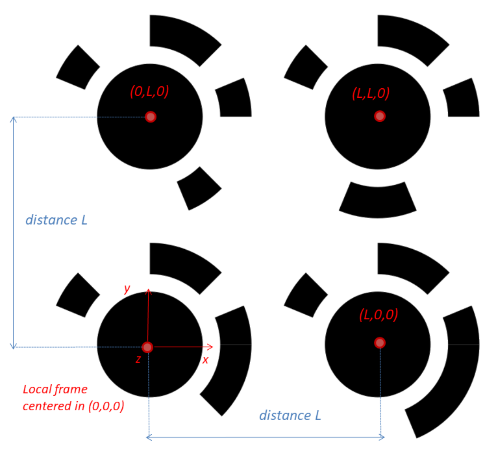
Consider a mobile robot equipped with a monocular camera which tries to localize itself by using coded patterns spread out in its close environment. In our case, each coded pattern is a 2D square surface, composed of four circles of the same size (see
Figure 1). We define the center of the bottom left ellipse as the origin of the pattern’s local frame. In this frame, the
coordinates
of the centers of each ellipse can be computed, knowing the inter-circle distance
L. Consequently, every pattern
j can be fully characterized by:
a rotation matrix between the local frame and a world frame, ;
the position of the origin of the local frame expressed in this world frame, ;
the distance L between the center of two ellipses;
an ID coded by the circular bar-codes.
2.2. Camera Observation Model
At each instant
k, a fiducial pattern detector provides the 2D coordinates of the center of each ellipse,
, associated to the 3D point
of pattern
j in the world frame. According to the pinhole camera model, the reprojection function provides the mathematical relation linking
and
, such as:
with
f being the focal distance of the camera,
being the principal point of the image and parameters
and
, the pixel densities on the horizontal and the vertical axes, respectively.
denotes the
component of vector
. The random process,
, is considered as white Gaussian noise on
with covariance
,
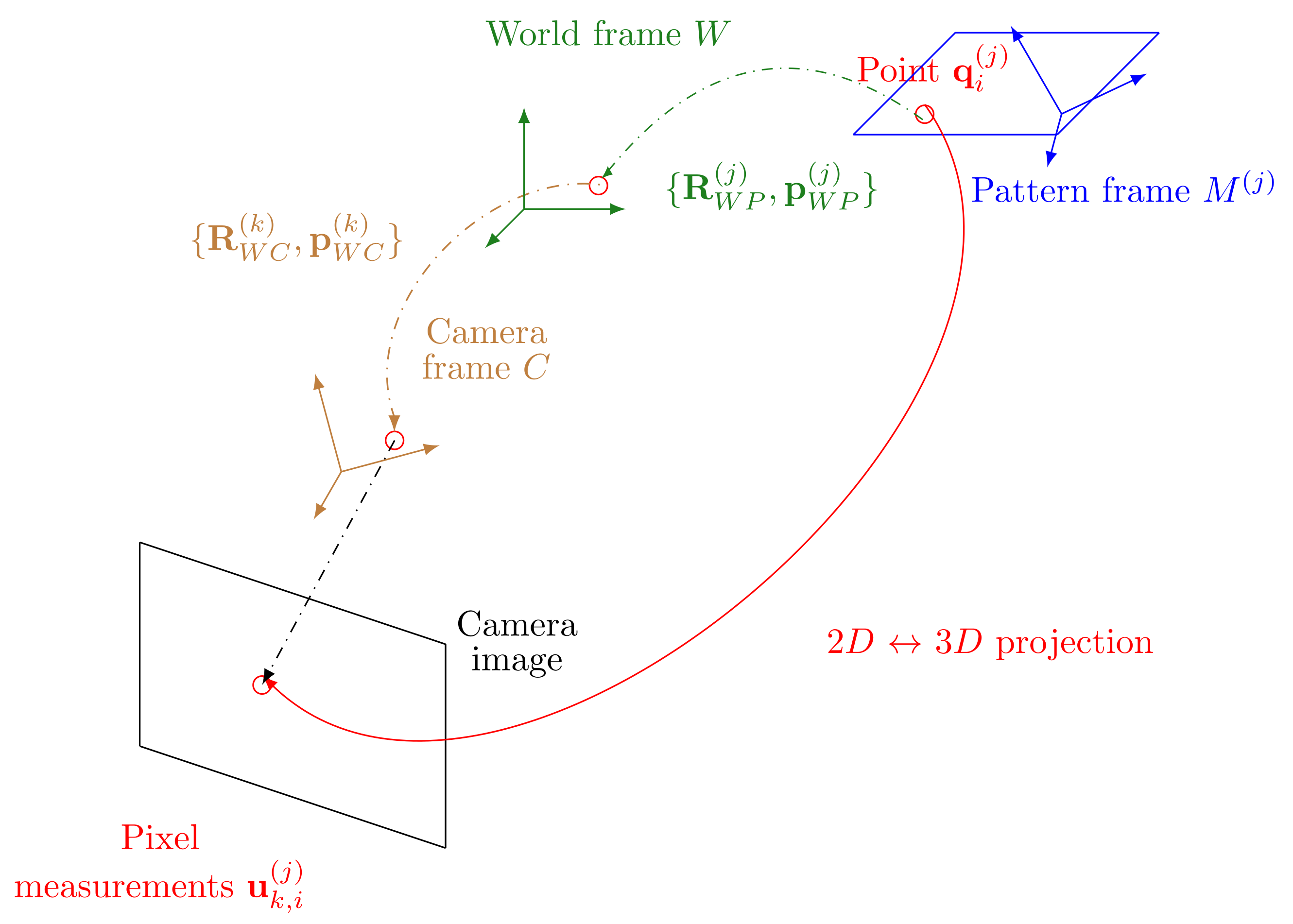
. As illustrated in
Figure 2,
explicitly depends on the rotation matrix
and the rotation between the frame of the coded pattern and the world frame
. In a classical Euclidean framework, they can be parametrized by:
Through this observation model and a given dynamic model, it is possible to estimate the global state containing:
the pose of the camera ;
the set of parameters of the patterns , where K is the number of detected patterns,
by performing a classical EKF-VSLAM [
24].
2.3. Why EKF-SLAM on Lie Groups?
Using the EKF-VSLAM with coded patterns and classical camera model has some drawbacks due to the high non-linearity of the observation model. Indeed, we observe that the unknown variables are linked to the observations by the composition of multiple inverse and trigonometric functions for the Euler parametrization. For the quaternion parametrization, the non-linearity is introduced by the composition of inverse and multiple square functions. Thus, the linearization in the update step of the EKF introduces errors. This can induce some numerical problems in the Jacobian calculation and degrade the performance of the estimation.
In the following, we propose to resolve the SLAM problem by performing the filtering on LGs. Indeed, this formalism enables us to overcome these problems. Particularly:
- •
the camera observation model can be written in a compact way and depends “linearly” on the rotation matrix. Consequently, the approximation at order 1 is more valid;
- •
The Jacobian of the observation model can be computed analytically by considering the geometrical structure of the rotation matrices and does not depend on any parametrization.
3. Background on Lie Groups
3.1. Elementary Notions
A LG
G is a set which has the properties of a group and a smooth manifold [
25,
26]. In this work, we deal with matrix LGs; thus, every element of
G is a matrix belonging to
.
- →
Due to its group structure, G has an internal composition law which is associative. Furthermore, there is an identity element defined, so that each element of the group has an inverse;
- →
Due to its manifold structure, it is possible to compute the derivative and the integral of two elements, or the inverse of one element.
Furthermore, the properties of Lie Groups allow us to define a tangent vector space
at every point
. It is then possible to associate any point of
to any point of
, thanks to the operator called
left tangent application (see
Figure 3). The latter is defined, between two tangent spaces, by:
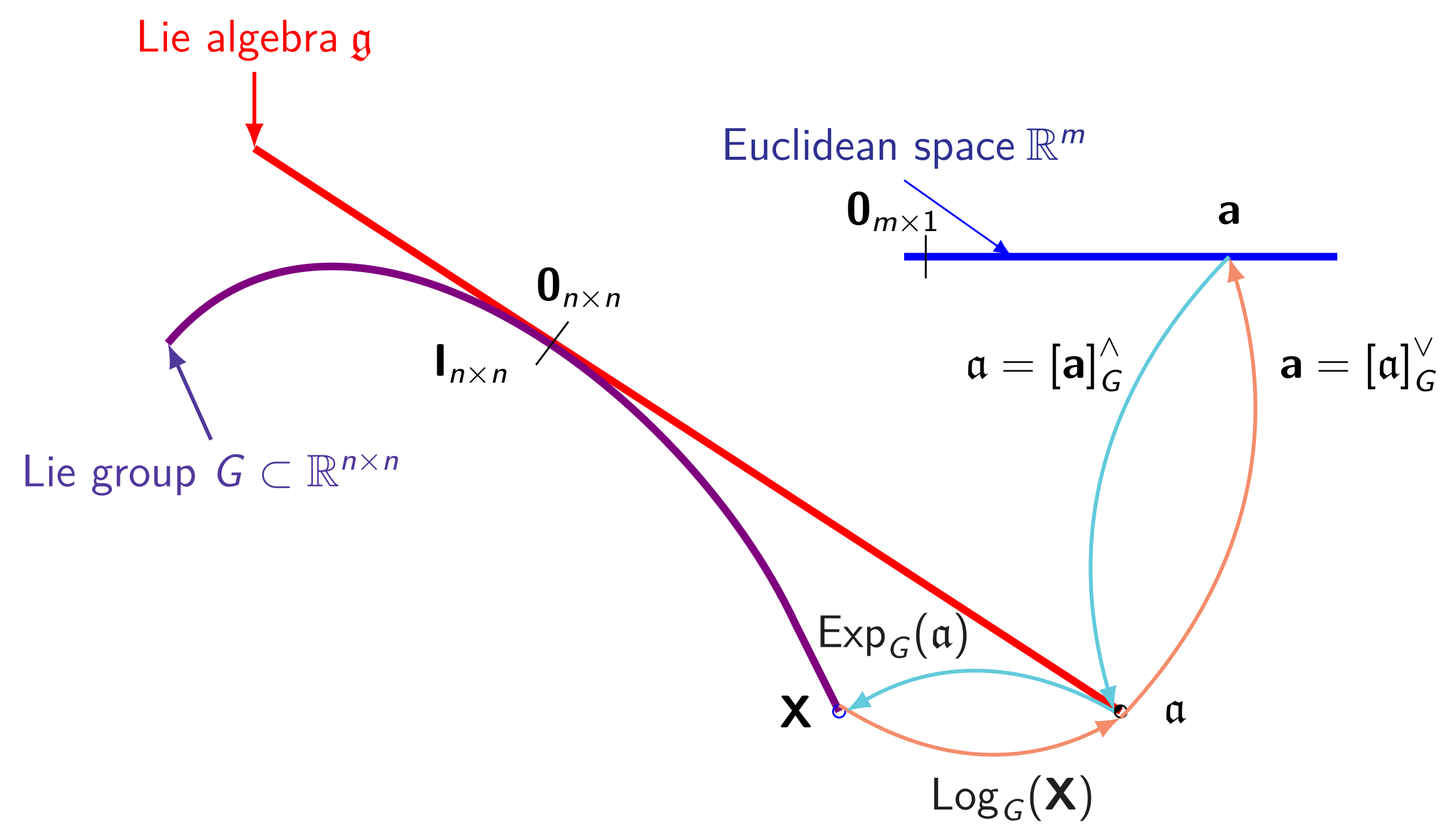
Consequently, we can work with the tangent space to the identity , also called the Lie algebra, denoted as . This space is a vector space with a dimension of m and defines the dimension of G as manifold.
We can establish a relation between
G and
through the exponential mapping,
, and its reciprocal, the logarithm mapping,
. They are locally bijective. The mathematical expressions of these operators can be found in [
25,
27,
28].
On the other hand,
can be directly linked to the Euclidean space
through an isomorphism
and its inverse
, such as
and
,
. To condense these notations, we define
and
, with
and
.
Figure 4 shows, geometrically, the relationship between a LG
G, its Lie algebra
, and
.
3.2. Non-Commutativity and Jacobian
3.2.1. Non-Commutativity
In general, a LG is non-commutative and
:
The adjoint representation allows one to take into account the non-commutativity of LGs. It is an application , such that .
The non-commutativity of LGs can be also explicited through the Baker–Campbell–Hausdorff formula (BCH):
and depends of the left Jacobian matrix, which is written:
where
is an adjoint operator characterizing the non-commutativity directly on the Lie algebra.
3.2.2. Jacobian on LGs
We can define the notion of Jacobian according to a function. Let us consider
an integrable function. We define LG Jacobian of
f by the following expression:
which can be seen as a generalization of the classical directional derivative.
3.3. Lie Groups of Interest
Two useful LGs in our application are introduced in this part.
3.3.1. The Special Orthogonal LG
The LG
is the group of rotation matrices of dimension
n. Every element
of
belongs to the following set:
where
is the determinant of matrix
. Its Lie algebra is the set of skew-symmetric matrices:
where
is the vector of
isomorph to the element of
. The notation
refers to the skew-symmetric matrix operator. In the case of
, every element of
is a 3D rotation matrix, which can be classically parametrized in different ways (quaternions or Euler angles), as seen previously. With the LG formalism, we may parametrize it with an angle vector
. It is written, according to the Rodrigues formula [
29], as:
Every element of its Lie algebra has the following structure:
3.3.2. The Special Euclidean LG
The LG
corresponds to the semi-direct product between
and
:
3.4. Camera Observation Model on LGs
The observation camera model (
1) can be written in a compact way on the LG
. Indeed, the camera rotation
and the associated translation
constitute the rigid-body transformation of the camera and has the following form:
In a similar way for the landmarks, the rotation matrix
and the associated translation
are written as:
According to
Figure 2, we can express the successive
transformations between the camera frame
C and the pattern frame
P in the following way:
Consequently, the pinhole model (
1) can be written as:
where:
and
corresponds to the camera’s calibration matrix:
It is also interesting to note that the model can be written by substituting
L:
where:
This reformulation allows us to define an inverse problem for L. Thus, when the latter is unknown, it is also possible to estimate it conjointly with the camera pose.
4. SLAM Filtering Problem on Lie Groups
In the state-of-the-art VSLAM approaches (Euclidean or Lie groups), the aim is to obtain a recursive estimation of both the pose of the camera and the pose of each pattern in the world frame. The unknown state contains, at each instant, the pose parameters (on
or on
) and the set of 3D points on
. Contrary to the Euclidean VSLAM approach, we propose, in the same way as [
21], to define the pose parameters as a
matrix, but instead of estimating the positions of the 3D points that compose each pattern, we take advantage of the coded patterns approach in order to estimate the
transformation
. Consequently, if the pattern size is known, the estimation of this transformation provides directly the estimation of the 3D position of the center of each ellipse in that pattern. In this way, the global state belongs to several direct products of
. To achieve this estimation, we perform SLAM-extended Kalman filtering on LGs (LG-EKF-VSLAM) based on the LG-EKF proposed in [
23]. Classically, on a Euclidean space, an extended Kalman filter is a recursive filtering algorithm which enables the approximation of the posterior distribution of parameters of interest by a Gaussian distribution. The LG-EKF can be seen as a generalization of the latter in the case where the parameters are lying on LG.
The main difference with the algorithm proposed in [
23] is that we express the landmark initialization phase (mean and covariance) using a concentrated Gaussian on LG.
4.1. Gaussian Distribution on LGs
To perform filtering on LGs, probability distributions on these manifolds have to be defined. Some have already been introduced in the literature, in particular for smooth manifolds [
30,
31]. We focus, in this paper, on the Gaussian distributions (CGD) on LGs, introduced in [
32], which generalizes the concept of Euclidean Gaussian multivariate probability distribution functions (pdf). Indeed, they have similar properties, such as minimizing the entropy under some constraints.
It is possible to obtain a realization from a CGD thanks to a Euclidean Gaussian sample. Indeed, if
is a Gaussian vector with covariance matrix
, and
is a matrix defined on a LG
G of intrinsic dimension
m, then
is distributed according to a left-concentrated Gaussian pdf (CGD) (in a similar way, we can define a right CGD where sample
X can be written
) on
G, with parameters
and
. We note that
. If
is close to
, the expression of this pdf can be approximated by:
where
is the determinant of the matrix
and
is the Mahalanobis distance.
4.2. Unknown State and Evolution Model
The unknown state is constituted of the camera pose and the transformation of every pattern , where is the number of already-detected patterns from an initial instant to instant k.
Due to the dynamics of the robot, some other Euclidean parameters (for instance, the vehicle velocity or the ellipse size) may have to be integrated in the state. Thus, to keep the LG compact in form, such additional parameters can be added into a vector
. Thus, the global state (without landmarks) of our VSLAM problem can be written as:
As a consequence, the LG unknown global state
, containing
and the set of pattern transformations, can be written as:
with
being a square matrix with size
.
To perform the filtering, we have to define the evolution model of this state. By assuming that the patterns are static, the global evolution model can be written as:
where
is a function which expresses the state on the LG
and defines two separated dynamic models on the rotation
and the position
.
- •
is a dynamic evolution function (where corresponds to the dimension of );
- •
is a control input;
- •
, where is a white Gaussian noise on , with covariance matrix .
4.3. Principle of LG-EKF
The aim of the LG-EKF is to recursively approximate the posterior distribution of the unknown parameters defined on LG by a left CGD (note that it also possible to define the LG-EKF-SLAM with a right CGD). Precisely, in our case, we want to approach
by:
where
is the set of all collected measurements from instant 1 to
k. In the same way as the classical EKF, the estimation is done in two steps: prediction and update.
4.3.1. The Prediction Step
The objective of this step is to estimate the distribution
(i.e., estimating the values
), given a prior on the distribution
(defined by
). As
is zero-mean, the prediction of
is given, thanks to the noise-free dynamic model (
30) on LG, by:
and
is given by:
where:
4.3.2. The Update Step
The update step takes advantage of the camera observation
provided at instant
k of the
already-known pattern, in order to approximate:
The parameters
are written as:
where:
and:
is the Jacobian matrix of
:
and
Remark 1. It is important to note that if several patterns are detected at the same instant, the update step is recursively realized for each of them.
4.4. Initialization of Pattern on
If a new pattern is detected by the camera, the step is called the mapping step. As a new object
is detected, the current state
is augmented as follows:
Consequently, the associated covariance to this state can be written as:
where:
At this step, we need to have an initial estimation of the pose of the pattern and of its associated covariance matrix. Classically, in a Euclidean framework, the initialization of a pattern is determined by finding the solution of the inverse of the observation model, and the covariance matrix is approximated by computing correlations using associated Jacobians [
33].
In the case of the camera model, this approach is not feasible due to its analytical complexity, and numeric approaches must be considered. For instance, it is possible to find the initial state by implementing a local bundle adjustment, which optimizes a criterion built from the observation model. The covariance matrix of pattern
j can be obtained by a Gauss–Laplace approximation [
34], and then the global covariance matrix of the new state is updated according to Equation (
39). In this work, we propose an adaptation of this method, using the LG formalism.
The initialization of
can be obtained by minimizing the anti-logarithm (opposite of the logarithm) of the posterior distribution
, associated to the measurement
j. Due to its non-tractability, we propose approaching it by a left CGD with parameters
:
where
is the estimated pose of the new pattern and
its associated covariance.
4.4.1. Computation of
can be determined by maximizing the posterior distribution (
52). Due to the Bayes rule, we show that:
where
is a function conserving the two first components of
. Consequently, we seek to find the minima of the following criterion corresponding to the anti-logarithm of (
54):
where:
and defines an optimization problem on
. A local minima is obtained thanks to a Gauss–Newton algorithm on LG [
35]. At each iteration
l, the updated recursive formula is written as:
where
is a descent direction, computed in the following way:
with:
4.4.2. Computation of
The initial covariance of
is obtained by using a Gauss–Laplace approximation on LG. It consists to approximate
around
under the form:
As
is a critical point of
, we obtain:
By identification, with the expression of the CGD, it implies that
is approximated by:
To obtain the cross-correlation matrix
, as in (
51), we perform an update step of the increased state (
50) with the measurement
.
5. Experiments
In this section, we compare our proposed approach, the LG-EKF-VSLAM, to the standard EKF-VSLAM algorithm while using coded patterns. We first carried out two Monte-Carlo simulations in order to evaluate the usefulness of performing LG modelling for monocular visual SLAM. In the first scenario, we considered that the distance between the center of two ellipse on the coded patterns, L, is perfectly known. For the second simulation, L is added to the state vector as a parameter to be estimated.
We then evaluated the LG-EKF-VSLAM with real data obtained within our laboratory, since, to the best of our knowledge, there are no available public benchmarks with coded patterns.
5.1. Experiments with Simulated Data
In the simulated scenarios, we considered a wheeled robot following a trajectory generated according to a constant velocity model. The control input is given by a simulated angular velocity
. The unknown state is constituted of the camera pose
and the linear velocity
:
The discrete dynamic model is written as:
where
is the sampling rate.
,
, and
are four white Gaussian noises on linear and angular velocity, position, and orientation, respectively. These equations can be written on
G with the form (
30), where:
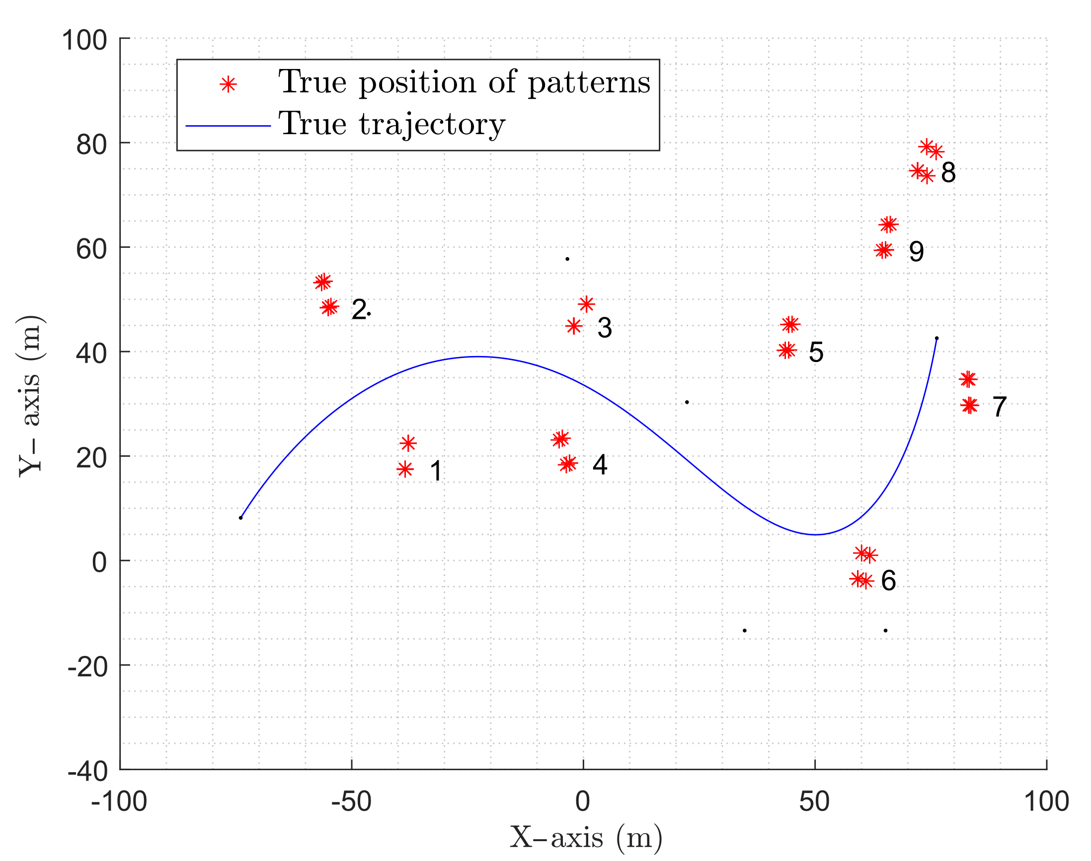
The obtained trajectory is generated during
with
, and is shown in
Figure 5. The positions of each coded pattern are defined with a null z-axis and are randomly distributed all along the ground-truth trajectory. Their orientations are obtained by sampling from a CGD on
, with mean
and covariance
.
The camera measurements are simulated according to the model (
22), with:
The Jacobian matrices
,
, and
of the LG-EKF-VSLAM (from Equations (
7), (
35), and (
47), respectively) have been implemented according to the formulation given in
Appendix A.1,
Appendix B, and
Appendix C.
The performance of the method must be evaluated on a state belonging to . Consequently, we studied it by separating the estimator associated with the rotation matrix and the estimator associated with the position .
- (1)
The quality of can be evaluated by using two intrinsic metrics on LGs, which enables us to compute the rotation error directly on :
- •
a RMSE (Root Mean Square Error) metric, which can be seen as a generalization of the classical Euclidean RMSE. The classical distance is substituted by the geodesic distance on
[
36]:
where
corresponds to the Monte-Carlo realization
i of the rotation matrix estimator at epoch
k.
is the number of realizations;
- •
a mean RPE (Relative Pose Error) metric to evaluate the relative pose error between two consecutive epochs for several realizations of the algorithm.
- (2)
As the position parameter is Euclidean, the quality of its estimator is determined with the classical Euclidean RPE and RMSE.
These performances are compared to a Euclidean EKF-VSLAM. In the latter, the rotation matrix is parametrized by Euler angles . Consequently, the unknown state is a vector which belongs to . The estimation error on rotation and position are directly evaluated by a classical RPE and RMSE between the vector and the estimated vector .
5.1.1. Case 1: L Perfectly Known
According to
Table 1, we observe that the proposed method slightly outperforms the classical EKF-VSLAM. Two arguments can explain these results:
Firstly, the LG modelling takes into account the intrinsic properties of the unknown state belonging to . Consequently, the indeterminacy of the Euler angle estimates is deleted;
Secondly, through this modelling, the observation model is freed from the non-linearity introduced by the cosine and sine functions of the rotation matrix in the Euclidean modelling. In this way, the approximation of the covariance estimation error is more precise.
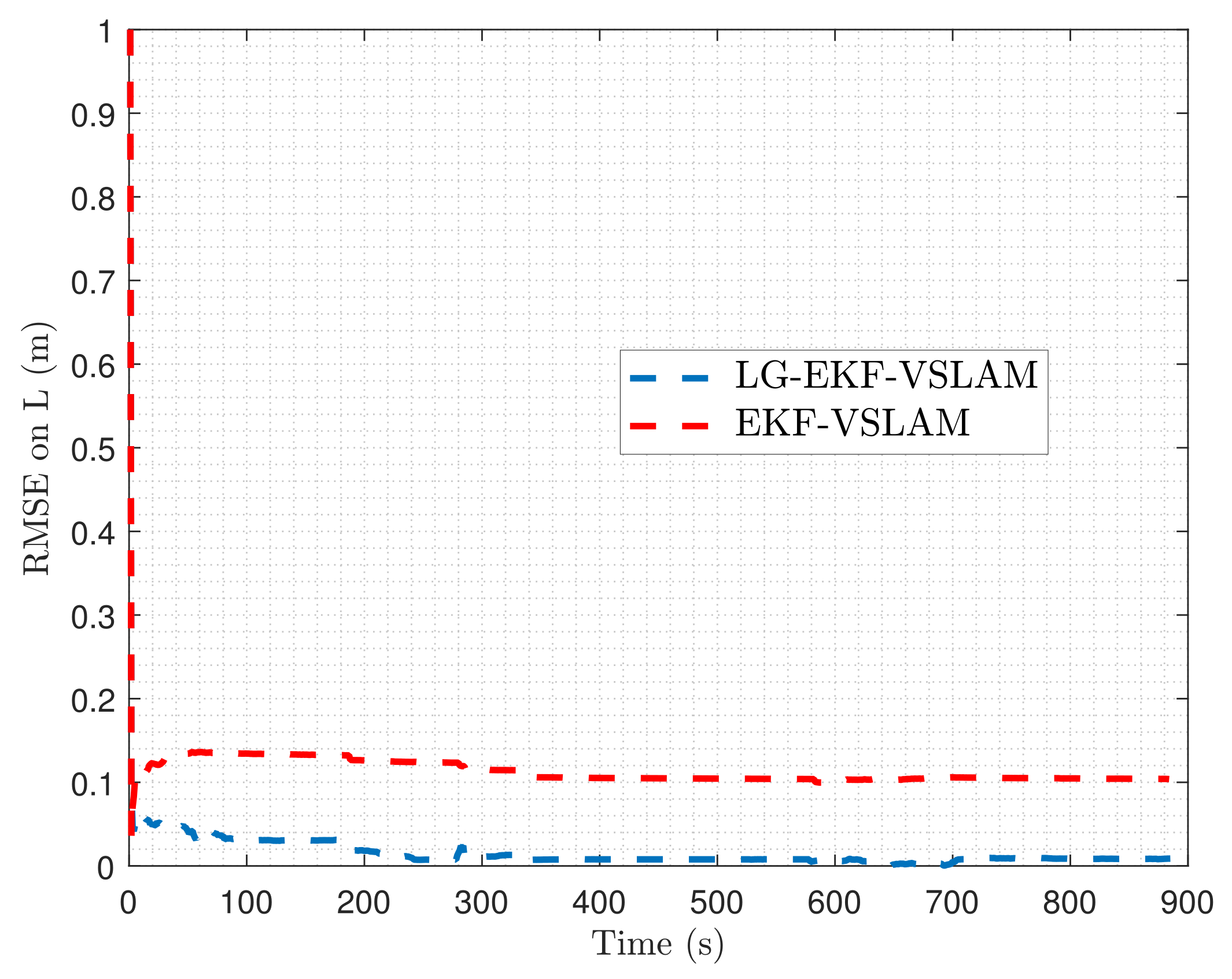
5.1.2. Case 2: L Is Misspecified
In order to challenge the proposed algorithm, we assume that the distance between two ellipses of a pattern is incorrectly specified. Consequently,
L is initialized with an initial error on the true value (5 m) equal to 1 m, and added to the state:
In order to estimate L with the LG-EKF-VSLAM, the observation model that explicitly involves L is considered. From a numerical point of view, we also have to compute the Jacobian of the observation model according to L.
From the obtained results given in
Table 2 and
Figure 6, we can observe that the LG-EKF-VSLAM achieves the best results. Indeed, compared to the EKF-VSLAM, it is able to asymptotically converge to the true value of
L, in spite of high initialization errors (here,
. Indeed, the estimation error becomes inferior to
. Moreover, the precision of the estimator, after convergence, is better than for the Euclidean EKF-VSLAM (see
Table 2).
5.2. Experiment with Real Data
5.2.1. Experiment Setup
To validate the methodology presented in the previous section (
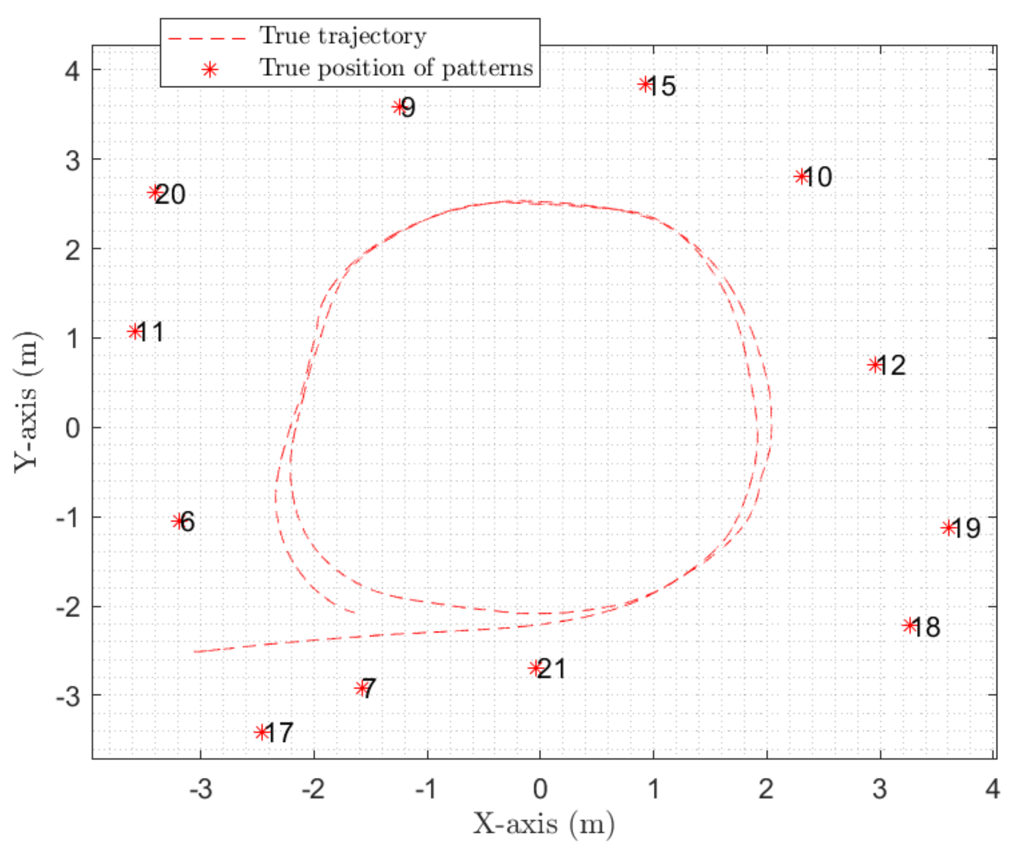
Section 4), we performed an experiment with a monocular camera (PointGrey Blackfly from Flir @7fps), with a 3.8–13-mm Varifocal lens, embedded on a mobile cart. Additionally, an Optitrack motion-capture system provided the ground truth for the pose of the camera and the coded patterns. The camera’s reference trajectory and the true positions of the coded patterns (i.e., the center of the bottom-left ellipse) are represented in Figure 8. The camera’s calibration matrix is given by:
In this experiment, 12 coded patterns, each printed on a
paper, with
, were placed in different places of the room, as illustrated in
Figure 7 and
Figure 8. The camera moved in a circular motion and the fiducial pattern-detection algorithm provided observations for each frame. The state
contains the pose, but also the linear and angular velocity
. Indeed, in our experiment, no angular sensor is available; thus, we used a constant velocity model. Consequently, we have:
To take into account the circular motion of the mobile in the filter, we propose leveraging a position-prediction model correlating its position and orientation. Indeed, the correlations between these two variables are especially high in the turns.
The proposed model has the following structure:
The translation velocity and rotation matrix are assumed to follow the evolution models (
66) and (
68). Moreover, we suppose that the angular velocity follows a random walk process with a Gaussian white noise
. Consequently, the function
is written as:
The computation of the Jacobian of
is provided in
Appendix A.2.
5.2.2. Obtained Results
In order to use the method with real data, we first have to define the noise parameters. Concerning the observation model, the covariance noise is taken to be sufficiently high in order to take into account the uncertainties introduced by non-analytical phenomenons. Consequently, we take with pixels. Concerning the dynamic model, the standard deviation of noises , , , and are, respectively, fixed at , , and .
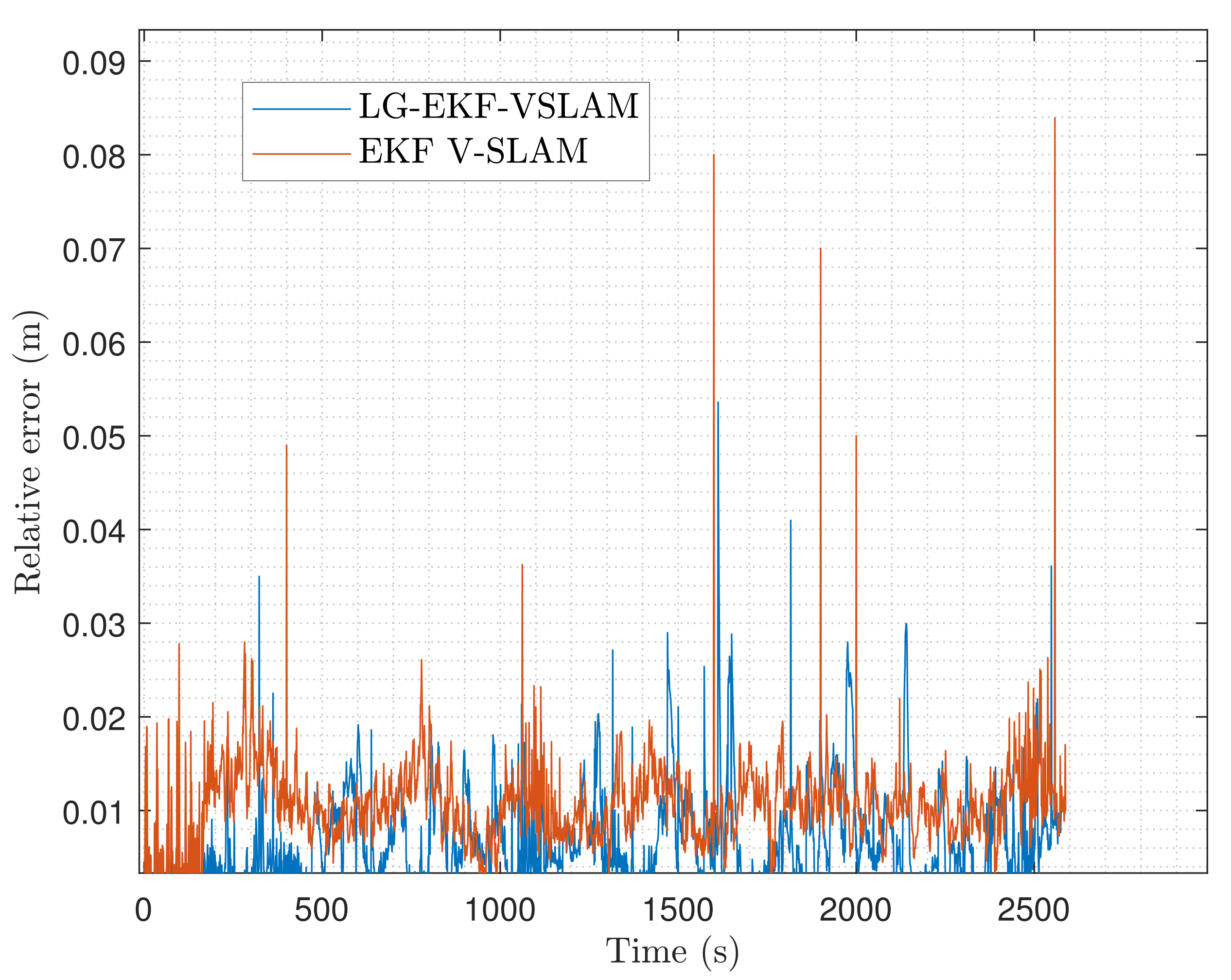
In order to quantify the estimation error of the trajectory, we use the Optitrack reference system and compare it with the estimated trajectory given by each of the two methods. This is done by computing the absolute error on the position at each instant of the trajectory, as represented in
Figure 9.
In the two approaches, we first observe, through the
Figure 10 and
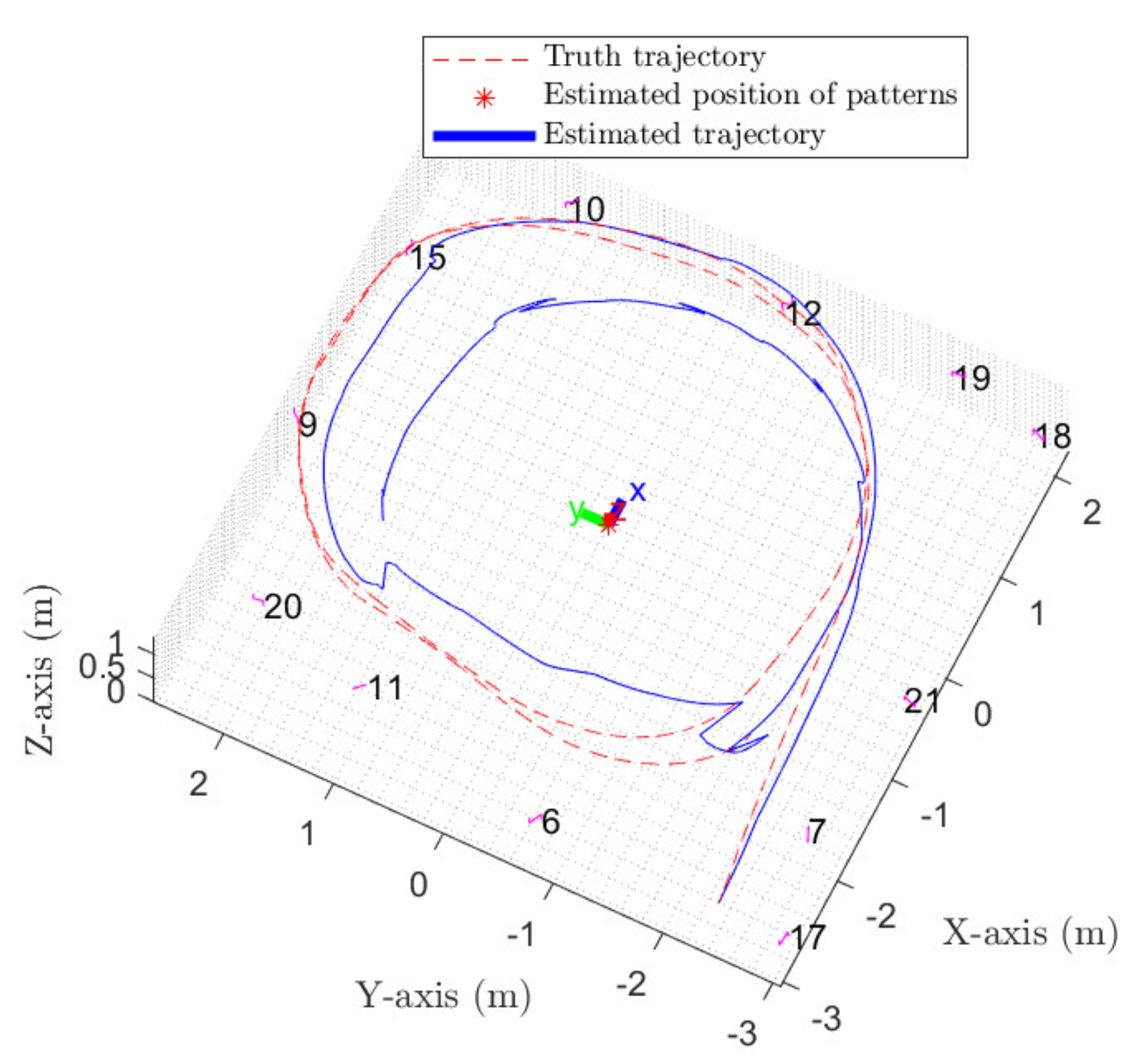
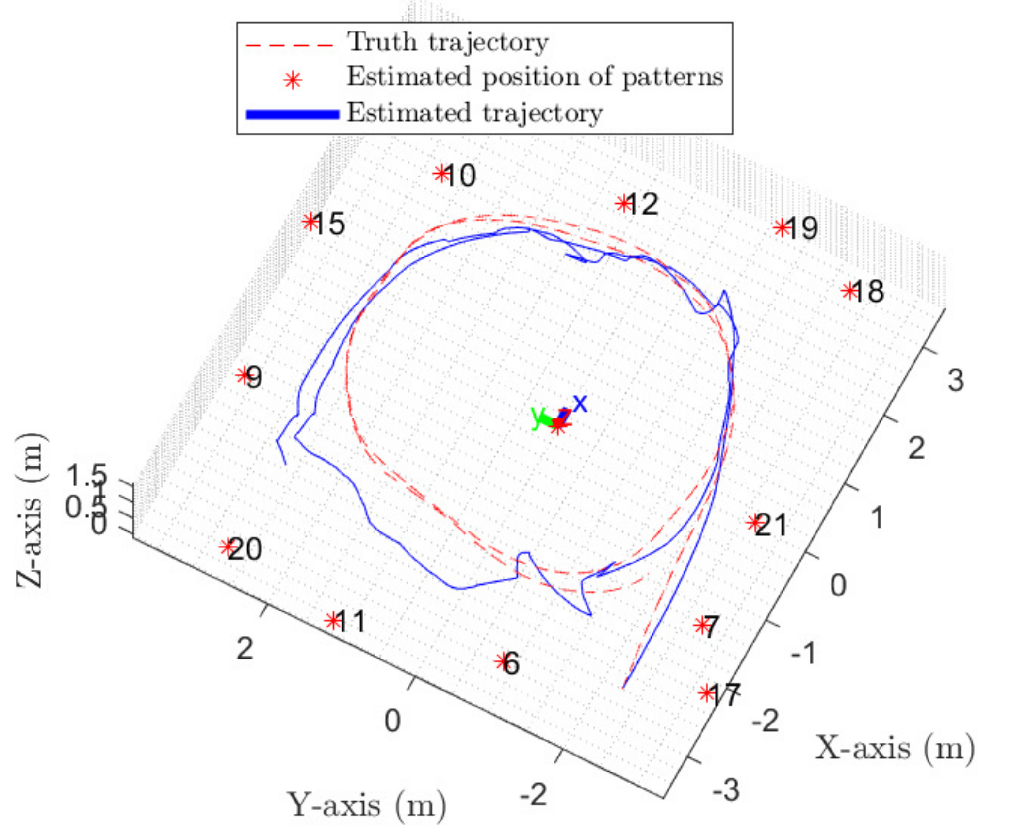
Figure 11, that the estimated position is particularly degraded in some parts of the trajectory, especially between the coded patterns 9 and 11 and 6 and 7. This is due to the pattern detector, which does not provide any detection because of blur and specular reflection on the objects. Consequently, during these instants, the estimation is only realized by dead-reckoning navigation, and the non-linearities of the models increases the pose-estimation error. In
Figure 9, we observe that the performance of the two approaches are quite similar in terms of absolute error estimation, even if the LG-EKF-VSLAM performs a little bit better all over the trajectory. This is confirmed through
Figure 11. Indeed, we observe that during the last turn of the trajectory, the EKF-VSLAM tends to deviate from the ground truth, implying a higher estimation error.
6. Conclusions
In this paper, we propose an original modelling on LGs in order to perform monocular VSLAM. After reformulating the classical pinhole on LGs, we propose a EKF-VSLAM algorithm on LG for coded-pattern landmarks. We take into account the particularity of the SLAM problem by proposing a LG method to initialize new patterns. Our algorithm has been compared with a classical EKF-VSLAM using a Euler parametrization on simulated data as well as on real-world data. Both the simulation and the experiments showed the validity and the performance improvement provided by the proposed LG-EKF-VSLAM, compared to the state-of-the-art solution. In addition, we have shown that a misspecified value on the size of the coded pattern has a large impact on the estimation solution. When this parameter is taken into account as a new state in the estimation process, the EKF-VSLAM reduces the estimation error, but is outperformed by the LG-EKF-VSLAM, which converges asymptotically to the true value of L. This is mostly due to the LG formalism, which copes better with system non-linearities.
A pertinent perspective would be to propose a LG-based approach by taking into account the lack of knowledge of non-estimated parameters models. In our case,
L could be considered uncertain, but not estimated. There exist Euclidean filtering approaches dedicated to this problem [
37]; consequently, it would be pertinent to adapt them for parameters lying on LGs.
Moreover, in a general way, it would be interesting to adapt the formalism of LG (especially the optimization method) to other applications in computer vision and signal processing. For instance, we can quote the well-known problems of Structure of Motion (SfM) [
38] and image registration [
39].
From an application point of view, another perspective would be to fuse the camera measurements with, for instance, information from Ultra-Wide-Band sensors or with a Global Navigation Satellite System for outdoor navigation, in order to improve the performance of the algorithm, especially in situations where camera frames can be lost or where no patterns are present in the close environment of the vehicle.
Author Contributions
Conceptualization, S.L. and D.V.; methodology, S.L.; S.L. designed the models; writing—original draft preparation, S.L.; writing—review and editing, S.L., G.P. and D.V.; experiments were designed by G.P. and D.V., and were equally realized with S.L.; supervision, G.P. and D.V.; project administration, G.P.; funding acquisition, G.P. All authors have read and agreed to the published version of the manuscript.
Funding
This research was funded by the DGA/AID (French Secretary of Defense) under grant n 2018.60.0072.00.470.75.01.
Institutional Review Board Statement
Not applicable.
Informed Consent Statement
Informed consent was obtained from all subjects involved in the study.
Data Availability Statement
The data presented in this study are available on request to the corresponding author. The data belong to ISAE-SUPAERO and are not publicly available.
Conflicts of Interest
The authors declare no conflict of interest. The funders had no role in the design of the study; in the collection, analyses, or interpretation of data; in the writing of the manuscript, or in the decision to publish the results.
Appendix A. Computation of C(k−1)
It should be remembered that:
Appendix A.1. Case of from (69)
We know that
is defined by:
Consequently, the Jacobian of
, according to
, is written as:
with:
Due to the structure of
, we show that:
Appendix A.2. Case of from (78)
We know that
is defined by:
The Jacobian has the following structure:
where
and
are defined by (A4), (A5), and (A6). We show that:
where
is a vector basis of Lie algebra
.
Appendix B. Computation of J(k)
It should be remembered that:
Consequently, we have to compute two quantities: and .
Appendix B.1. Computation of
corresponds to the Jacobian of the observation, according to
. Consequently:
In order to compute this Jacobian, we need to know:
- •
the classical derivative product rule according to ;
- •
the fact that , where is the lth vector basis of Lie algebra .
Consequently, by computing:
can be obtained in the following way:
is, thus, obtained thanks to the product rule:
with:
Appendix B.2. Computation of
corresponds to the Jacobian of the observation, according to
. Thus:
By using the classical derivative product rule, according to
, we obtain:
Thus,
is given by:
Appendix C. Expression of
Appendix C.1. Case of SO(3)
The left Jacobian of
is given by the following expression [
26]:
Appendix C.2. Case of SE(3)
The left Jacobian of
is given by the following expression [
32]:
with
and
Appendix C.3. Case of G
In our case, the LG of interest is written as
, such that:
with
. As
is a commutative LG,
. Furthermore,
is the block diagonal concatenation of
repetitions of
.
References
- Engel, J.; Schöps, T.; Cremers, D. LSD-SLAM: Large-Scale Direct Monocular SLAM. In Computer Vision—ECCV 2014, Proceedings of the 13th European Conference, Zurich, Switzerland, 6–12 September 2014; Springer International Publishing: Cham, Switzerland, 2014; pp. 834–849. [Google Scholar]
- Khairuddin, A.R.; Talib, M.S.; Haron, H. Review on simultaneous localization and mapping (SLAM). In Proceedings of the IEEE International Conference on Control System, Computing and Engineering, Penang, Malaysia, 27–29 November 2015; pp. 85–90. [Google Scholar]
- Triggs, B.; McLauchlan, P.; Hartley, R.; Fitzgibbon, A. Bundle Adjustment—A Modern Synthesis. In Proceedings of the International Workshop on Vision Algorithms, Corfu, Greece, 21–22 September 1999. [Google Scholar]
- Mouragnon, E.; Lhuillier, M.; Dhome, M.; Dekeyser, F.; Sayd, P. 3D reconstruction of complex structures with bundle adjustment: An incremental approach. In Proceedings of the 2006 IEEE International Conference on Robotics and Automation, Orlando, FL, USA, 15–19 May 2006; pp. 3055–3061. [Google Scholar]
- Guivant, J.; Nebot, E. Optimization of the simultaneous localization and map-building algorithm for real-time implementation. IEEE Trans. Robot. Autom. 2001, 17, 242–257. [Google Scholar] [CrossRef] [Green Version]
- Harris, C.; Stephens, M. A combined corner and edge detector. In Proceedings of the Fourth Alvey Vision Conference, Manchester, UK, 31 August–2 September 1988; pp. 147–151. [Google Scholar]
- Rosten, E.; Drummond, T. Machine learning for high-speed corner detection. In Proceedings of the European Conference on Computer Vision, Graz, Austria, 7–13 May 2006. [Google Scholar]
- Bowman, S.L.; Atanasov, N.; Daniilidis, K.; Pappas, G.J. Probabilistic data association for semantic SLAM. In Proceedings of the 2017 IEEE International Conference on Robotics and Automation (ICRA), Singapore, 29 May–3 June 2017; pp. 1722–1729. [Google Scholar]
- Lim, H.; Lee, Y.S. Real-time single camera SLAM using fiducial markers. In Proceedings of the ICCAS-SICE, Fukuoka, Japan, 18–21 August 2009; pp. 177–182. [Google Scholar]
- Houben, S.; Droeschel, D.; Behnke, S. Joint 3D laser and visual fiducial marker based SLAM for a micro aerial vehicle. In Proceedings of the IEEE International Conference on Multisensor Fusion and Integration for Intelligent Systems (MFI), Baden-Baden, Germany, 19–21 September 2016; pp. 609–614. [Google Scholar]
- Kalaitzakis, M.; Cain, B.; Carroll, S.; Ambrosi, A.; Whitehead, C.; Vitzilaios, N. Fiducial Markers for Pose Estimation Overview, Applications and Experimental Comparison of the ARTag, AprilTag, ArUco and STag Markers. J. Intell. Robot. Syst. 2021, 101, 71. [Google Scholar] [CrossRef]
- Fiala, M. ARTag, a fiducial marker system using digital techniques. In Proceedings of the 2005 IEEE Computer Society Conference on Computer Vision and Pattern Recognition, San Diego, CA, USA, 20–25 June 2005; Volume 2, pp. 590–596. [Google Scholar]
- Pilté, M.; Bonnabel, S.; Barbaresco, F. Tracking the Frenet-Serret frame associated to a highly maneuvering target in 3D. In Proceedings of the 2017 IEEE 56th Annual Conference on Decision and Control (CDC), Melbourne, VIC, Australia, 12–15 December 2017; pp. 1969–1974. [Google Scholar]
- Mika, D.; Jozwik, J. Lie groups methods in blind signal processing. Sensors 2020, 20, 440. [Google Scholar] [CrossRef] [PubMed] [Green Version]
- Bourmaud, G.; Giremus, A.; Berthoumieu, Y.; Mégret, R. Discrete Extended Kalman Filter on Lie groups. In Proceedings of the EUSIPCO, Marrakech, Morocco, 9–13 September 2013. [Google Scholar]
- Bonnabel, S.; Martin, P.; Salaün, E. Invariant Extended Kalman Filter: Theory and application to a velocity-aided attitude estimation problem. In Proceedings of the 48h IEEE Conference on Decision and Control (CDC) held jointly with 2009 28th Chinese Control Conference, Shanghai, China, 15–18 December 2009; pp. 1297–1304. [Google Scholar]
- Wang, J.; Zhang, C.; Wu, J.; Liu, M. An Improved Invariant Kalman Filter for Lie Groups Attitude Dynamics with Heavy-Tailed Process Noise. Machines 2021, 9, 182. [Google Scholar] [CrossRef]
- Brossard, M.; Bonnabel, S.; Condomines, J.P. Unscented Kalman filtering on Lie groups. In Proceedings of the 2017 IEEE/RSJ International Conference on Intelligent Robots and Systems (IROS), Vancouver, BC, Canada, 24–28 September 2017; pp. 2485–2491. [Google Scholar]
- Ćesić, J.; Marković, I.; Bukal, M.; Petrović, I. Extended information filter on matrix Lie groups. Automatica 2017, 82, 226–234. [Google Scholar] [CrossRef]
- Marjanovic, G.; Solo, V. An engineer’s guide to particle filtering on matrix Lie groups. In Proceedings of the 2016 IEEE International Conference on Acoustics, Speech and Signal Processing (ICASSP), Shanghai, China, 20–25 March 2016; pp. 3969–3973. [Google Scholar]
- Brossard, M.; Bonnabel, S.; Barrau, A. Invariant Kalman Filtering for Visual Inertial SLAM. In Proceedings of the 2018 21st International Conference on Information Fusion (FUSION), Cambridge, UK, 10–13 July 2018; pp. 2021–2028. [Google Scholar]
- Lenac, K.; Marković, I.; Petrović, I. Exactly sparse delayed state filter on Lie groups for long-term pose graph SLAM. Int. J. Robot. Res. 2018, 37, 585–610. [Google Scholar] [CrossRef]
- Bourmaud, G.; Mégret, R. Robust large scale monocular visual SLAM. In Proceedings of the 2015 IEEE Conference on Computer Vision and Pattern Recognition (CVPR), Boston, MA, USA, 7–12 June 2015; pp. 1638–1647. [Google Scholar]
- Hui, C.; Shiwei, M. Visual SLAM based on EKF filtering algorithm from omnidirectional camera. In Proceedings of the 2013 IEEE 11th International Conference on Electronic Measurement Instruments, Harbin, China, 16–19 August 2013; Volume 2, pp. 660–663. [Google Scholar]
- Selig, J.M. Geometrical Methods in Robotics; Springer: Berlin/Heidelberg, Germany, 1996. [Google Scholar]
- Solà, J.; Deray, J.; Atchuthan, D. A micro Lie theory for state estimation in robotics. arXiv 2018, arXiv:1812.01537. [Google Scholar]
- Faraut, J. Analysis on Lie Groups: An Introduction; Cambridge University Press: Cambridge, UK, 2008. [Google Scholar]
- Chirikjian, G. Information-Theoretic Inequalities On Unimodular Lie Groups. J. Geom. Mech. 2010, 2, 119–158. [Google Scholar] [CrossRef] [PubMed]
- Koks, D. A Roundabout Route to Geometric Algebra. In Explorations in Mathematical Physics: The Concepts Behind an Elegant Language; Springer Science: Berlin/Heidelberg, Germany, 2006; Chapter 4; pp. 147–184. [Google Scholar]
- Said, S.; Bombrun, L.; Berthoumieu, Y.; Manton, J.H. Riemannian Gaussian Distributions on the Space of Symmetric Positive Definite Matrices. IEEE Trans. Inf. Theory 2017, 63, 2153–2170. [Google Scholar] [CrossRef] [Green Version]
- Pennec, X. Intrinsic statistics on Riemannian manifolds: Basic tools for geometric measurements. J. Math. Imaging Vis. 2006, 25, 127–155. [Google Scholar] [CrossRef] [Green Version]
- Barfoot, T.; Furgale, P.T. Associating Uncertainty With Three-Dimensional Poses For Use In Estimation Problem. IEEE Trans. Robot. 2014, 30, 679–693. [Google Scholar] [CrossRef]
- Sola, J.; Monin, A.; Devy, M.; Lemaire, T. Undelayed initialization in bearing only SLAM. In Proceedings of the 2005 IEEE/RSJ International Conference on Intelligent Robots and Systems, Edmonton, AB, Canada, 2–6 August 2005; pp. 2499–2504. [Google Scholar]
- Bishop, C. Pattern Recognition and Machine Learning; Springer: Berlin/Heidelberg, Germany, 2006. [Google Scholar]
- Bourmaud, G.; Mégret, R.; Giremus, A.; Berthoumieu, Y. From Intrinsic Optimization to Iterated Extended Kalman Filtering on Lie Groups. J. Math. Imaging Vis. 2016, 55, 284–303. [Google Scholar] [CrossRef] [Green Version]
- Huynh, D.Q. Metrics for 3D Rotations: Comparison and Analysis. J. Math. Imaging Vis. 2009, 35, 155–164. [Google Scholar] [CrossRef]
- Chauchat, P.; Vilà-Valls, J.; Chaumette, E. Robust Linearly Constrained Invariant Filtering for a Class of Mismatched Nonlinear Systems. IEEE Control Syst. Lett. 2022, 6, 223–228. [Google Scholar] [CrossRef]
- Ozyesil, O.; Voroninski, V.; Basri, R.; Singer, A. A Survey of Structure from Motion. Acta Numerica 2017, 26, 305–364. [Google Scholar] [CrossRef]
- Zitová, B.; Flusser, J. Image registration methods: A survey. Image Vis. Comput. 2003, 21, 977–1000. [Google Scholar] [CrossRef] [Green Version]
Figure 1.
Representation of the coded pattern and its local frame. The detection algorithm detects the red points , , , and .
Figure 1.
Representation of the coded pattern and its local frame. The detection algorithm detects the red points , , , and .
Figure 2.
Geometrical representation of the projection camera model.
Figure 2.
Geometrical representation of the projection camera model.
Figure 3.
Geometrical relationship between and through the left tangent application.
Figure 3.
Geometrical relationship between and through the left tangent application.
Figure 4.
Relation between the Lie group, the Lie algebra, and the Euclidean space. For each element , we associate an element in Lie algebra, which is converted in a element of LG G, thanks to the operator .
Figure 4.
Relation between the Lie group, the Lie algebra, and the Euclidean space. For each element , we associate an element in Lie algebra, which is converted in a element of LG G, thanks to the operator .
Figure 5.
Simulated true trajectory and ellipse center positions of 9 coded labelled patterns.
Figure 5.
Simulated true trajectory and ellipse center positions of 9 coded labelled patterns.
Figure 6.
Evolution of the RMSE on L for realizations.
Figure 6.
Evolution of the RMSE on L for realizations.
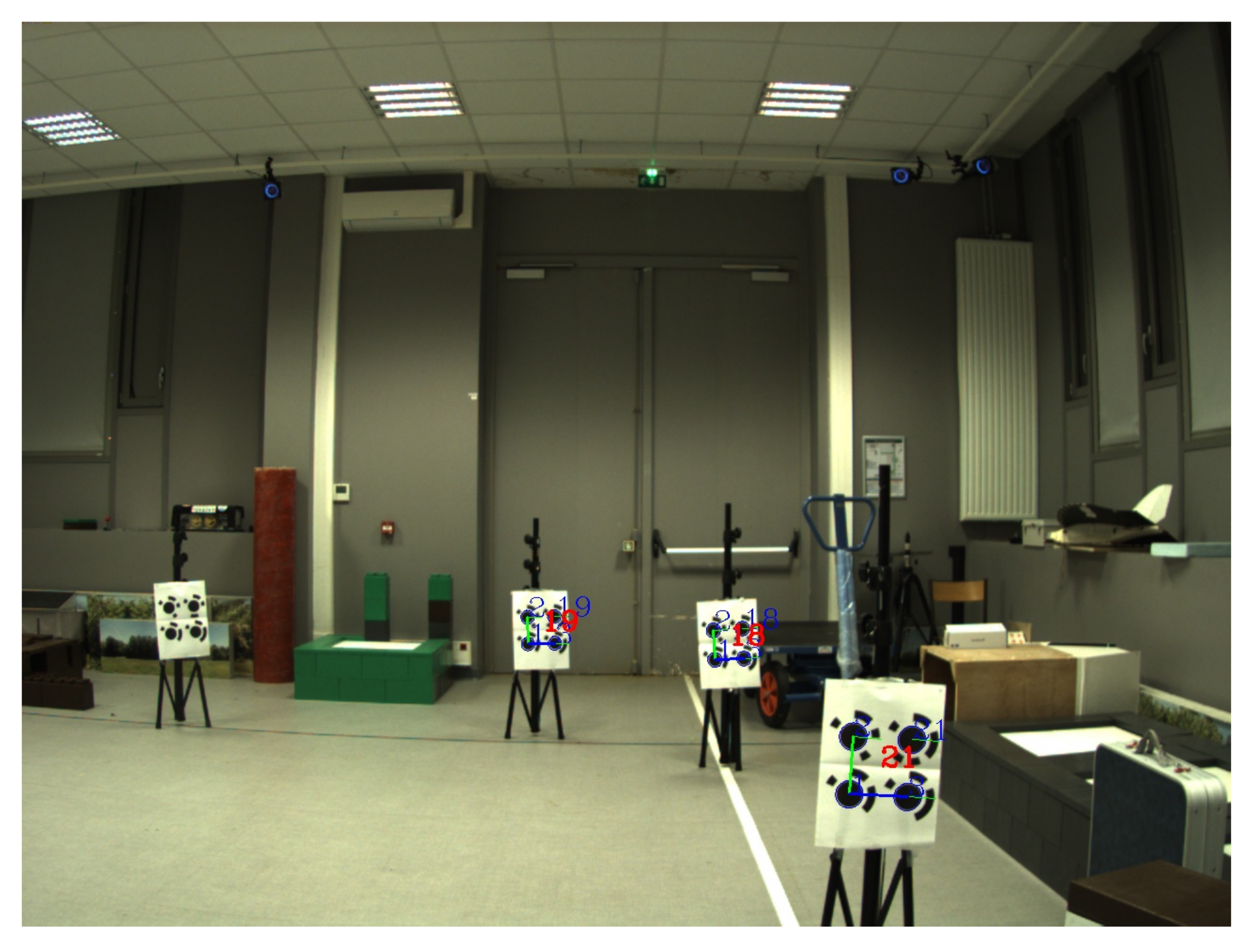
Figure 7.
First image frame integrated in the detector: it computes the ellipse coordinates of the pattern with labels 18, 19, and 21.
Figure 7.
First image frame integrated in the detector: it computes the ellipse coordinates of the pattern with labels 18, 19, and 21.
Figure 8.
Ground truth obtained by an Optitrack motion capture system in the XY–plane, superimposed to the position of the center of the bottom-left ellipse of each coded pattern.
Figure 8.
Ground truth obtained by an Optitrack motion capture system in the XY–plane, superimposed to the position of the center of the bottom-left ellipse of each coded pattern.
Figure 9.
Absolute position error obtained for the two methods.
Figure 9.
Absolute position error obtained for the two methods.
Figure 10.
Estimated trajectory for EKF–VSLAM.
Figure 10.
Estimated trajectory for EKF–VSLAM.
Figure 11.
Estimated trajectory for LG–EKF–VSLAM.
Figure 11.
Estimated trajectory for LG–EKF–VSLAM.
Table 1.
Simulation results with known L. Obtained performance estimation for realizations.
Table 1.
Simulation results with known L. Obtained performance estimation for realizations.
| | LG-EKF-VSLAM | EKF-VSLAM |
|---|
| RMSE position (m) | 0.298 | 0.427 |
| RMSE orientation (rad) | 0.0048 | 0.0055 |
| RPE position (m) | 0.0172 | 0.0205 |
| RPE orientation (rad) | | |
Table 2.
Simulation results with misspecified L. Obtained performance estimation for realizations.
Table 2.
Simulation results with misspecified L. Obtained performance estimation for realizations.
| | LG-EKF-VSLAM | EKF-VSLAM |
|---|
| RMSE position (m) | 0.758 | 1.257 |
| RMSE orientation (rad) | 0.0158 | 0.065 |
| RPE position (m) | 0.0398 | 0.0924 |
| RPE orientation (rad) | | |
| Publisher’s Note: MDPI stays neutral with regard to jurisdictional claims in published maps and institutional affiliations. |
© 2022 by the authors. Licensee MDPI, Basel, Switzerland. This article is an open access article distributed under the terms and conditions of the Creative Commons Attribution (CC BY) license (https://creativecommons.org/licenses/by/4.0/).


