Article

Wetland Vegetation Classification through Multi-Dimensional Feature Time Series Remote Sensing Images Using Mahalanobis Distance-Based Dynamic Time Warping

College of Oceanography and Space Informatics, China University of Petroleum (East China), Qingdao 266580, China
*
Author to whom correspondence should be addressed.
Remote Sens. 2022, 14(3), 501; https://doi.org/10.3390/rs14030501
Submission received: 28 November 2021 / Revised: 19 January 2022 / Accepted: 20 January 2022 / Published: 21 January 2022
(This article belongs to the Special Issue Advanced Earth Observations of Forest and Wetland Environment)

Abstract

:
Efficient methodologies for vegetation-type mapping are significant for wetland’s management practices and monitoring. Nowadays, dynamic time warping (DTW) based on remote sensing time series has been successfully applied to vegetation classification. However, most of the previous related studies only focused on Normalized Difference Vegetation Index (NDVI) time series while ignoring multiple features in each period image. In order to further improve the accuracy of wetland vegetation classification, Mahalanobis Distance-based Dynamic Time Warping (MDDTW) using multi-dimensional feature time series was employed in this research. This method extends the traditional DTW algorithm based on single-dimensional features to multi-dimensional features and solves the problem of calculating similarity distance between multi-dimensional feature time series. Vegetation classification experiments were carried out in the Yellow River Delta (YRD). Compared with different classification methods, the results show that the K-Nearest Neighbors (KNN) algorithm based on MDDTW (KNN-MDDTW) has achieved better classification accuracy; the overall accuracy is more than 90%, and kappa is more than 0.9.

1. Introduction

Wetlands are one of the most important and biologically diverse ecosystems on earth, providing numerous essential ecosystem services and representing significant economic value [1]. Wetland vegetation, as an important component of wetland ecosystems, plays an important role in biodiversity conservation [2,3], climate regulation [4], and water conservation [5]. The knowledge of the geospatial distribution of vegetation is paramount to support high levels of biodiversity and provide a wide range of ecosystem services in wetland. The Yellow River Delta (YRD) reserve is the largest natural vegetation area of new wetland along the coast of China, which has been challenged by climate change and alien vegetation invasion in recent years, and some plant communities are facing significant threats [6]. Therefore, wetland monitoring and mapping has become the key to protecting the ecological environment of the region. However, traditional wetland plant community mapping requires intensive field work, which is labor intensive, expensive, time consuming, and sometimes not applicable due to limited accessibility. Fortunately, remote sensing technology provides a powerful tool for identifying and mapping wetland plant communities in large areas [7,8].
With the improvement of the spatial and temporal resolution of satellite remote sensing, time series remote sensing images have played an important role in land cover mapping and other fields [9,10,11,12]. The accessibility of multitemporal satellite images could reduce the impact on classification caused by the complexity of surfaces and, to some extent, the similarity between the spectrum of different vegetation [13]. However, part of the image is occluded by clouds and fog, resulting in missing data values [14,15], and the inconsistency of the input data dimensions makes it difficult to apply conventional classifiers, which need consistent data dimensions. In addition, time series remote sensing images have proven to be of great value to acquire phenological insights for land cover mapping, which is reflected by vegetation indexes [16,17]. Some data fitting methods, such as Linear fitting [18] and Fourier transform [19,20,21], were used to fit vegetation growth curves and extract phenological features for classification [22,23,24,25], but the periodicity of vegetation is vulnerable to climate, and the time of plant growth and withering may be delayed or advanced [26,27,28], which affects the classification results.
The dynamic time warping (DTW) algorithm, which was first applied to speech and pseudo signature recognition, has been proven to be an effective solution to deal with the time series challenges described above [29,30]. As an algorithm widely used for time series matching, this method finds the minimum distance of time series to measure the similarity between two time series by stretching or shrinking distorted time series [31], and the partial data values could be overcome. Although the DTW method can make full use of all time information for better time series shape matching, it ignores the time range, which is a troublesome issue for vegetation classification with similar time series shape but different phenological cycles. In response to this shortcoming, some scholars have introduced time constraints and proposed time-weighted dynamic time warping (TWDTW) to help distinguish different types of land cover categories. This avoids the false matching caused by time delay considering the time offset of vegetation phenological characteristics [32,33,34]. This method has been widely used in crop phenological information extraction and mapping, forest tree species classification, etc.
At present, the time series analysis method based on DTW has been successfully applied to the field of vegetation classification; unfortunately, most of the relevant studies are based on a single vegetation index such as Normalized Difference Vegetation Index (NDVI) or Enhanced Vegetation Index (EVI) [35,36]. Plants have obvious spectral reflection characteristics, which are closely related to their development, health, and growth conditions. Making full use of spectral information in complex wetland environments is very important for vegetation classification. For example, paper [37] extracted a variety of spectral indices combined with DTW for classification. However, this method uses each time point as a vector to calculate its Euclidean distance in the DTW local distance, which is also DTW based on Euclidean distance (EDDTW), and assigns the same weight to each feature while ignoring the relationship between different features [38,39]. On the one hand, the time series with multiple features should be considered as a whole in order to maintain the correlation between features [40]. On the other hand, different features may be subject to various interferences or have nothing to do with the final classification results, and there are differences between features. Therefore, how to calculate the overall time series similarity distance and maintain the relationship between different features is the focus of research in time series classification with multiple features.
In this study, Mahalanobis Distance-based Dynamic Time Warping (MDDTW) was proposed to solve the problem of calculating the distance of multi-dimensional feature time series. This method extends the traditional time series similarity calculation based on single features to a multi-dimensional feature time series, and effectively combines multiple vegetation indexes for wetland vegetation classification. Specifically, this study combined multiple spectral indexes to construct multi-dimensional feature time series, then calculated similarity distance with MDDTW. Finally, the Random Forest (RF) algorithm and the K-Nearest Neighbors (KNN) algorithm, based on distance measurement, was carried out in wetland vegetation classification mapping. There are many abbreviations in this study, which are summarized in Appendix A.

2. Materials and Methods

2.1. Study Area

The Yellow River Delta (118°33′–119°20′ E, 37°35′–38°12′ N) is located in the Shandong Peninsula. The study area, approximately 50 square kilometers, is shown in Figure 1. Located in the land-sea transition zone at the estuary of the Yellow River, the YRD is about to be ranked as one of the most intact, largest, and the most juvenile wetland ecosystems on the planet [41]. It is also the largest natural vegetation area of newborn wetland along the coast of China, with an abundance of natural plants resources. The halophyte community that consists of Phragmites australis (P. australis), Robinia pseudoacacia (R. pseudoacacia), Suaeda salsa (S. salsa), Tamarix chinensis (T. chinensis), Salix matsudana (S. matsudana), and Spartina alterniflora (S. alterniflora), is the main biocoenosis in the study area. Furthermore, there are many farmlands on the edge of the study area, which will be classified as a vegetation type in this study because crops are similar to wetland halophytes and have a certain growth cycle.

2.2. Data Set

2.2.1. Remote Sensing Data

The Sentinel-2 MSI data used in this study were from the European Space Agency’s Sentinel Scientific Data Hub. The Sentinel-2 consists of two identical satellites, namely Sentinel-2A and Sentinel-2B, allowing a 5-day revisit time at the equator and an even shorter time toward the poles. As a system suitable for monitoring vegetation growth, the Sentinel-2 records the reflected radiance in 13 spectral bands covering the visible and near-infrared to the short-wave infrared spectrum, with a spatial resolution as high as 10 m. The data were the top-of-atmosphere (TOA) reflectance after orthophoto correction and geometric fine correction. In order to avoid the interference of cloud, 31 images with less cloud cover were selected, and the image dates obtained are shown in Table 1.

2.2.2. Field Survey Data

Compared with the landlocked environment, natural coastal wetland environments are complex and variable. In order to better understand the spatial distribution of vegetation communities, researchers conducted a field expedition of wetland vegetation groups in the YRD from 20 September to 30 September 2019.
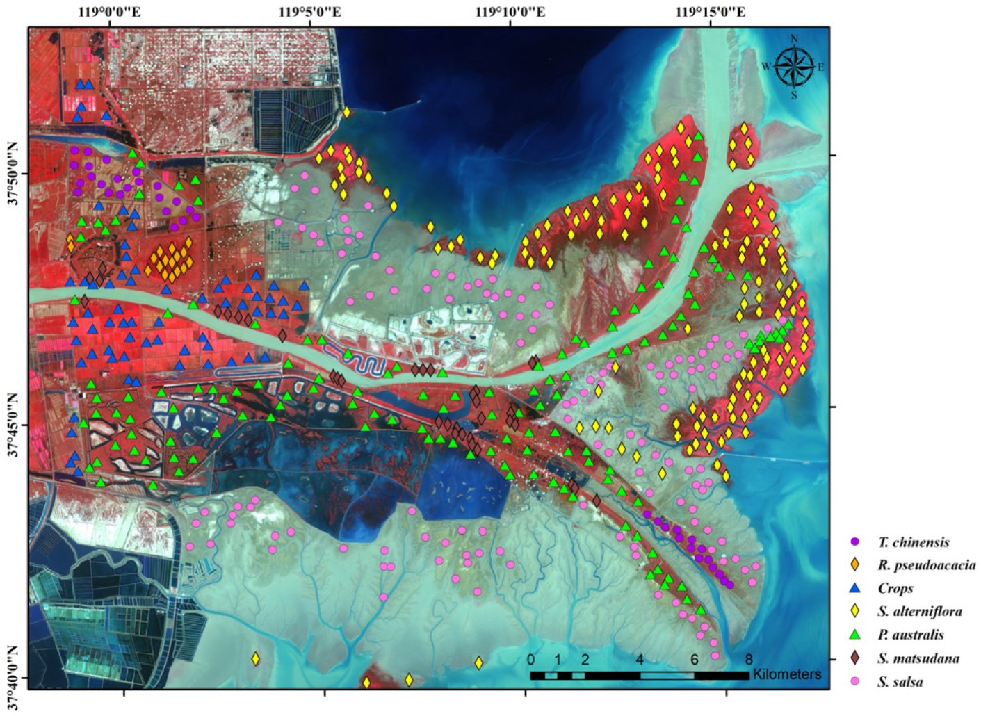
There are 116 field stations, which can be seen as calibration points in this investigation, whose distribution is shown in Figure 2. Furthermore, UAV aerial photography was used to obtain information regarding 574 validation points in three areas that are difficult for personnel to reach: natural tidal beach area, semi closed area affected by S. alterniflora, and fully closed tidal flat. The collection of field survey data could be used as a reference for selecting training samples and validation samples.
The distribution of validation points covers the vegetation growth area, as shown in Figure 3. In the remote sensing image, pixel points of 3 × 3 window size with each point as the center are selected, and the vegetation of different pixels in the same window is guaranteed to be the same, which reduces the influence of positioning error. The final classification results are evaluated by validation pixel points in combination with the field survey data. It should be noted that the calibration points and validation points selected in the experiment are completely independent and their sites are different.

2.3. Data Preprocessing

Preprocessing is required because the Sentinel-2 Level-1C products in this research are top-of-atmosphere radiance. Firstly, all images were subjected to radiometric calibration and atmospheric correction to obtain surface reflectance, employing the Sen2Cor algorithm [42] using SNAP software. The Fmask4.0 [43] model in MATLAB software was then used to set the pixels affected by cloud as invalid pixels because the pixels of the original image can be cloud-contaminated. Finally, the Sentinel-2 satellite images were clipped to extract the study area.
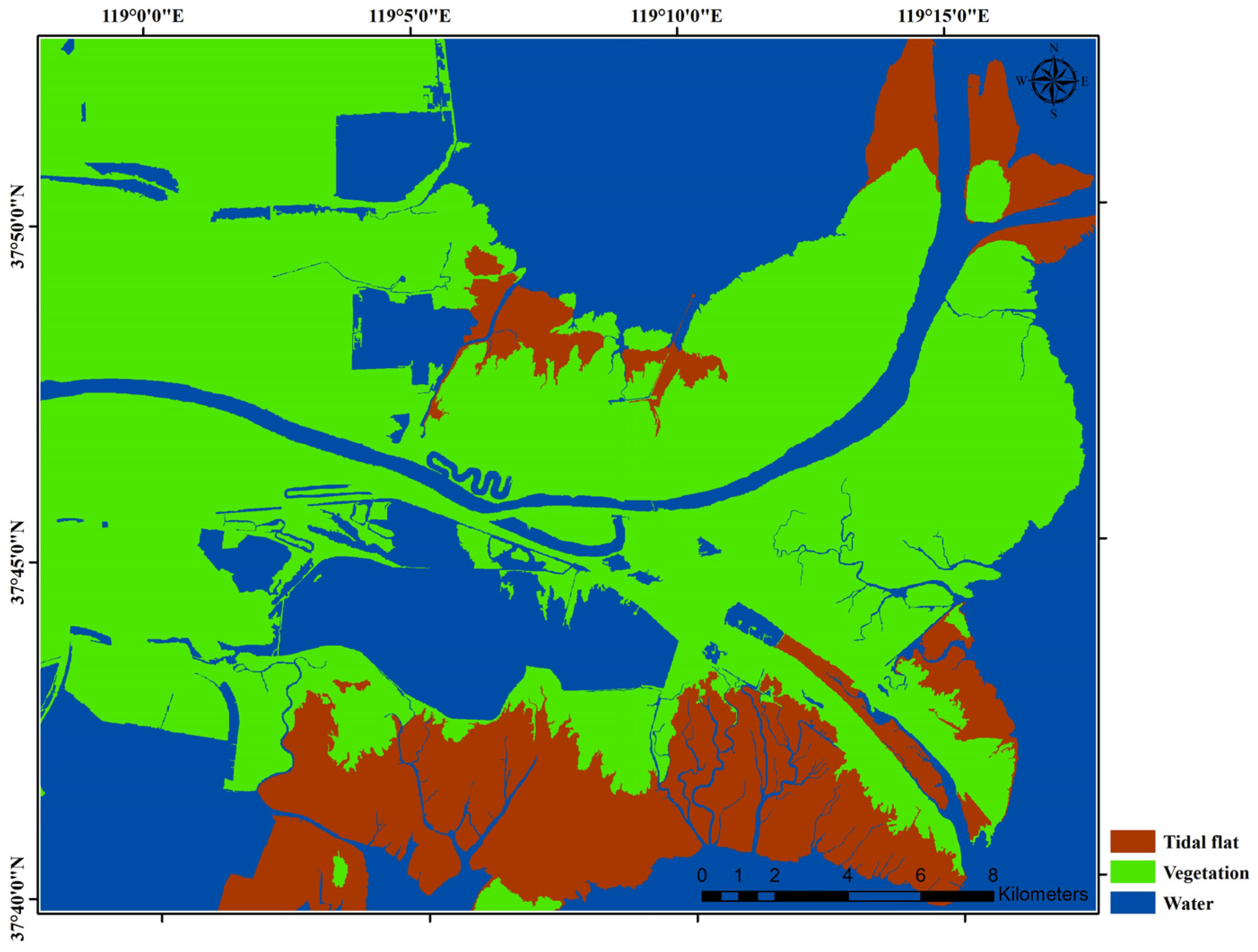
The land cover types in the study area are complex, because there are many non-vegetated areas such as bare tidal flat and water. However, this study mainly focuses on the classification of vegetation using its time series. Extracting the vegetation covered area is the top priority of vegetation classification. Because the vegetation grows vigorously in September, when the image has fewer clouds and fog, a single decision tree was used to generate the surface classification for the image of 29 September to classify water, vegetation, and tidal flat with the support of eCognition software, which contains a variety of multi-scale segmentation methods. The classification results of the ground surface are shown in Figure 4. It should be pointed out that the automatic classification results are manually edited in combination with the survey data to ensure the accuracy of extracting the vegetation coverage area as much as possible. In the experiment, classification is only carried out in the vegetation area.

2.4. Methods

In this study, four vegetation index features (NDVI, DVI, EVI, RVI) were extracted based on Sentinel-2 data to first construct multi-dimensional feature time series. The Mahalanobis distance was then used to extend the DTW algorithm-based one-dimensional features to multi-dimensional features for calculating the similarity distance of multi-dimensional feature time series. Because the traditional Mahalanobis distance based on the covariance of the sample set could not accurately measure the sample similarity relationship, this study uses metric learning to train the Mahalanobis matrix and then solve the similarity distance. Finally, the KNN classifier was used to classify wetland vegetation. The overall steps of the experiment are shown in Figure 5.

2.4.1. Multi-Dimensional Feature Time Series

The Ratio Vegetation Index (RVI) is the earliest vegetation index [44], which strengthens the difference between vegetation in the infrared band and the near-infrared band. However, it does not consider the influence of atmospheric and soil factors. The EVI [45] has a high sensitivity for vegetation, especially for high vegetation cover, and reduces the interference of soil area and atmospheric factors. The Difference Vegetation Index (DVI) [46] is sensitive to vegetation with medium and low coverage. The NDVI is one of the most widely used vegetation indexes, and is also the most commonly used index to monitor plant growth status. Based on these analyses, four common vegetation indices (NDVI, DVI, EVI, RVI) were extracted to build multi-dimensional time series. It is important to point out that different features can be developed for classification, including but not limited to the above four.
The vegetation indices were calculated by the following Equations (1)–(4).
R V I = ρ R E D ρ N I R
E V I = G × ( ρ N I R ρ R E D ) ( ρ N I R + C 1 × ρ R E D C 2 × ρ B L U E + L )
D V I = ρ N I R ρ R E D
N D V I = ρ N I R ρ R E D ρ N I R + ρ R E D
where, ρ N I R represents the near-infrared band reflectance and ρ B L U E is the spectral reflectance of the blue band, while ρ R E D represents the red band reflectance. As for EVI, G is the gain factor, which was set to 2.5. L is the background adjustment factor, which was set to 1. Furthermore, C 1 and C 2 are adjustment factors for fit; in this study, C 1 was set to 6 and C 2 was set to 7.5.

2.4.2. Mahalanobis Distance-Based DTW (MDDTW)

DTW is an algorithm based on the idea of dynamic programming; it is commonly used to measure the similarity of two time series of different lengths and was initially applied to problems involving template matching [47,48]. It has been widely cited in the analysis of time series remote sensing data processing in recent years [49]. The algorithm uses the time warping function, satisfying certain conditions to describe the time correspondence between the standard time series features and the time series features to be matched. According to the warping path corresponding to the minimum cumulative distance when the two-time series features are matched, the similarity of different time series is measured, and the DTW distance is obtained.
Two time series data, X and Y, are expressed as:
  X =   x 1 ,   x 2 ,   x 3 ,   ,   x m   Y =   y 1 ,   y 2 ,   y 3 ,   ,   y n
where m and n are the lengths of X and Y.
In order to calculate the DTW distance, a matrix of m × n is constructed according to the time series X and Y, where elements (i, j) represent the relative distance, d(xi, yj), between the two points xi and yi in the corresponding sequences. The data on sequence Y are nonlinearly mapped to sequence X.
The optimal warp path W is expressed as:
W =   w 1 , w 2 , , w k , , w K
where max ( m , n ) K m + n 1 . The path satisfies the following constraints: boundary, continuity, and monotonicity [50]. The main aim is to find the only optimal path among many bending distances that minimizes the cumulative optimal distance, as shown in Figure 6.
The final DTW distance is calculated according to Equation (7).
  r ( i , j ) = d ( i , j ) + min [ r ( i 1 , j 1 ) , r ( i 1 , j ) , r ( i , j 1 ) ]   DTW ( X , Y ) = min { r ( m , n ) }
where r ( i , j ) represents the cumulative distance, which is the cumulative minimum distance from the starting point (1,1) to the end point ( i , j ) , and r ( 1 , 1 ) = D M X 1 , Y 1 . The local distance measure, d ( i , j ) , is defined as:
d ( i , j ) = ( x i y i ) 2
For the multi-dimensional feature time series constructed by NDVI, DVI, EVI, and RVI, different index features will be given the same weight, and the correlation between features will be ignored if the Euclidean distance is chosen to calculate the DTW local distance. As mentioned above, features have different correlation with the label of subjects, and there might also be correlations between the different features. A feasible strategy is to use the Mahalanobis distance function to measure the local distance of vectors in multi-dimensional feature time series.
Mahalanobis distance was designed to measure the distance between a distribution and a single point [51], and it is an effective method to calculate the similarity of two unknown sample sets, using the Mahalanobis matrix to calculate the correlation between variables.
Two multi-dimensional time series X and Y are expressed as:
X = x 11 x 12 x 1 m x 21 x 22 x 2 m x d 1 x d 2 x d m Y = y 11 y 12 y 1 n y 21 y 22 y 2 n y d 1 y d 2 y d n
where d is the dimension of the multi-feature time series, and m and n represent the length of multi-dimensional time series X and Y, respectively.
The local distance in DTW is calculated by the Mahalanobis distance as Equation (10),
D M X i , Y j   = X i Y j T M X i Y j
where X i = ( x 1 i , x 2 i , , x d i ) T , 1 i m represents the ith column of X, which is the value of each variable at time i; Y j = ( y 1 j , y 2 j , , y d j ) T , 1 j n represents the jth column of Y, which is the value of each variable at time j. The PSD matrix, M, is named as the Mahalanobis matrix.
The dynamic time warping algorithm is expressed as:
  r ( i , j ) = D M X i , Y j   +   min { r ( i 1 , j ) , r ( i , j 1 ) , r ( i 1 , j 1 ) }   DTW M ( X , Y ) = min { r ( m , n ) }
where r ( i , j ) is the cumulative minimum distance from (1,1) to ( i , j ) , and r ( 1 , 1 ) = D M X 1 , Y 1 .
Through the above theoretical derivation, a new measure called MDDTW is formed, combining Mahalanobis distance and DTW, which represent the similarity of multi-dimensional characteristic time series. How to obtain the appropriate Mahalanobis distance is a key problem in this study. The traditional Mahalanobis distance is generally obtained based on the inverse of the covariance matrix, which represents the relationship of the internal aggregation of data. However, it is not enough that the measurement distance function can only reflect the internal aggregation relationship of data. More importantly, it is necessary to establish the relationship between sample attributes and categories. Therefore, a metric learning method is employed for Mahalanobis distance learning to calculate the similarity of multi-dimensional characteristic time series in this study.

2.4.3. Metric Learning for MDDTW

In the study of metric learning, Mahalanobis distance is no longer simply limited to the inverse of the covariance matrix, but needs to be obtained through the process of metric learning [52]. The purpose of metric learning based on Mahalanobis distance is to obtain a positive semi-definite symmetric matrix, M, for a given training sample set, X, to establish the relationship between the eigenvectors of the samples. In this way, the similar relationship between the training samples is preserved, and the distance of the same samples is closer, while different kinds are distant. The paper [53,54] developed a new Mahalanobis distance metric learning algorithm using triple constraint and information entropy, and it succeeded in image processing and pattern recognition. Therefore, this method is employed in this study.
Applying the LogDet divergence as the regularization term, the LogDet divergence-based metric learning model [55,56] for multi-dimensional features time series is expressed as:
M t + 1 = arg min M 0 D l d M , M t   +   η t 𝓁 M , y ^ t , y t
where M t is the Mahalanobis matrix of the tth iteration and η t represents a regularization parameter, which satisfies η t > 0 to balance D l d M , M t and 𝓁 M , y ^ t , y t .
D l d M , M t is the regularization function, which is expressed as:
D l d M , M t   = tr M M t 1     log det M M t 1     n
𝓁 M , y ^ t , y t is the loss function, which is expressed as:
𝓁 M , y ^ t , y t   = max 0 , ρ + d M x i , x j     d M x i , x k
where y ^ t represents the predicted value, y t represents the expected value, and d M is the Mahalanobis distance of two samples. The three samples x i , x j , x k in the sample set constitute a set of triple constraints, and x i , x j , x k represent multi-dimensional feature time series and belong to two different categories, respectively.
The final solution result of M is expressed as Equation (15) through mathematical derivation [57,58], while q t M t q t T p t M t p t T < ρ   .
M t + 1 = γ t + η t γ t q t T t T γ t 1     η t q t T γ t q t η t = α t r I     M t 1 M t q t q t T γ t = M t η t M t p t p t T M t 1   +   η t p t T M t p t
where p t =   x i x j ; q t =   x i x k , and α is a constant learning rate parameter, which is chosen between 0 and 1. When the M is obtained by metric learning, the similarity distance of multi-dimensional feature time series can be calculated by MDDTW. In the later stage of this study, a KNN algorithm suitable for distance measurement is combined for vegetation classification.
In the vegetation covered area, each pixel position is time-expanded, and the Ma-halanobis matrix (M) is obtained by using the metric learning method described as above. Because the triple constraint needs to be rebuilt whenever M is updated, the number of cycles for setting the dynamic triple constraint construction strategy is set to 10. In each cycle, the number of ternary constraints is N = 5n, where n is the number of training samples. In the later stage of this study, a KNN algorithm suitable for distance measurement is combined for vegetation classification.

3. Experiment and Results

In order to verify the effectiveness of the classification method based on MDDTW, this study compared four classification methods, including Random Forest based on multitemporal (RF-Multitemporal), Random Forest based on pixel-differential time series (RF-PDTS), TWDTW, and EDDTW. Section 3.1 mainly explains the experimental details and the parameter settings of different classification methods. The classification maps of the different methods are shown in Section 3.2.

3.1. Experiment

For the classification based on MDDTW, RF, and KNN, the classifiers were employed after calculating the distance of multi-dimensional features by the MDDTW method. For RF classifiers, the number parameter of classifiers is set to 10 and the depth of decision tree is 50. For the KNN classifier, the distance between each pixel and the samples was calculated directly and then classified. In this study, the K was set to 1 after many experimental comparisons. It should be noted that parallel processing was used to improve efficiency during the KNN classifier employed. As for the EDDTW, which is similar to MDDTW, the time series is constructed by combining four vegetation indexes. Different time points are regarded as vectors, and the local distance of DTW is calculated by Euclidean distance [59]. The RF and KNN classifiers were used for classification, and the parameter settings are the same as for MDDTW. For the classification based on RF-Multitemporal, the remote sensing images of the four seasons of spring, summer, autumn, and winter are selected as the data to be classified, as shown in Figure 7; this can reflect the seasonal difference and ensure that the vegetation area is cloudless. The number of Random Forest classifiers is set to 10, and the depth of the decision tree is 50.
For the RF-PDTS [25], the number of Random Forest classifiers is set to 10 and the depth of the decision tree is 50.
TWDTW constrains time by setting weights and takes into account the seasonal changes of land cover types. It is an advanced time series classification method [60], where α (gain factor) and β (time distance) are important weight parameters. In this study, α = 0.25 and β = 45 were determined based on experiments, as shown in Figure 8. The RF and KNN classifiers are used for classification, respectively, and are the same as the MDDTW parameters settings.

3.2. Result

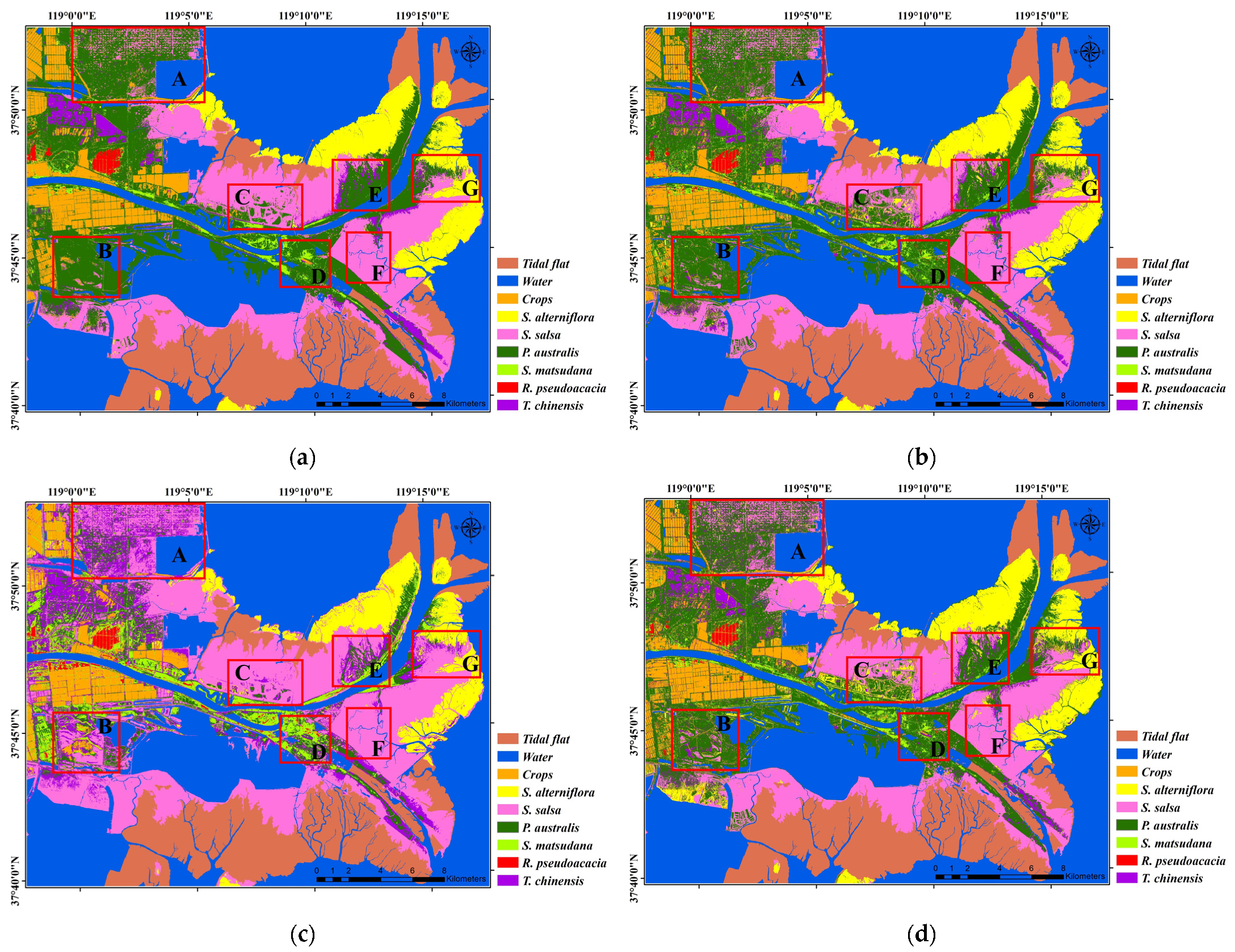
The classification results based on multitemporal Random Forest, RF-PDTS, TWDTW, EDDTW, and MDDTW are shown in Figure 9a–h. For crops S. alterniflora, R. pseudoacacia, and T. chinensis, different classification maps have spatial consistency, and the distribution of those is roughly the same. Seven areas, A–G, where classified maps have obvious differences, are selected for further analysis.
As shown in Figure 9, the difference between areas A, B, and C is the most obvious. According to the field survey, area A is the production area of Dongying Shengli Oilfield, where artificial buildings, bare land, and P. australis are mixed. The same complex situation occurs in area B, where the mixed growth of P. australis, S. salsa, S. matsudana, and T. chinensis is serious, and there is a small amount of bare land. The classification results (a), (b), and (f) suggest that P. australis occupies a dominant position in the A and B area and other vegetation is ignored. Because the backgrounds of bare land and farmland are relatively similar, the classification results (g) and (h) are closer to the actual situation in area B. Area C is an ecological restoration area; it is in a bare land state due to water shortage in spring and winter, while P. australis, S. salsa, and T. chinensis coexist in summer and autumn. The results of different classification methods differ the most in region C, because the ground features in this region are the most complicated, so it is difficult to evaluate the pros and cons of the different methods in this region. In conclusion, except that the classification results of RF-EDDTW, RF-MDDTW, and KNN-MDDTW in area B are significantly better than other methods, it is meaningless to compare the classification results in areas A and C, considering that there are many non-vegetation interferences.
Except for (c) and (e), classification methods have shown outperforming classification results in area D. The main vegetation types in this area are P. australis and S. matsudana. The results (a) and (f) show that the distribution of S. matsudana is relatively concentrated, while the other classification results are relatively broken, which is mainly due to the classification based on pixels in this study. Figure 9c,e shows that this area is mainly covered by S. matsudana, which proves that RF-EDDTW and RF-TWDTW have a poor distinction between P. australis and S. matsudana.
For area E, there are mainly P. australis and S. salsa and T. chinensis. T. chinensis is mainly scattered at the junction of P. australis and S. salsa, so the classification results (a), (b), and (h) are more reasonable. For areas F and G, comparing different classification results, it can be seen that the area of S. alterniflora in the classification results of KNN-MDDTW is significantly larger than that of the other classification methods. Among them, (h) shows that there are scattered S. alterniflora on both sides of the tidal trench in area F. Although the area is small, the classification results, except for (d), failed to identify the classification of S. alterniflora at this location. Combined with the field survey situation, KNN-MDDTW is more accurate in the classification of S. alterniflora in these two areas.
The overall accuracy (OA) and kappa of different classification results are shown in Table 2. Because the RF classifier is not suitable for distance measurement classification, the OA and kappa of RF-TWDTW and RF-EDDTW have not reached 80%. Furthermore, the operation of averaging the time series of different samples as the standard time series cannot accurately reflect the category characteristics [59], which is also the reason why RF-TWDTW and RF-EDDTW have poor classification accuracy. The OA and kappa of MDDTW and TWDTW based on the KNN classifier are better than other classification methods because MDDTW and TWDTW calculate the distance metric, which is based on the KNN classifier. In addition to that, the classification accuracy of KNN-MDDTW based on multi-dimensional features is better than the current advanced KNN-TWDTW that uses single feature classification, indicating that the use of multi-dimensional features has advantages in temporal classification. However, despite the use of four vegetation indices for classification, the classification effect of EDDTW is not satisfactory, and the simple Euclidean distance is less effective for calculating the similarity distance of multi-dimensional feature time series.
The user accuracy (UA) and producer accuracy (PA) of the classification results of different methods are further calculated, as shown in Figure 10 and Figure 11. The classification method based on KNN-MDDTW ranks among the top three in terms of user accuracy and producer accuracy in all categories except T. chinensis. Among them, S. alterniflora, S. matsudana, S. salsa, and R. pseudoacacia have the best UA. PA achieves the best accuracy on all vegetation types except R. pseudoacacia and T. chinensis, so this method is the best overall. At the same time, the results show that although the combination of multiple spectral indexes has achieved good results, the traditional RF-PDTS and TWDTW based on NDVI single vegetation index still have good performance in wetland vegetation classification; however, the effects are better than the multi-dimensional feature calculation method based on EDDTW.

4. Discussion

4.1. Comparison of Vegetation Classification Methods

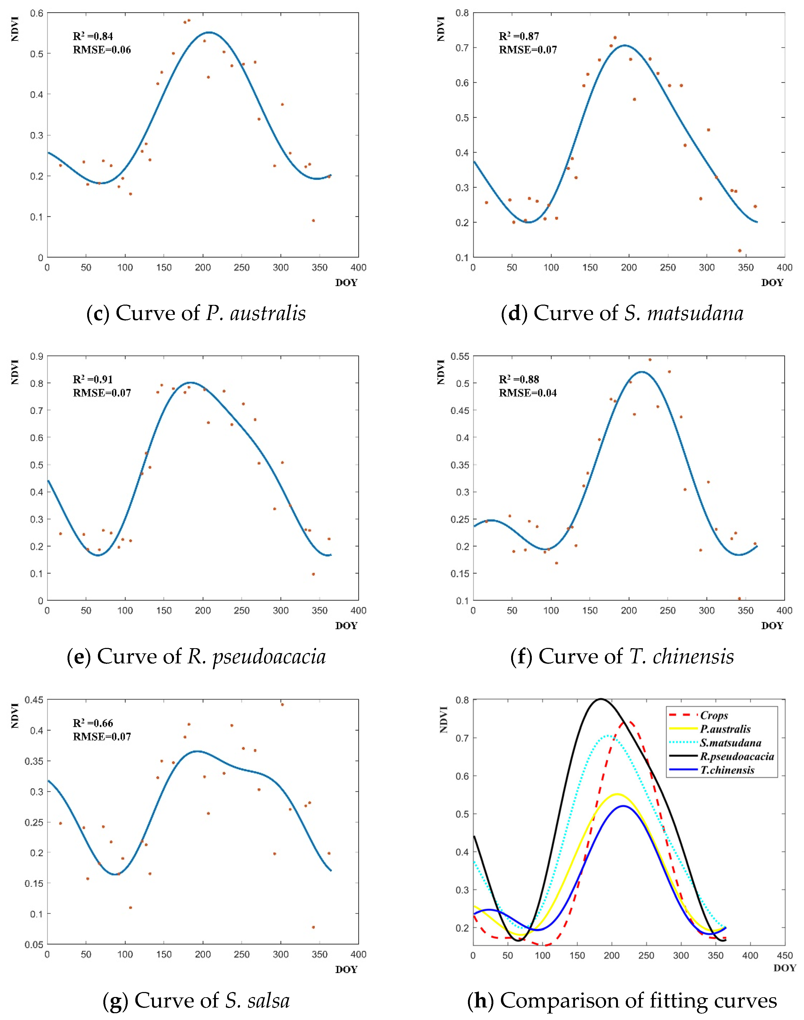
In this section, the RF-PDTS and KNN-TWDTW methods, which were successfully applied in the field of vegetation classification with time series remote sensing data [25,32,33,34] and also performed well in this research, are selected for comparing. The RF-PDTS selects the key phenological phases to classify by analyzing the vegetation growth curve, while the TWDTW and MDDTW both classify by calculating the distance of vegetation growth curve. Therefore, different vegetation growth curves are shown in Figure 12a–g, and confusion matrices from different methods are shown in Table 3 (SA = S. alterniflora, PA = P. australis, SM = S. matsudana, RP = R. pseudoacacia, TC = T. chinensis, SS = S. salsa.). The purpose is to discuss the applicability and deficiencies of different methods by analyzing the growth curves of different vegetation and the misclassification of vegetation.
As shown in Figure 12, the curves of S. alterniflora (b) and S. salsa (g) are obviously different from the others. This is the reason why all classification methods have less misclassification of S. alterniflora and S. salsa in the confusion matrix. Therefore, only the other five types of vegetation are considered in the follow-up comparison. The growth curve comparison is shown in Figure 12h, which clearly shows the differences between the different curves.
In order to describe the misclassification of different vegetation from confusion matrix, the following Equation (16) is used to simply quantify the degree of confusion between the two vegetations:
M ( A , B ) = M B , A + M A , B T A + T B × 100 %
where M ( A , B ) represent the possibility of misclassification between vegetation A and vegetation B, M B , A represents the amount of vegetation A that was misclassified into B, and T A represents the amunt of vegetation A. The same definition applies to M A , B and T B .
For example, M C r o p ,   T C represents the misclassification between Crop and T. chinensis. The higher the value, the greater the possibility of misclassification between the two vegetations. Figure 13 shows the misclassification of different types of vegetation with different methods.
In the RF-PDTS method, P. australis and T. chinensis are the most likely to be misclassified. From Figure 12h, it can be seen that their growth curves (yellow and dark blue curves) are the closest, and the time when the maximum NDVI value occurs of those are both around 210 days. After reaching the maximum value, it almost keeps the same trend and drops to the minimum value. At the same time, the possibility of misclassification between Crop and R. pseudoacacia is the smallest in this method. The reason for this can also be found in Figure 12h. The two vegetations have the largest difference in growth and withering time. In other words, the phenological difference between Crop and R. pseudoacacia is large. Although the overall accuracy of KNN-TWDTW is better than that of the RF-PDTS method, the results in Figure 13 show that the possibility of misclassification in the classification of part of the vegetation is greater than that of the RF-PDTS method, such as P. australis and S. matsudana classification. This is mainly because the TWDTW method expresses its similarity by calculating the distance of the curve as a whole. In the classification of P. australis, S. matsudana, and T. chinensis, this method may consider P. australis (yellow) and S. matsudana (light blue) curves as being more similar in overall shape compared to P. australis and T. chinensis. Nevertheless, the TWDTW method has fully proved its role in the field of time series classification, especially for vegetation with similar phenological time. As for the KNN-MDDTW, it has achieved good results in almost all vegetation.
The difference in phenology is the basis for the RF-PDTS based on time series remote sensing images. The greater the phenological difference of vegetation, the better the classification effect. The vegetation of the YRD wetland is complex, and the growth cycles of different vegetation are similar, which lead to more errors in classification results. The TWDTW method is an improvement based on DTW, relying on time series curves for classification. The TWDTW algorithm works by comparing the similarity between two time-series and finds their optimal alignment, resulting in dissimilarity measures. The time series curve of typical vegetation in the YRD wetland has a high degree of similarity, as shown in Figure 12. Therefore, it has a poor effect on the classification of some vegetation. Compared with RF-PDTS and TWDTW, the KNN-MDDTW has achieved better results, whether it is vegetation with similar phenological time or similar curve shape. The use of a single vegetation index has limited effect on the classification of complex wetland vegetation; however, the KNN-MDDTW shows the effectiveness of using multi-dimensional features for time series classification. This method can calculate reasonable similarity distance from different multi-dimensional features, which meets the needs of classification. But it needs to be pointed out that although the method has achieved good accuracy, its computational cost is also too large to ignore. At the same time, how to select effective features and the importance of different features still needs further research.

4.2. Influence of Parameters on MDDTW Performance

For the classification based on MDDTW, the learning efficiency of M depends on the number of samples. Therefore, it is important to compare the efficiency and accuracy under different sample numbers. The results are shown in Figure 14. It should be pointed out that the experiment was carried out by randomly selecting sample points to calculate time and accuracy, and the result is the average of multiple experiments, which avoid the uncertainty caused by selecting sample points at different positions.
The number of samples has a significant relationship with the accuracy of the final result and the required time. With the increase of the number of samples, the accuracy and kappa both increase, but the time consumption also increases, as shown in Figure 14a. The classification accuracy and kappa coefficient change little with the increase of the number of samples when the number of samples reaches 900. The accuracy has exceeded 90% and kappa was more than 0.9 when the number of samples reaches 1000, as shown in Figure 14b. In the experiment, 1000 samples were chosen for MDDTW classification.

5. Conclusions

The composition and distribution information of wetland vegetation plays a significant role in protecting the wetland ecological environment and formulating effective wetland management plans. In this study, we extracted multiple vegetation indexes based on Sentinel-2 data and studied the multi-dimensional feature time series classification method. The results show that the classification method based on multi-dimensional features has significant advantages in wetland vegetation classification. The overall classification accuracy based on KNN-MDDTW is more than 90% and kappa is more than 0.9, which is better than comparison methods.
The traditional remote sensing time series classification based on DTW has been extended to multi-dimensional feature time series in order to fully utilize spectral information in the current research. This method calculated the similarity distance of multi-dimensional feature time series and effectively improved the accuracy of wetland vegetation classification in the Yellow River Delta, and it is expected to play an important role in the annual dynamic monitoring of wetland vegetation. However, only four indexes (including NDVI, RVI, EVI, and DVI) were selected to construct the multi-dimensional feature time series in the current research. The impact of different index features on classification and the subsequent addition of other features to construct more time series dimensions for classification will be focused on in future research.

Author Contributions

H.L. designed the study, processed the data, and wrote the manuscript draft. H.L., J.W., M.X., S.L. and H.S. revised the manuscript. All authors have read and agreed to the published version of the manuscript.

Funding

Funding: This research was funded by the National Natural Science Foundation of China, grant number 41776182, 62071492.

Data Availability Statement

The satellite remote sensing data used in the research can be downloaded from the European Space Agency (https://scihub.copernicus.eu/dhus/#/home, accessed on 26 November 2021).

Acknowledgments

We gratefully appreciate the editor and anonymous reviewers for their efforts and constructive comments, which have greatly improved the technical quality and presentation of this study.

Conflicts of Interest

The authors declare no conflict of interest.

Appendix A

There are many abbreviations in this study. In order to facilitate reading and understanding, all abbreviations and corresponding explanations are summarized in the Table A1.
Table A1. Acronym List.
AcronymMeaning
YRDYellow River Delta
DTWDynamic Time Warping
MDDTWMahalanobis Distance-based Dynamic Time Warping
KNNK-Nearest Neighbors
NDVINormalized Difference Vegetation Index
EVIEnhanced Vegetation Index
RF-PDTSRandom Forest based on pixel-differential time series
RF-MultitemporalRandom Forest based on multitemporal
TWDTWTime-Weighted Dynamic Time Warping
EDDTWDTW based on Euclidean distance
DVIDifference Vegetation Index
RVIRatio Vegetation Index

References

  1. Hempattarasuwan, N.; Christakos, G.; Wu, J. Changes of Wiang Nong Lom and Nong Luang wetlands in Chiang Saen Valley (Chiang Rai Province, Thailand) during the period 1988–2017. IEEE J. Sel. Top. Appl. Earth Obs. Remote Sens. 2019, 12, 4224–4238. [Google Scholar] [CrossRef]
  2. Wang, Y.; Feng, J.; Lin, Q.; Lyu, X.; Wang, X.; Wang, G. Effects of crude oil contamination on soil physical and chemical properties in Momoge wetland of China. Chin. Geogr. Sci. 2013, 23, 708–715. [Google Scholar] [CrossRef]
  3. Kumar, T.; Mandal, A.; Dutta, D.; Nagaraja, R.; Dadhwal, V.K. Discrimination and classification of mangrove forests using EO-1 Hyperion data: A case study of Indian Sundarbans. Geocarto Int. 2019, 34, 415–442. [Google Scholar] [CrossRef]
  4. Feddema, J.J.; Oleson, K.W.; Bonan, G.B.; Mearns, L.O.; Buja, L.E.; Meehl, G.A.; Washington, W.M. The importance of land-cover change in simulating future climates. Science 2005, 310, 1674–1678. [Google Scholar] [CrossRef] [Green Version]
  5. Gallant, A.L. The challenges of remote monitoring of wetlands. Remote Sens. 2015, 7, 10938–10950. [Google Scholar] [CrossRef] [Green Version]
  6. Zhao, G.; Ye, S.; Gao, M.; Ding, X.; Yuan, H.; Wang, J. Change analysis on eco-environment of the estuary wetland reserve area of Yellow River Delta based on RS and GIS. In Proceedings of the 19th International Conference on Geoinformatics, Shanghai, China, 24–26 June 2011; pp. 1–4. [Google Scholar]
  7. Cabezas, J.; Galleguillos, M.; Perez-Quezada, J.F. Predicting vascular plant richness in a heterogeneous wetland using spectral and textural features and a random forest algorithm. IEEE Geosci. Remote Sens. Lett. 2016, 13, 646–650. [Google Scholar] [CrossRef]
  8. Dang, A.T.N.; Kumar, L.; Reid, M.; Nguyen, H. Remote sensing approach for monitoring coastal wetland in the Mekong Delta, Vietnam: Change trends and their driving forces. Remote Sens. 2021, 13, 3359. [Google Scholar] [CrossRef]
  9. Desclee, B.; Simonetti, D.; Mayaux, P.; Achard, F. Multi-sensor monitoring system for forest cover change assessment in central Africa. IEEE J. Sel. Top. Appl. Earth Obs. Remote Sens. 2013, 6, 110–120. [Google Scholar] [CrossRef]
  10. Liu, T.; Zhang, X.; Gu, Y. Unsupervised cross-temporal classification of hyperspectral images with multiple geodesic flow kernel learning. IEEE Trans. Geosci. Remote Sens. 2019, 57, 9688–9701. [Google Scholar] [CrossRef]
  11. Soares, A.; Korting, T.; Fonseca, L.; Bendini, H. Simple nonlinear iterative temporal clustering. IEEE Trans. Geosci. Remote Sens. 2021, 59, 7669–7679. [Google Scholar] [CrossRef]
  12. Montgomery, J.; Mahoney, C.; Brisco, B.; Boychuk, L.; Cobbaert, D.; Hopkinson, C. Remote sensing of wetlands in the prairie pothole region of North America. Remote Sens. 2021, 13, 3878. [Google Scholar] [CrossRef]
  13. Leonairo Pencue-Fierro, E.; Solano-Correa, Y.T.; Carlos Corrales-Munoz, J.; Figueroa-Casas, A. A semi-supervised hybrid approach for multitemporal multi-region multisensor Landsat data classification. IEEE J. Sel. Top. Appl. Earth Obs. Remote Sens. 2016, 9, 5424–5435. [Google Scholar] [CrossRef]
  14. Li, X.; Shen, H.; Zhang, L.; Zhang, H.; Yuan, Q.; Yang, G. Recovering quantitative remote sensing products contaminated by thick clouds and shadows using multitemporal dictionary learning. IEEE Trans. Geosci. Remote Sens. 2014, 52, 7086–7098. [Google Scholar]
  15. Gao, J.; Yi, Y.; Wei, T.; Zhang, H. Sentinel-2 cloud removal considering ground changes by fusing multitemporal SAR and optical images. Remote Sens. 2021, 13, 3998. [Google Scholar] [CrossRef]
  16. Melaas, E.K.; Friedl, M.A.; Zhu, Z. Detecting interannual variation in deciduous broadleaf forest phenology using Landsat TM/ETM plus data. Remote Sens. Environ. 2013, 132, 176–185. [Google Scholar] [CrossRef]
  17. Gomez, C.; White, J.C.; Wulder, M.A. Optical remotely sensed time series data for land cover classification: A review. ISPRS J. Photogramm. Remote Sens. 2016, 116, 55–72. [Google Scholar] [CrossRef] [Green Version]
  18. Wozniak, E.; Kofman, W.; Aleksandrowicz, S.; Rybicki, M.; Lewinski, S. Multi-temporal indices derived from time series of Sentinel-1 images as a phenological description of plants growing for crop classification. In Proceedings of the 10th International Workshop on the Analysis of Multitemporal Remote Sensing Images (MULTITEMP), Shanghai, China, 5–7 August 2019; pp. 1–4. [Google Scholar]
  19. Evans, J.P.; Geerken, R. Classifying rangeland vegetation type and coverage using a Fourier component based similarity measure. Remote Sens. Environ. 2006, 105, 1–8. [Google Scholar] [CrossRef]
  20. Brooks, E.B.; Thomas, V.A.; Wynne, R.H.; Coulston, J.W. Fitting the multitemporal curve: A Fourier series approach to the missing data problem in remote sensing analysis. IEEE Trans. Geosci. Remote Sens. 2012, 50, 3340–3353. [Google Scholar] [CrossRef] [Green Version]
  21. Du, J.; Shi, J.; Liu, Q.; Jiang, L. Refinement of microwave vegetation index using Fourier analysis for monitoring vegetation dynamics. IEEE Geosci. Remote Sens. Lett. 2013, 10, 1205–1208. [Google Scholar] [CrossRef]
  22. Chen, J.; Rao, Y.; Shen, M.; Wang, C.; Zhou, Y.; Ma, L.; Tang, Y.; Yang, X. A simple method for detecting phenological change from time series of vegetation index. IEEE Trans. Geosci. Remote Sens. 2016, 54, 3436–3449. [Google Scholar] [CrossRef]
  23. Zhong, L.; Hu, L.; Yu, L.; Gong, P.; Biging, G.S. Automated mapping of soybean and corn using phenology. ISPRS J. Photogramm. Remote Sens. 2016, 119, 151–164. [Google Scholar] [CrossRef] [Green Version]
  24. Granero-Belinchon, C.; Adeline, K.; Lemonsu, A.; Briottet, X. Phenological dynamics characterization of alignment trees with Sentinel-2 imagery: A vegetation indices time series reconstruction methodology adapted to urban areas. Remote Sens. 2020, 12, 639. [Google Scholar] [CrossRef] [Green Version]
  25. Sun, C.; Li, J.; Liu, Y.; Liu, Y.; Liu, R. Plant species classification in salt marshes using phenological parameters derived from Sentinel-2 pixel-differential time-series. Remote Sens. Environ. 2021, 256, 112320. [Google Scholar] [CrossRef]
  26. Zurita-Milla, R.; Van Gijsel, J.A.E.; Hamm, N.A.; Augustijn, P.W.M.; Vrieling, A. Exploring spatiotemporal phenological patterns and trajectories using self-organizing maps. IEEE Trans. Geosci. Remote Sens. 2013, 51, 1914–1921. [Google Scholar] [CrossRef]
  27. Lee, B.; Kim, E.; Lim, J.; Seo, B.; Chung, J. Detecting vegetation phenology in various forest types using long-term MODIS vegetation indices. In Proceedings of the 2018 IEEE International Geoscience and Remote Sensing Symposium (IGARSS), Valencia, Spain, 23–27 July 2018; pp. 5243–5246. [Google Scholar]
  28. Ghaderpour, E.; Vujadinovic, T. Change detection within remotely sensed satellite image time series via spectral analysis. Remote Sens. 2020, 12, 4001. [Google Scholar] [CrossRef]
  29. Petitjean, F.; Inglada, J.; Gancarski, P. Satellite image time series analysis under time warping. IEEE Trans. Geosci. Remote Sens. 2012, 50, 3081–3095. [Google Scholar] [CrossRef]
  30. Jiang, Y.; Qi, Y.; Wang, W.K.; Bent, B.; Avram, R.; Olgin, J.; Dunn, J. EventDTW: An improved dynamic time warping algorithm for aligning biomedical signals of nonuniform sampling frequencies. Sensors 2020, 20, 2700. [Google Scholar] [CrossRef]
  31. Guan, X.; Huang, C.; Liu, G.; Meng, X.; Liu, Q. Mapping rice cropping systems in Vietnam using an NDVI-based time-series similarity measurement based on DTW distance. Remote Sens. 2016, 8, 19. [Google Scholar] [CrossRef] [Green Version]
  32. Maus, V.; Camara, G.; Cartaxo, R.; Sanchez, A.; Ramos, F.M.; de Queiroz, G.R. A time-weighted dynamic time warping method for land-use and land-cover mapping. IEEE J. Sel. Top. Appl. Earth Obs. Remote Sens. 2016, 9, 3729–3739. [Google Scholar] [CrossRef]
  33. Belgiu, M.; Csillik, O. Sentinel-2 cropland mapping using pixel-based and object-based time-weighted dynamic time warping analysis. Remote Sens. Environ. 2018, 204, 509–523. [Google Scholar] [CrossRef]
  34. Zhao, F.; Yang, G.; Yang, X.; Cen, H.; Zhu, Y.; Han, S.; Yang, H.; He, Y.; Zhao, C. Determination of key phenological phases of winter wheat based on the time-weighted dynamic time warping algorithm and MODIS time-series data. Remote Sens. 2021, 13, 1836. [Google Scholar] [CrossRef]
  35. Hao, P.; Wang, L.; Zhan, Y.; Niu, Z.; Wu, M. Using historical NDVI time series to classify crops at 30 m spatial resolution: A case in Southeast Kansas. In Proceedings of the 2016 IEEE International Geoscience and Remote Sensing Symposium (IGARSS), Beijing, China, 10–15 July 2016; pp. 6316–6319. [Google Scholar]
  36. Huang, Y.; Liu, X.; Li, X.; Yan, Y.; Ou, J. Comparing the effects of temporal features derived from synthetic time-series NDVI on fine land cover classification. IEEE J. Sel. Top. Appl. Earth Obs. Remote Sens. 2018, 11, 4618–4629. [Google Scholar] [CrossRef]
  37. Csillik, O.; Belgiu, M.; Asner, G.P.; Kelly, M. Object-based time-constrained dynamic time warping classification of crops using Sentinel-2. Remote Sens. 2019, 11, 1257. [Google Scholar] [CrossRef] [Green Version]
  38. Lewandowski, M.; Makris, D.; Velastin, S.A.; Nebel, J.C. Structural laplacian eigenmaps for modeling sets of multivariate sequences. IEEE Trans. Cybern. 2014, 44, 936–949. [Google Scholar] [CrossRef] [PubMed]
  39. Gupta, A.; Gupta, H.P.; Biswas, B.; Dutta, T. Approaches and applications of early classification of time series: A review. IEEE Trans. Artif. Intell. 2020, 1, 47–61. [Google Scholar] [CrossRef]
  40. Weng, X.; Shen, J. Classification of multivariate time series using two-dimensional singular value decomposition. Knowl.-Based Syst. 2008, 21, 535–539. [Google Scholar] [CrossRef]
  41. Liu, C.; Tao, R.; Li, W.; Zhang, M.; Sun, W.; Du, Q. Joint classification of hyperspectral and multispectral images for mapping coastal wetlands. IEEE J. Sel. Top. Appl. Earth Obs. Remote Sens. 2021, 14, 982–996. [Google Scholar] [CrossRef]
  42. Louis, J.; Pflug, B.; Main-Knorn, M.; Debaecker, V.; Mueller-Wilm, U.; Iannone, R.Q.; Cadau, E.G.; Boccia, V.; Gascon, F. Sentinel-2 global surface reflectance level-2a product generated with Sen2cor. In Proceedings of the 2019 IEEE International Geoscience and Remote Sensing Symposium (IGARSS), Yokohama, Japan, 28 July–2 August 2019; pp. 8522–8525. [Google Scholar]
  43. Qiu, S.; Zhu, Z.; He, B. Fmask 4.0: Improved cloud and cloud shadow detection in Landsats 4–8 and Sentinel-2 imagery. Remote Sens. Environ. 2019, 231, 111205. [Google Scholar] [CrossRef]
  44. Jordan, C.F. Derivation of leaf-area index from quality of light on the forest floor. Ecology 1969, 50, 663–666. [Google Scholar] [CrossRef]
  45. Liu, H.Q.; Huete, A. A feedback based modification of the NDVI to minimize canopy background and atmospheric noise. IEEE Trans. Geosci. Remote Sens. 1995, 33, 457–465. [Google Scholar] [CrossRef]
  46. Zhu, Y.; Yao, X.; Tian, Y.; Liu, X.; Cao, W. Analysis of common canopy vegetation indices for indicating leaf nitrogen accumulations in wheat and rice. Int. J. Appl. Earth Obs. Geoinf. 2008, 10, 1–10. [Google Scholar] [CrossRef]
  47. Qian, L.; Zhang-qin, H.; Yi-bin, H.; Rui, C. Utterance verification on DTW based speech recognition using likelihood. In Proceedings of the 2010 International Conference on Computer Application and System Modeling (ICCASM 2010), Taiyuan, China, 22–24 October 2010; Volume 2, pp. 427–431. [Google Scholar]
  48. Jambhale, S.S.; Khaparde, A. Gesture recognition using DTW & piecewise DTW. In Proceedings of the 2014 21st International Conference on Electronics and Communication Systems (ICECS 2014), Marseille, France, 7–10 December 2014; pp. 1–5. [Google Scholar]
  49. Lampert, T.; Lafabregue, B.; Gançarski, P. Constrained distance-based clustering for satellite image time-series. IEEE J. Sel. Top. Appl. Earth Obs. Remote Sens. 2019, 12, 4606–4621. [Google Scholar] [CrossRef]
  50. Wang, X.; Jiang, M.; Chen, S.; Yang, C.; Jing, W.; Guo, Z. A hybrid time series matching algorithm based on feature-points and DTW. In Proceedings of the 2016 9th International Symposium on Computational Intelligence and Design (ISCID 2016), Hangzhou, China, 10–11 December 2016; Volume 2, pp. 171–175. [Google Scholar]
  51. Zhong, Y.; Lin, X.; Zhang, L. A support vector conditional random fields classifier with a Mahalanobis distance boundary constraint for high spatial resolution remote sensing imagery. IEEE J. Sel. Top. Appl. Earth Obs. Remote Sens. 2014, 7, 1314–1330. [Google Scholar] [CrossRef]
  52. Shen, C.; Kim, J.; Wang, L. Scalable large-margin Mahalanobis distance metric learning. IEEE Trans. Neural Netw. 2010, 21, 1524–1530. [Google Scholar] [CrossRef] [Green Version]
  53. Mei, J.; Liu, M.; Karimi, H.R.; Gao, H. LogDet divergence-based metric learning with triplet constraints and its applications. IEEE Trans. Image Process. 2014, 23, 4920–4931. [Google Scholar] [CrossRef] [PubMed]
  54. Mei, J.; Liu, M.; Wang, Y.F.; Gao, H. Learning a Mahalanobis distance-based dynamic time warping measure for multivariate time series classification. IEEE Trans. Cybern. 2016, 46, 1363–1374. [Google Scholar] [CrossRef] [PubMed]
  55. Davis, J.V.; Kulis, B.; Jain, P.; Sra, S.; Dhillon, I.S. Information-theoretic metric learning. Machine Learning. In Proceedings of the Twenty-Fourth International Conference (ICML 2007), Corvallis, OR, USA, 20–24 June 2007; pp. 209–216. [Google Scholar]
  56. Jain, P.; Kulis, B.; Dhillon, I.S.; Grauman, K. Online metric learning and fast similarity search. Advances in Neural Information Processing Systems 21. In Proceedings of the Twenty-Second Annual Conference on Neural Information Processing Systems, Vancouver, BC, Canada, 8–11 December 2008; pp. 761–768. [Google Scholar]
  57. Bernhard, S.; John, P.; Thomas, H. Differential Entropic Clustering of Multivariate Gaussians. In Advances in Neural Information Processing Systems 19: Proceedings of the 2006 Conference; MIT Press: Cambridge, MA, USA, 2007; pp. 337–344. [Google Scholar]
  58. Orsenigo, C.; Vercellis, C. Combining discrete SVM and fixed cardinality warping distances for multivariate time series classification. Pattern Recogn. 2010, 43, 3787–3794. [Google Scholar] [CrossRef]
  59. Gravano, L.; Paparrizos, J. K-shape: Efficient and accurate clustering of time series. In Proceedings of the 2015 ACM SIGMOD International Conference on Management of Data, Melbourne, Victoria, Australia, 27 May 2015; Volume 45, pp. 69–76. [Google Scholar]
  60. Qu, C.; Li, P. Winter wheat mapping from Landsat NDVI time series data using time-weighted dynamic time warping and phenological rules. In Proceedings of the 2020 IEEE International Geoscience and Remote Sensing Symposium (IGARSS), Waikoloa, HI, USA, 26 September–2 October 2020; pp. 4183–4186. [Google Scholar]
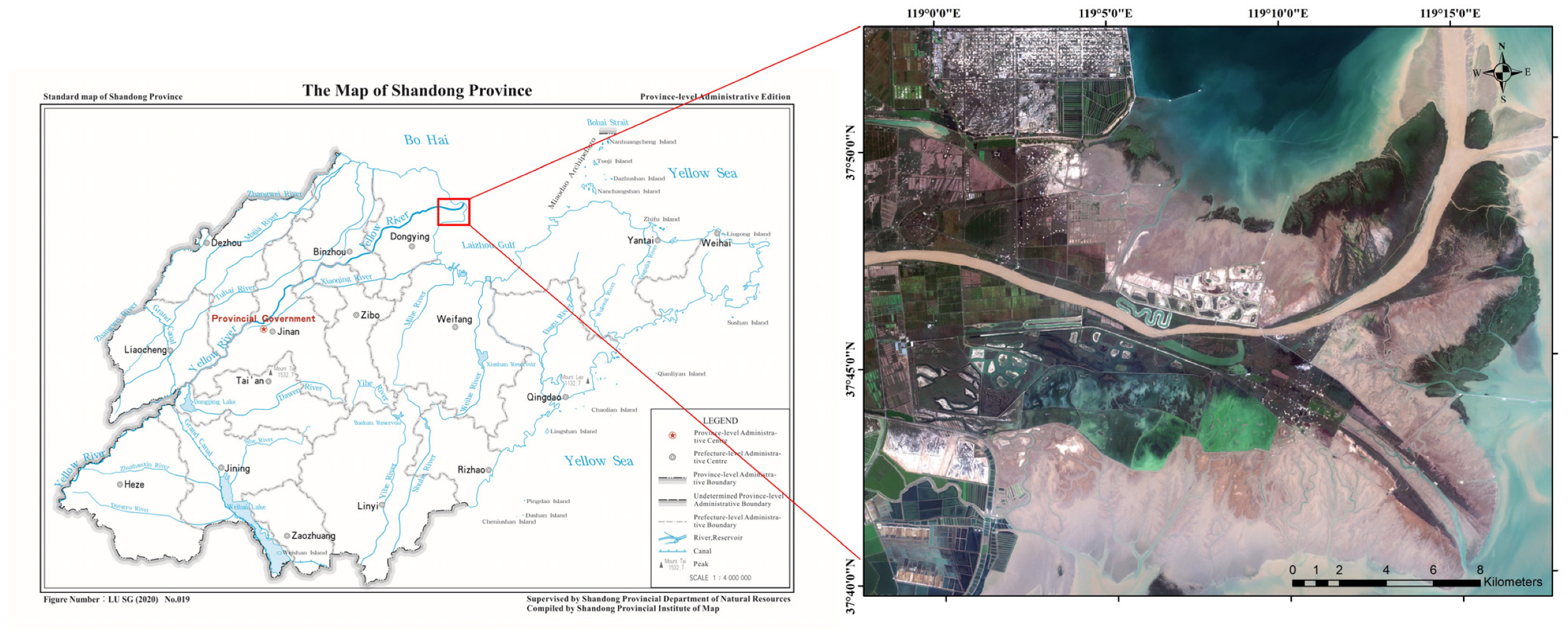
Figure 1. Location of study area in Shandong Province of China. The image to the right is a true color composite (red, green, blue bands) from Sentinel-2.
Remotesensing 14 00501 g001
Figure 2. The distribution of field survey points overlaid on the Sentinel-2 MSI false-color images (R: 8, G: 4, B: 3). The image to the right is the photo of different vegetation types, including (a) P. australis, (b) S. alterniflora, (c) T. chinensis, (d) R. pseudoacacia, (e) S. salsa, (f) S. matsudana.
Remotesensing 14 00501 g002
Figure 3. The distribution of verification points.
Remotesensing 14 00501 g003
Figure 4. Classification of vegetation, tidal flat, and water.
Remotesensing 14 00501 g004
Figure 5. The workflow of KNN-MDDTW classification.
Remotesensing 14 00501 g005
Figure 6. The optimal warping path between time series X and Y (red squares).
Remotesensing 14 00501 g006
Figure 7. Images for Multi-season Random Forest classification. (a) 1 February 2019. (b) 2 May 2019. (c) 1 July 2019. (d) 8 November 2019.
Remotesensing 14 00501 g007
Figure 8. Parameter settings of TWDTW. (a) OA/kappa-β (α = 0.1). (b) OA/kappa-α (β = 45).
Remotesensing 14 00501 g008
Figure 9. Classification map of different methods: (a) RF-Multitemporal images, (b) RF-PDTS, (c) RF-TWDTW, (d) KNN-TWDTW, (e) RF-EDDTW, (f) KNN-EDDTW, (g) RF-MDDTW, (h) KNN-MDDTW.
Remotesensing 14 00501 g009aRemotesensing 14 00501 g009b
Figure 10. Producer accuracy of different classification methods.
Remotesensing 14 00501 g010
Figure 11. User accuracy of different classification methods.
Remotesensing 14 00501 g011
Figure 12. Fitting curve of wetland vegetation.
Remotesensing 14 00501 g012aRemotesensing 14 00501 g012b
Figure 13. Misclassification of different vegetation with different methods.
Remotesensing 14 00501 g013
Figure 14. The relationship between number of samples, time-consumption, and classification accuracy. (a) Time–Number of samples. (b) OA/kappa–Number of samples.
Remotesensing 14 00501 g014
Table 1. Satellite image dates.
Satellite NameSentinel-2 Sensing Date in 2019
Sentinel-2A02/2103/1303/2304/0205/0205/1205/2206/1107/01
07/2109/0909/2910/1910/2911/0811/2812/0812/28
Sentinel-2B01/1702/1603/0804/0704/1705/0705/2706/2607/26
08/1508/2509/2412/03
Table 2. Accuracy of different classification methods.
Classification TypeOA (%)Kappa
RF-Multitemporal80.630.77
RF-PDTS88.300.85
RF-TWDTW78.580.75
KNN-TWDTW91.250.89
RF-EDDTW70.950.66
KNN-EDDTW86.500.83
RF-MDDTW82.390.79
KNN-MDDTW94.560.93
Table 3. Confusion matrix of the wetland vegetation classification.
CropsSAPASMRPTCSSPA
Method: RF-PDTS, Overall accuracy = 88.30%, kappa = 0.85
Crops5240183211093.91%
SA012403010099.68%
PA40010227515100081.63%
SM39676235190062.67%
RP005111160069.05%
TC65120100222061.12%
SS0000001188100%
UA86.04%99.12%79.22%72.53%75.82%66.67%100%
Method: KNN-TWDTW, Overall accuracy = 91.25%, kappa = 0.89
Crops530029334093.15%
SA2124211200098.81%
PA345109767549087.27%
SM121106251133065.03%
RP40111320095.65%
TC1836500274076.11%
SS305003118899.08%
UA87.89%99.28%83.49%77.47%86.27%82.28%100.00%
Method: KNN-MDDTW, Overall accuracy = 94.56%, kappa = 0.93
Crops565118010096.58%
SA012245101099.43%
PA2423120966919089.56%
SM404625521082.79%
RP10021400097.90%
TC913501304086.86%
SS021008118899.08%
UA93.70%97.84%92.01%78.70%91.50%91.29%100.00%
Publisher’s Note: MDPI stays neutral with regard to jurisdictional claims in published maps and institutional affiliations.