Abstract
Atmospheric corrections introduce uncertainties in bottom-of-atmosphere Ocean Colour (OC) products. In this paper, we analyse the uncertainty budget of the SeaDAS atmospheric correction algorithm. A metrological approach is followed, where each of the error sources are identified in an uncertainty tree diagram and briefly discussed. Atmospheric correction algorithms depend on ancillary variables (such as meteorological properties and column densities of gases), yet the uncertainties in these variables were not studied previously in detail. To analyse these uncertainties for the first time, the spread in the ERA5 ensemble is used as an estimate for the uncertainty in the ancillary data, which is then propagated to uncertainties in remote sensing reflectances using a Monte Carlo approach and the SeaDAS atmospheric correction algorithm. In an example data set, wind speed and relative humidity are found to be the main contributors (among the ancillary parameters) to the remote sensing reflectance uncertainties.
1. Introduction
Ocean colour remote sensing opens a window onto ocean biology through the calculation of chlorophyll-a concentration from radiometric remote sensing reflectance (normalised water-leaving radiances) measurements. To obtain the water-leaving radiances, the top-of-atmosphere (TOA) radiances measured by the satellite instrument have to be corrected for atmospheric (aerosols and Rayleigh scattering) and surface (glint and foam) contributions.
Just like any other physical measurement, Ocean Colour (OC) products require estimates of their uncertainties to be meaningful. Without, there is no way to assess their quality or understand how far the true value may be from the measured value. Radiometric uncertainty (at k = 2) lower than 5% in the blue and green spectral regions along with 0.5% decadal stability was listed by the Global Climate Observing System (GCOS) as requirements for water-leaving radiance as an Essential Climate Variable [1]. There are various sources of uncertainty in OC products. Two of the main contributions are the radiometric properties and stability of the sensor and the uncertainties in the atmospheric correction, the process that determines the water-leaving radiance (or reflectance) from the TOA radiances [2]. The uncertainty of the atmospheric correction depends on the algorithm used as well as on the distribution of gases and aerosols in the atmosphere.
In clear sky conditions, the processes affecting the atmospheric correction are gaseous absorption, molecular scattering, aerosol scattering and absorption, and water surface (Fresnel) reflection. Gaseous absorption is easy to handle when the satellite sensors observe in atmospheric windows (the usual case) where molecular scattering can be computed accurately. The influence of scattering by aerosols and Fresnel reflection (waves, whitecaps and surface perturbations due to wind) are both highly variable in space and time and are more difficult to correct.
The standard approach for atmospheric correction, first suggested by [3], consists of first estimating the aerosol/surface reflectance in the red and near-infrared where the water body can be considered as totally absorbing (i.e., black), and then extrapolating the aerosol/surface reflectance to the other wavelengths. In many cases (e.g., coastal waters) the water reflectance in the red and near-infrared is not completely zero, and corrections were proposed to improve the algorithms in these cases, e.g., [4,5].
There are many software packages (e.g., the Sea-viewing Wide Field-of-view Sensor (SeaWiFS) Data Analysis System, SeaDAS, developed by NASA) which successfully implement these standard approach algorithms and use reanalysis datasets for obtaining the ancillary parameters necessary in the atmospheric correction (mostly information about meteorological conditions and ozone concentration). Reanalysis datasets such as the one produced by National Centers for Environmental Prediction (NCEP) or by the European Centre for Medium-Range Weather Forecast (ECMWF) are created using the data assimilation schemes of numerical weather prediction (NWP) models which assimilate observations over the entire reanalysis period. The R2 NCEP reanalysis dataset is presented in [6] and the ECMWF Reanalysis 5th Generation (ERA5) in [7]. For completeness, there also exist other approaches for atmospheric correction, such as algorithms that simultaneously fit the surface reflectances and key properties of the atmosphere (e.g., aerosol type and optical depth). These pose the atmospheric correction as an inverse problem, which can be solved deterministically e.g., [8,9] or using a Bayesian approach e.g., [10].
In this paper, we use a metrological approach established in the Fidelity and uncertainty in climate data records from Earth Observations (FIDUCEO) project [11] to study the uncertainty in the atmospheric correction using the SeaDAS “l2gen” algorithm [12,13,14], and apply it to investigate how uncertainties in ancillary data impact the atmospheric correction, a topic that was little addressed so far in the OC community. In Section 2, we detail the TOA SeaWiFS data used in this work and the NCEP and ERA5 reanalysis datasets. In Section 3, we discuss the SeaDAS uncertainty budget, build the uncertainty tree diagram and discuss the uncertainty contributions. In Section 4, the distribution of the global ancillary variables and their uncertainties is presented.
Next, Section 5 explains the uncertainty propagation method. We illustrate this method in Section 6 by showing results obtained by propagating the ancillary data uncertainties to uncertainties on remote sensing reflectance for two example SeaWiFS scenes analysed in this paper. Finally, Section 7 lists the conclusions. In a companion paper to this work (Mélin et al., submit.), we perform a comprehensive analysis of the effects of the ancillary data as well as their uncertainties, spanning the whole globe and all of 2003 using consistent methods.
2. Data Description
To investigate the uncertainties introduced by ancillary variables, we apply the l2gen algorithm to Level-1A (L1A) TOA data from the Sea-Viewing Wide Field-of-View Sensor (SeaWiFS, [15]) using various sets of ancillary data from reanalysis datasets. In this section, we start by describing the L1 and reanalysis data used in this work.
2.1. L1 Data
SeaWiFS was a sensor on the OrbView-2 satellite launched in 1997, and it collected data until 2010. Its main goal was to collect ocean colour measurements at 4 km and 1 km resolution in 8 spectral bands. We study the various uncertainty contributions associated with ancillary data on the pixel level. Only two SeaWiFS scenes were used, yet we note the same methods can be applied to each of the instruments that can be processed by SeaDAS, and for any given scene.
The two scenes were chosen somewhat at random, while discarding scenes with too much cloud cover. We chose one case with significant variability in the OC products, and one case with quite little variation (see also Section 6). The scene with significant variability is off the west coast of Australia, observed on the 7 April 1999. The variability is caused by an algae bloom. For this scene we use the Merged Local Area Coverage (MLAC) SeaWiFS data with spatial resolution of 1.1 km. Our other case is in the Atlantic ocean, north of Suriname, and was observed on the 30 December 2004. Here, we used the Global Area Coverage (GAC) SeaWiFS data with effective resolution of about 4.5 km. In addition to the two scenes that are the focus of this study, we studied some additional scenes to check whether the conclusions made for our two main scenes hold for other cases. Mélin et al. (submit.) perform a systematic study of the effects of the ancillary parameter uncertainties using all SeaWiFS L1A GAC data for the year 2003.
2.2. NCEP Reanalysis Dataset
The SeaDAS ocean colour processing typically uses the Reanalysis 2 (R2) dataset [6] produced by NCEP and the US Department of Energy, together with ozone products from the Total Ozone Mapping Spectrometer (TOMS) [16] instrument. R2 is a reanalysis data set with spatial resolution spanning from 1979 to the present. The dataset provides data for a range of variables every 6 h with a latency of between 2 and 6 weeks. Improvements were made from its predecessor, NCEP Reanalysis, by reducing its coverage to commence alongside the first satellite observations to make the data more consistent throughout the record. For the results in Section 6, the NCEP data were acquired by SeaDAS itself. Additionally, we downloaded data from all of 2002, and investigate the spread in ancillary parameters in Section 4.
2.3. ERA5 Reanalysis Dataset
ECMWF released their latest meteorological reanalysis dataset, ERA5, in 2018. It currently extends from 1979 up to the present. The reanalysis runs one day behind real time and products are available 5 days behind real time. A preliminary dataset is available from 1950 to 1978 [17]. In addition to an hourly high resolution product (31 km horizontal resolution) ERA5 also provides a ten-member ensemble of analyses every three hours for a range of variables at 62 km spatial resolution. The ensemble provides an estimate of the uncertainties in the ERA5 analyses, taking into account uncertainties in the underlying forecast model (used to propagate the analysis state between assimilation cycles) and in the assimilated observations.
ERA5 is a state-of-the-art reanalysis dataset that benefits from many years of developments in model physics, core dynamics and data assimilation [7]. In addition to the high spatial and temporal resolution (for a global reanalysis), it uses the ECMWF Integrated Forecasting System at Cycle 41r2 (the most up-to-date version of the ECMWF model when ERA5 was started in 2016). Each member of the ensemble (except the control) is run with different random perturbations added to the observations. The perturbations of observations are sampled from a zero-mean Gaussian distribution with variance equal to the expected variances of the observation errors. Likewise, the model physical tendencies are perturbed [18] in the short forecasts that link subsequent analysis windows. Perturbations in Sea Surface Temperature (SST) and Sea Ice Concentration (SIC) are taken from the spread within the range of available products [19]. The perturbations applied to the observations, the SST, SIC, and the model imply that the resulting background (i.e., the short-range forecast linking successive analyses) of each member is implicitly perturbed, thus avoiding the need for explicitly perturbing the background fields. This leads to an uncertainty contribution which is correlated over the whole image, and over a few timesteps for each ensemble member. Even though multiple systematic biases are highly likely, the random uncertainties dominate the spread between ensemble members at the pixel-level. However, averaged data (e.g., monthly or global averages) will likely be dominated by correlated uncertainties. The ERA5 data for the times associated with our SeaWiFS scenes, as well as data for all of 2002, were downloaded from the Copernicus Climate Change Service (C3S) Climate Data Store (CDS) [20].
3. SeaDAS Uncertainty Budget
The SeaDAS software package was used by NASA to produce OC products for many years. The package was originally produced by the NASA Ocean Biology Processing Group for the SeaWiFS satellite mission, but is now able to manage multiple missions (e.g., the Moderate Resolution Imaging Spectroradiometer (MODIS), Medium Resolution Imaging Spectrometer (MERIS), Ocean Colour Monitor-2 (OCM2), Ocean Colour and Temperature Scanner (OCTS) and Coastal Zone Colour Scanner (CZCS) among others). Since the software is open source, a metrological analysis of it is possible. This, combined with its widespread use, is why we opted to use SeaDAS in our analysis.
For this study, we are analysing uncertainty contributions using the SeaDAS tool for processing from L1 to L2, “l2gen” version 7.5.1 [14]. This tool reads TOA radiances and applies an atmospheric correction algorithm to determine remote sensing reflectance, , in spectral channels , making use of ancillary meteorological data that describe the atmospheric state during the observation. For a detailed description of the SeaDAS l2gen processing we refer to [12,13,14,21].
3.1. Uncertainty Tree Diagrams
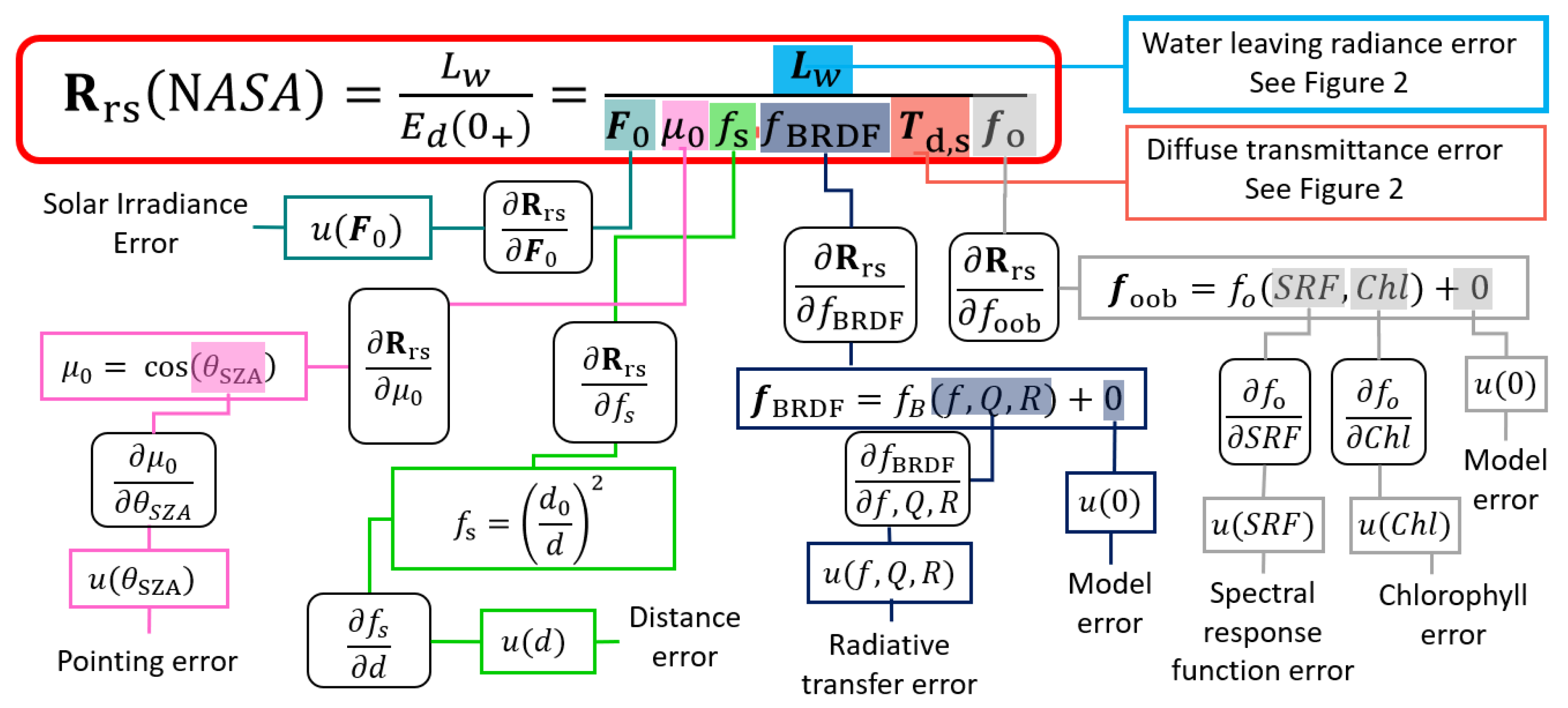
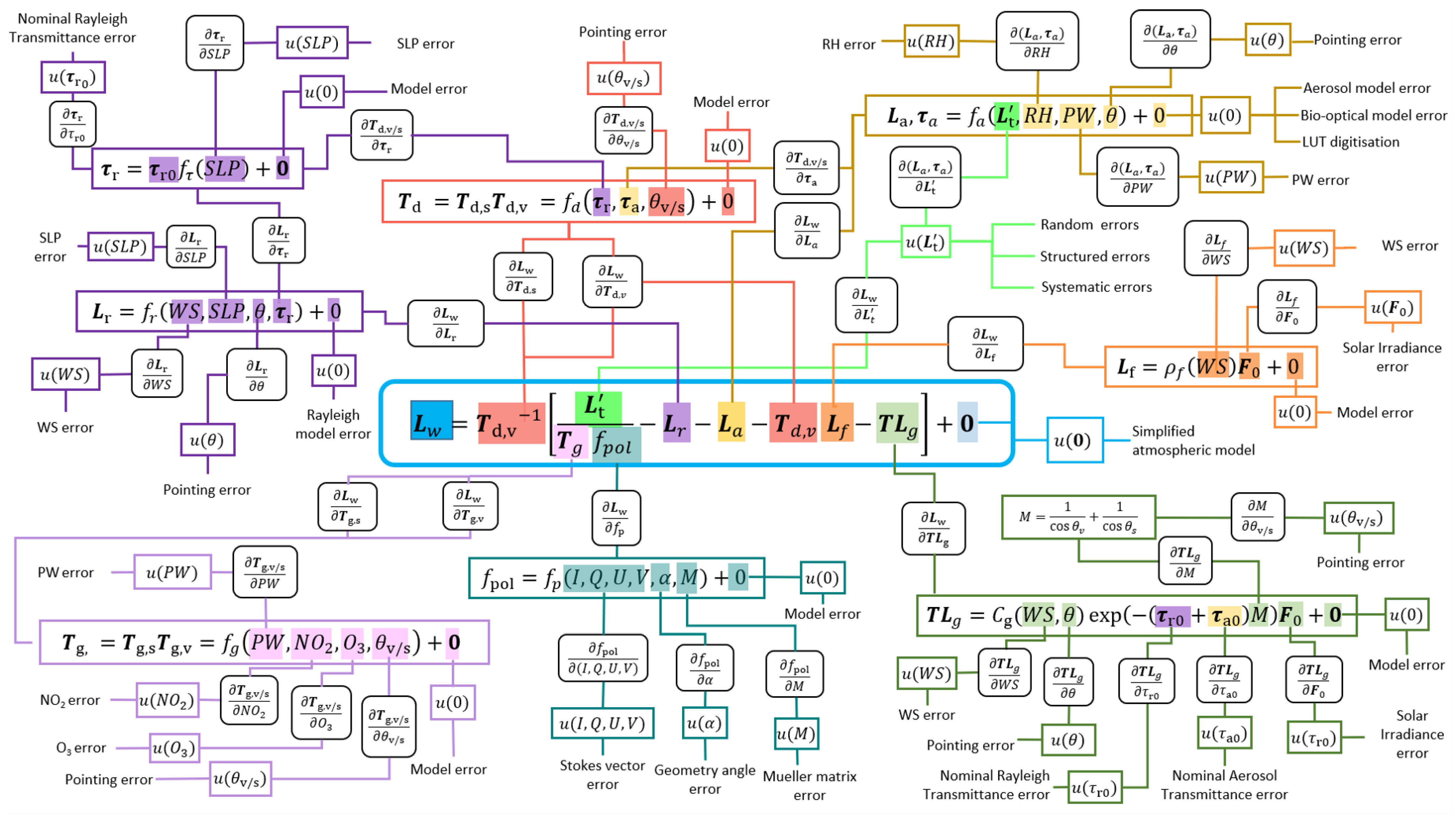
To represent the different uncertainty contributions to the SeaDAS l2gen process, we follow the approach outlined in the FIDUCEO project [11] and produce an uncertainty tree diagram. At the centre of the diagram in Figure 1 is the measurement function for how l2gen calculates the remote sensing reflectances () from the water leaving radiance () obtained after atmospheric correction. From this function branches spread from each input quantity, which may themselves be determined by their own measurement functions. A separate diagram is given in Figure 2 for the calculation of the water-leaving radiances. Each of the sources of uncertainty can be traced back through to its impact on the measurand by the sensitivity coefficients (partial derivatives) on each branch. Finally, the effects which cause each respective uncertainty are connected to the end of each branch. Note that most measurement functions used are not a perfect representation of reality. To account for the difference between the true physical effects and the measurement functions used, a +0 term (a term with an expected value of zero but with positive uncertainty) is included at the end of most measurement functions.
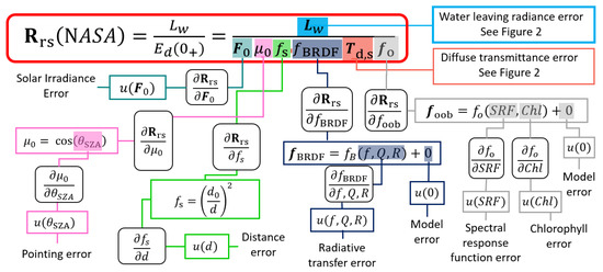
Figure 1.
In-band remote sensing reflectance () uncertainty tree diagram. Here, branches are given for solar irradiance , angle normalisation (cosine of solar zenith angle), Earth-Sun distance normalisation , BRDF normalisation and out-of-band-effect normalisation .
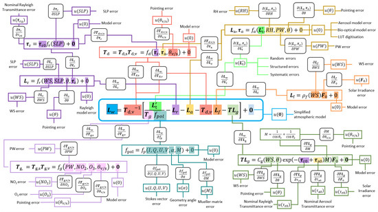
Figure 2.
Water-leaving radiance () uncertainty tree diagram. Here, branches are given for transmittances & , polarisation normalisation , and TOA (), Rayleigh (), aerosols (), foam () and glint () radiances.
There are many sources of measurement error identified in these uncertainty tree diagrams. In many cases, the full description of the analysis of an effect is beyond the scope of this work. Many of these uncertainty terms were studied in previous works (see [2] for a review). However, as far as we are aware, there were no previous studies into how much the atmospheric correction of ocean colour products is affected by uncertainties in ancillary parameters such as the surface wind speed (WS), sea level pressure (SLP), precipitable water vapour (PW), relative humidity (RH), nitrogen dioxide concentration ([]) and total ozone concentration ([]). The uncertainty tree diagrams allow an easy identification of the various modules of the algorithm where ancillary data have an impact. In Section 4, we will focus on these ancillary variable uncertainties and look at the spread in ancillary data in 2002. In the remainder of this Section, we briefly discuss for completeness the other uncertainty contributions for our two uncertainty tree diagrams. We refer to the ‘Uncertainties in Ocean Colour Remote Sensing’ review in [2] for a more detailed discussion.
3.2. Discussion of Uncertainty Contributions to Remote Sensing Reflectances
In this section, we discuss the contributions to the uncertainty tree diagram in Figure 1. When inspecting the measurement function, we see that a number of correction factors are applied to the water-leaving radiance to get the remote-sensing reflectance normalized for bi-directional effects (e.g., [22]), which is the fundamental measurement from which OC products, e.g., chlorophyll concentration, are derived. Each of these correction factors has an uncertainty associated with it.
The water-leaving radiances are normalised by the solar irradiance . The 1- uncertainty on is between 0.6 and 1.1%, depending on the wavelength [23]. This includes both random (0.5–1%) and systematic (about 0.25–0.5%) uncertainties. Another source of uncertainty is the pointing error on the solar zenith angle. These errors (including any interpolation errors, etc., for getting the solar zenith angle for a given pixel) are sufficiently small that the error on the correction factors can safely be considered negligible.
Additionally, there is a factor to correct the remote-sensing reflectance for variation in the Earth-Sun distance. The uncertainty on the earth-sun distance is well below 0.01% and can thus safely be considered negligible. The bidirectional reflectance distribution function (BRDF) effect is removed by correcting by a factor that depends on radiative transfer calculations. For a given set of geometry, wavelength, atmospheric conditions, and the chlorophyll concentration, the is taken from a look-up table. The magnitude of the error this introduces is generally unknown, and varies with existing conditions (e.g., [24,25]).
There is also an uncertainty associated with the out-of-band correction that is applied to the radiances in each band. This uncertainty comes from both an uncertainty in the spectral response function (SRF), and an uncertainty in the hyperspectral radiances (at the same spectral resolution as the SRF). The SRF is well defined with small uncertainties, but the hyperspectral radiances will vary from scene to scene. [26] derive a maximum of 0.8% model uncertainty on the correction factor at 555 nm for very clear open oceans. For the diffuse transmittance towards the sun and the water-leaving radiances , the uncertainty tree diagram refers to Figure 2, and these terms will thus be discussed in the next section.
3.3. Discussion of Uncertainty Contributions to Water-Leaving Radiances
Moving on to the measurement function for water-leaving radiances in Figure 2, we see the picture is a bit more complex, as many of the branches have their own measurement functions, which in turn have their own uncertainty contributions. For example, the first term (the diffuse transmittance from the surface to the instrument) has its own measurement function with associated uncertainty contributions, two of which in turn have their own branches on the uncertainty tree and their own measurement functions. To account for the uncertainty in our assumptions, we have again added ‘+0’ model error terms in the uncertainty tree diagram. The magnitude of these uncertainties is generally unknown.
The ancillary variables (WS, SLP, PW, RH, [O], and []) show up at the ends of multiple branches in the uncertainty tree diagram and thus errors in these parameters will have multiple effects (which might reinforce or counteract each-other) on the water leaving radiances. We discuss their uncertainties in Section 4. However, nitrogen dioxide is not included in Section 4 as it is not available from the ERA5 data, yet it does of course have uncertainties associated with it. Nitrogen dioxide has a fairly broad absorption spectrum with a peak at 412 nm. For this blue band, neglecting the [] would modify the TOA radiance by about 1% [27].
The gaseous transmittance is the product of the gaseous transmittance in direction of the sun and in the direction of the sensor and is determined by how much light the various gases absorb at each wavelength for these directions. only has uncertainty contributions from the ancillary variables and a pointing error that is negligible compared to the resolution of the reanalysis data. The pointing errors also show up in other branches and affect the values of , though these uncertainties are also small enough to be negligible. However, there is also a pointing uncertainty related to what the sensor is actually looking at. For a nonhomogeneous target, a small pointing error can still cause one to measure at a different location than expected.
The diffuse transmittance is the product of the diffuse transmittance towards the sun and in the viewing direction and it takes into account the light scattered out of the line of sight between the source and the sensor. The diffuse transmittance uncertainties are somewhat more complicated as depends on the Rayleigh and aerosol optical thickness, which have their own uncertainties. The Rayleigh optical depth and radiance are affected by errors in ancillary parameters, pointing errors, model errors and errors in the nominal Rayleigh transmittance. All but the latter have already been described in the previous paragraphs. One assumption made within SeaDAS is the wavelength-dependence of the nominal Rayleigh and aerosol transmittance functions. Any deviation from the assumed dependence will result in errors in the Rayleigh or aerosol radiances. Uncertainties on these were not estimated.
In addition to errors in the nominal aerosol transmittance, the aerosol radiances and optical depth depend on RH, PW, (negligible) pointing errors, model errors and errors in the TOA radiances (see next paragraph). There is also an additional source of uncertainty in determining the aerosol radiance/reflectance, which is due to the conversion from the multiple-scattering to the single-scattering , where is the ratio of aerosol reflectance at 2 near-infrared (NIR) bands [12]. The former is what can be constrained from the observations, yet the latter is the term used for the selection of the best aerosol model. The aerosol model selection is done using an iterative approach and look-up tables. This selection process has a significant uncertainty related to it, as the selected aerosol model may not faithfully represent the properties of the aerosols actually present (see also Section 6.2).
TOA radiances have both random uncertainties and systematic uncertainties which are typically on the order of 3–5% (e.g., [2,28]). Since the water-leaving radiances make up only a small fraction of the TOA signal, the uncertainties on the TOA radiances will be increased about tenfold when propagated to water-leaving radiances. Because of this, system vicarious calibration is typically used to reduce these uncertainties. A detailed discussion of the uncertainty budget of the TOA radiances is outside the scope of this document and was performed previously by e.g., [29] for SeaWiFS (see also [11,30] for a FIDUCEO-style approach for different TOA instruments). The random uncertainties come from detector noise, electrical noise, digitisation, cosmic rays, etc. The systematic uncertainties typically come from the calibration. Some of these biases apply to the whole image. Examples of this are errors from instrument characterisation, e.g., non-linearity characterisation, which are applied throughout the mission. There are also systematic uncertainties that apply on intermediate scales resulting in structured errors with nontrivial covariance structures. Stray light for example can make it into the detector and affect certain pixels more than others (depending on the instrument geometry).
The branch for the polarisation correction is relatively simple. This correction depends on the observed Stokes vector, the geometric angle, and the Mueller matrix (optical properties of the instrument). Each of these has uncertainties, which we cannot currently constrain. However, the total correction factor ranges from <0.25% for SeaWiFS to 3% for MODIS. Ref. [31] show that the polarization correction is acceptably accurate (to within 1%) when (key element in Mueller matrix) is independent of wavelength and less than about 0.1 in magnitude. For the remaining glint and foam radiance branches, all of the terms have already been discussed in previous paragraphs. However, model errors (+0 in the uncertainty tree diagrams) affecting these terms will be significantly different. Particularly, the assumed dependence of the foam and glint radiance on wind speed is particularly prone to model errors. Finally, even when the uncertainties on the input quantities are the same in different branches, the resulting uncertainties on the water leaving radiances will be different since the uncertainties propagate through different measurement functions.
4. Global Ancillary Variables
4.1. Statistics on Ancillary Variables
As illustrated in the uncertainty tree diagrams in Section 3, various ancillary data are necessary for the atmospheric correction from TOA radiances to remote-sensing reflectances. Before propagating the uncertainties on these ancillary data in following sections, it is important to understand the global variability of the ancillary data and their uncertainties. In this Section, we study the global ancillary data from NCEP and ERA5: their main characteristics are first presented and their differences are analysed; implications in terms of their uncertainties are then discussed. The goal of this section is to understand how representative the uncertainties we use in Section 6 are in a global context.
The five ancillary data considered here are WS, SLP, PW, RH and [O]. These variables are distributed in the NCEP data, except [O] provided by satellite missions such as TOMS. These variables are also directly available from the ERA5 data, except RH that can be computed from surface temperature () and dew point temperature () at 2 m altitude [32]:
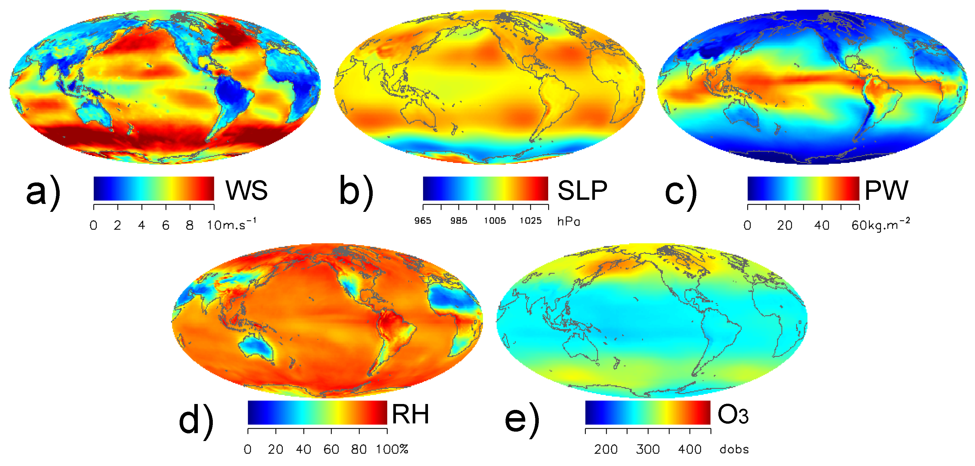
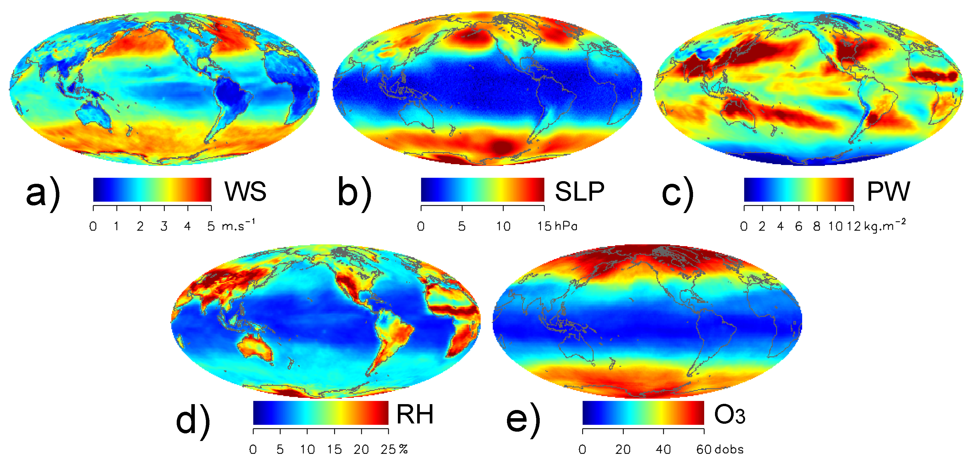
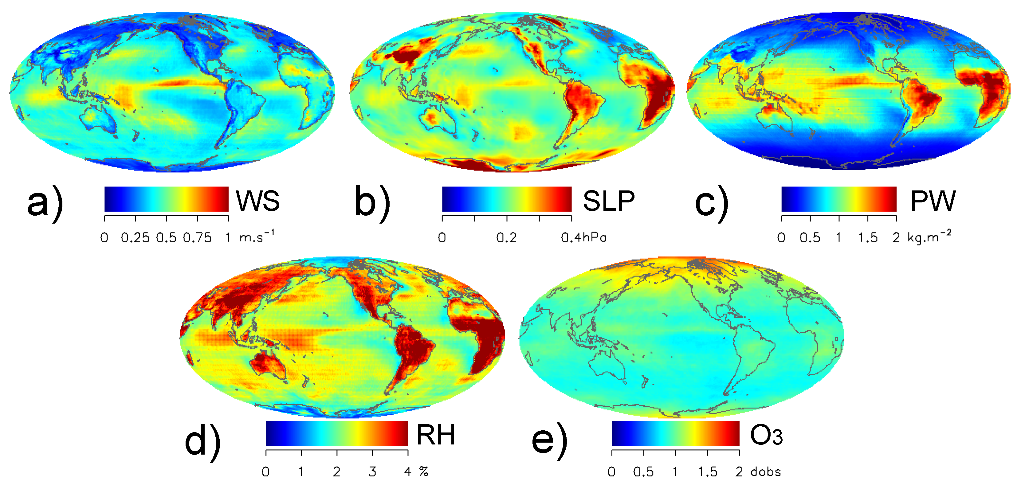
The annual average of the meteorological values (WS, SLP, PW and RH) from NCEP for the year 2002 are shown in Figure 3. They display well-known patterns of atmospheric circulation and dynamics (e.g., trade winds, high wind speeds in the Southern Ocean, high pressure systems in the subtropical gyres, high PW in the Inter-Tropical Convergence Zone (ITCZ), low humidity over terrestrial deserts, etc), while [O] provided by TOMS shows the expected gradient of higher values toward the high latitudes (Figure 3e). The annual average of the meteorological values is very similar for ERA5 (not shown). To document the natural variability of these quantities, their annual standard deviation is shown in Figure 4. Obvious features are the higher values found at mid-to-high latitudes for WS, SLP and RH whereas the standard deviation of PW shows distinct patterns at low and mid latitudes. For ozone, there is a strong gradient, with high values poleward of N.
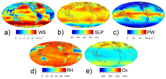
Figure 3.
Annual average for 2002 for NCEP meteorological variables: (a) surface wind speed WS, (b) sea level pressure SLP, (c) precipitable water vapor PW, (d) relative humidity RH, and (e) ozone concentration [O] from TOMS.

Figure 4.
Standard deviation for 2002 for NCEP meteorological variables: (a) surface wind speed WS, (b) sea level pressure SLP, (c) precipitable water vapor PW, (d) relative humidity RH and (e) ozone concentration [O] from TOMS.
Before further analysing the data from NCEP/TOMS and ERA5, statistical metrics are introduced. First, for a given grid point and time step j, the average of the ERA5 ensemble members () is expressed as:
where is the number of ensemble members (10 in the case of ERA5). The corresponding standard deviation of the ERA5 ensemble members (quantifying the ensemble spread) is written as:
The root-mean-square (RMS) deviation of is computed over the time steps of the year:
giving an average estimate of the spread between the ensemble members. As discussed in Section 2.3, the spread between ERA5 ensemble members gives a useful estimate of the uncertainties, though likely underestimating systematic uncertainties.
As mentioned above, the global average values from ERA5 are similar but not identical to those of NCEP/TOMS. The annual average of the differences between data from the two data sources is computed as (using the ensemble average in the calculation):
The difference between ERA5 and NCEP/TOMS is of course not constant and varies from day to day. To quantify this variability, the metric is introduced, quantifying the RMS difference between the 2 products (again using the ensemble average in the calculation):
Focusing first on the average ensemble spread, an important result is that shows distinct patterns for all five variables considered (Figure 5). A recurring feature is that high values of over the oceans are found near the equator (extending to higher and lower latitudes for the west Pacific and east Indian Ocean), except for [O] (Figure 5e). The values of exceed 0.75 m s for WS and 1.5 kg m for PW. Patterns of secondary magnitudes are seen in the northwest Pacific for WS, SLP and RH and the southern Pacific (about half way between New Zealand and Chile) for WS and SLP. For [O], high are distributed at high latitudes. In Section 6, we will look at how the spread between the ensemble members propagates to remote sensing reflectances. It is important to keep in mind that the results in Section 6 are only a local snapshot of the global variability reported in Figure 5.
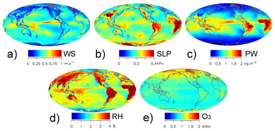
Figure 5.
Average ensemble spread for 2002 for (a) surface wind speed WS, (b) sea level pressure SLP, (c) precipitable water vapor PW, (d) relative humidity RH, and (e) ozone concentration [O].
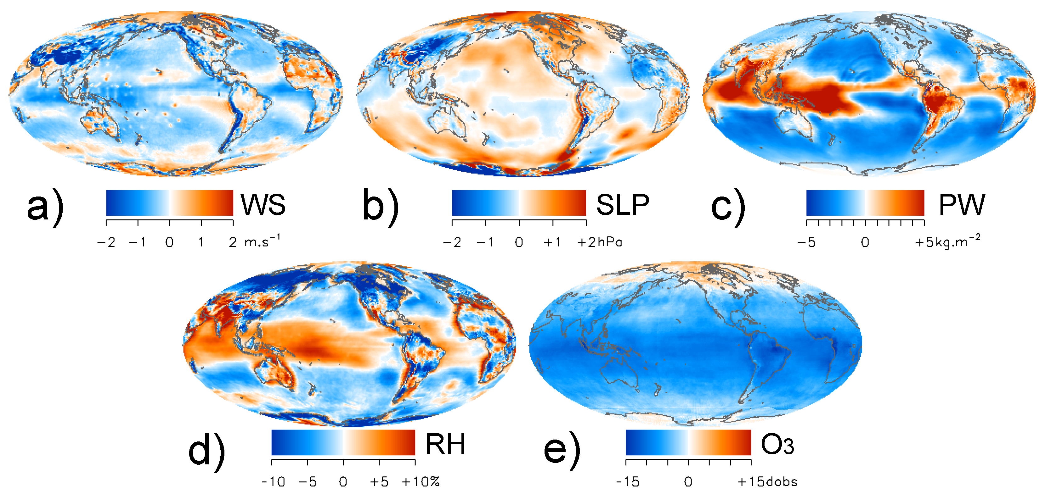
Figure 6 illustrates the RMS difference between the products of the two considered data sources, while Figure 7 shows the average difference . With respect to the ensemble spread , usually has higher amplitudes (comparing the colour scales of Figure 5 and Figure 6; see also median values reported in Figure 8). Even the amplitude of (in modulus) in Figure 7 is at least comparable or higher (particularly for [O]) than . The spread within the ERA5 ensemble is thus smaller than the differences between ERA5 and NCEP/TOMS. This is either because there are biases affecting the ERA5 and/or NCEP/TOMS data, or because ERA5 uncertainties are underestimated, with the ensemble not fully accounting for contributions of systematic terms to uncertainties.
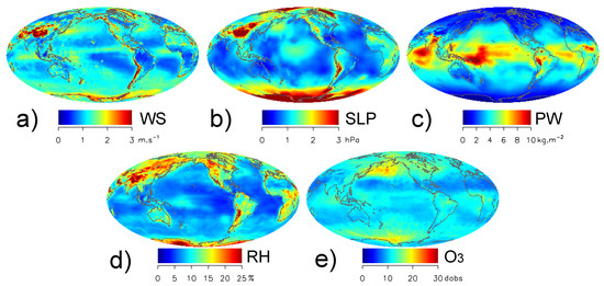
Figure 6.
RMS difference between ERA5 and NCEP/TOMS for 2002 for (a) surface wind speed WS, (b) sea level pressure SLP, (c) precipitable water vapor PW, (d) relative humidity RH, and (e) ozone concentration [O].
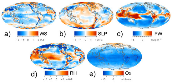
Figure 7.
Average difference between ERA5 and NCEP/TOMS for 2002 for (a) surface wind speed WS, (b) sea level pressure SLP, (c) precipitable water vapor PW, (d) relative humidity RH, and (e) ozone concentration [O].
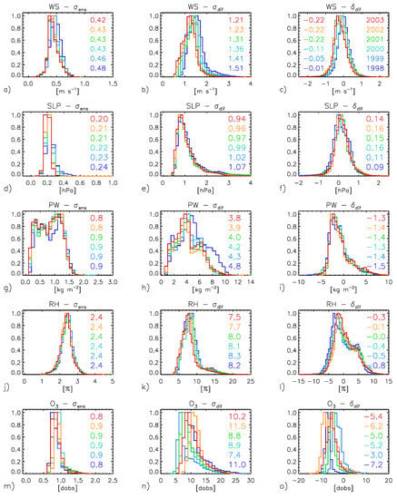
Figure 8.
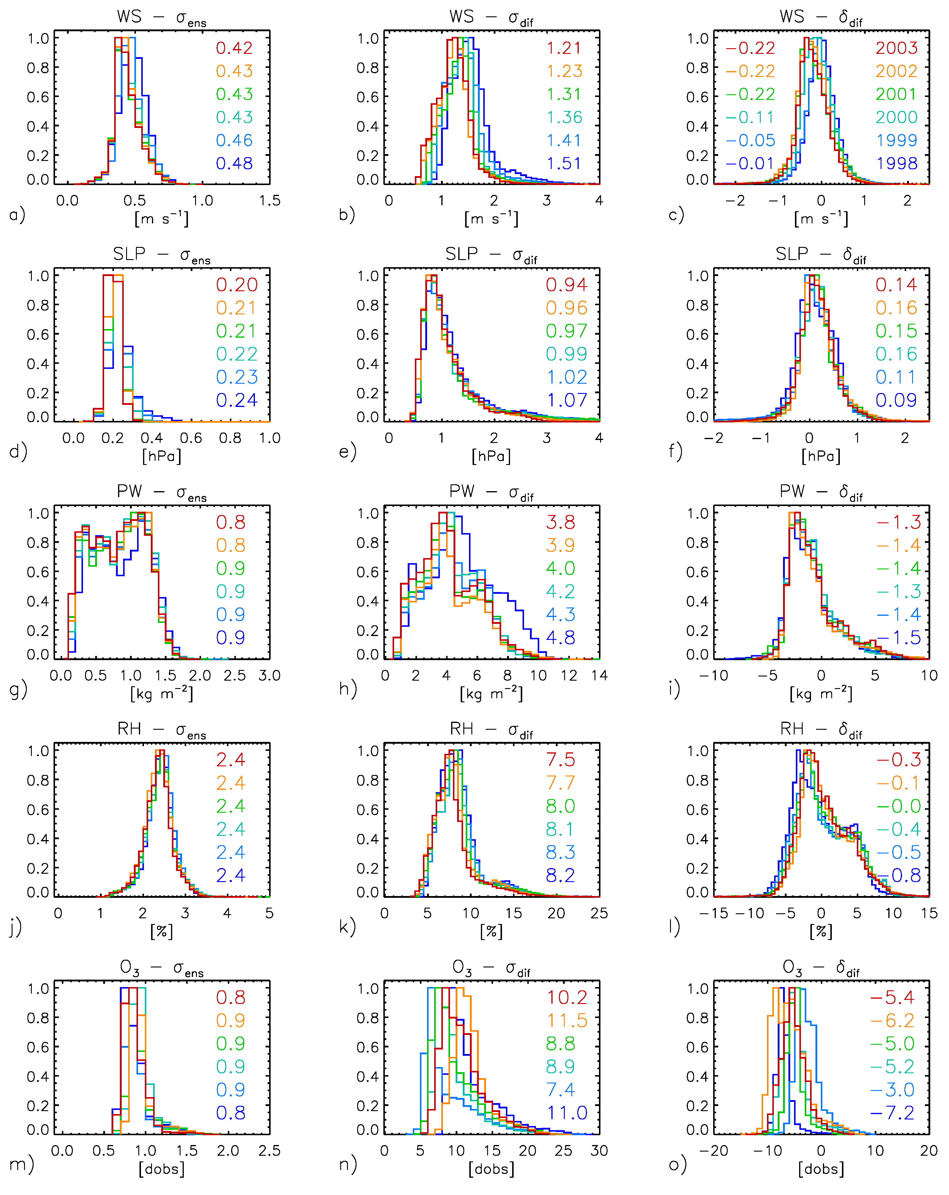
Frequency distributions of statistics (a,d,g,j,m) , (b,e,h,k,n) , and (c,f,i,l,o) for years listed in panel (c) and variables: (a–c) surface wind speed WS, (d–f) sea level pressure SLP, (g–i) precipitable water vapor PW, (j–l) relative humidity RH, and (m–o) ozone concentration [O]. Numbers provide median of every distribution for each year listed in panel (c).
Another important point is that the spatial distributions of and share some common patterns. For WS, in both cases, higher values are found for example in the equatorial Pacific and equatorial (east) Indian Ocean and the northwest Pacific, while low values are seen in the subtropical southern Pacific and Atlantic (Figure 5a and Figure 6a). One notable difference is that in the south of the Southern Ocean, the differences between NCEP and ERA5 are significantly more pronounced than for . For both data sources, higher values are observed in the Southern Ocean and the north Pacific for SLP, in the subtropical regions for PW, and in the tropical Indian and western Pacific regions for RH. In the case of [O], the highest are observed at high latitudes for both data sources. Some of the differences observed for [] are due to differences in how the data products were produced. ERA5 is a real daily average, whereas the TOMS product is a daily composite where each region is observed once at different times of the day.
Looking at in Figure 7, WS from ERA5 is on average lower than NCEP with some noticeable exceptions such as the Southern Ocean, eastern subtropical Pacific or the Arabian Sea. For SLP, is mostly positive, with local exceptions in the Pacific and western Indian Ocean. The values of for PW are mostly negative (ERA5 below NCEP) outside the tropics and south of the equator in the eastern Pacific and Atlantic, while it is positive in the rest of the tropics. Similarly for RH, is usually negative outside the tropics, and positive within the tropical band. As already anticipated by Figure 3, there is a latitudinal gradient in for [O], with the ERA5 product on average higher (lower) than TOMS in the high (low) latitudes. The overall agreement between the spatial distributions of and confirm our understanding that regions with high and are indeed regions of high uncertainty.
An important question is to know how these statistics and geographical patterns observed for 2002 change with time. From similar maps obtained for the period 1998–2003, the main patterns are actually well preserved every year (not shown). Figure 8 illustrates this agreement by showing frequency distributions and (ocean) median values that are very stable in time. To give further perspective to these results, it is worth comparing the median and with the standard deviation of the individual quantities over the year (that quantifies the natural variability). For WS and PW, the ratios between and the annual standard deviation are ∼0.1–0.15 while they are 0.47 for . These ratios are smaller for SLP, 0.04 and 0.19 for the ratios for and respectively, while they are higher for RH: the ratio between and the annual standard deviation is 0.3 while the median and annual standard deviation are almost equal, ∼8%. For [O], the ratio between and the annual standard deviation is 0.04 while the ratio of and annual standard deviation is about 0.5. So, even though usually smaller, the ERA5 ensemble spread or the difference between data sets are certainly not negligible with respect to natural variability, and they are in some cases comparable.
4.2. Ancillary Variables Uncertainties
In this section, we briefly review how the ancillary variables affect the atmospheric correction, and provide information on uncertainties documented for these quantities, and how they relate to the statistics presented in the previous section. A comprehensive discussion is also given by [2].
Surface wind speed (WS) is a key variable for performing an accurate atmosphere correction. It affects the shape (waves) and roughness of the sea surface, which directly affects the Rayleigh radiance (), the glint radiance () and whitecaps and foam radiance (), and indirectly the aerosol radiance (see also Section 6.2). Breaking waves can also introduce bubbles below the surface and thus modify the in-water radiation field. Comparing Numerical Weather Prediction monthly model products and buoy data from the tropical regions, Ref. [33] document RMS differences of the order of ∼1 m s but higher values would be expected for 6-h products. Ref. [34] show maps of RMS difference of model outputs and scatterometry satellite data, with values typically of 2 to 4 m s, higher values being seen in the high latitudes and ITCZ, patterns that are also observed for and (Figure 5a and Figure 6a) (see also [35]). Misfits with respect to observations of the order of 2 m s for only the zonal component of the wind are represented by [7] for ERA5 products. These values are fairly consistent with the distribution obtained for with a median 1.2–1.5 m s (Figure 8b), while might appear somewhat low with respect to actual uncertainties (with a median three times lower than that of ).
Sea level pressure is also an important variable for performing the atmosphere correction for ocean colour data. It affects the amount of gas molecules in the lines of illumination and sight, with a direct impact on Rayleigh scattering [36] and the atmospheric transmittance. Statistics shown above for or show larger values for the Southern Ocean, in line with the results of [37] who compared products from meteorological models. From comparison with island data, these authors obtained RMS differences of the order of 0.5–2 hPa with the largest values at high latitudes. For ERA5 products, [7] obtain misfits with respect to observations of the order of 0.6 hPa. So, with median values of 0.21 and 0.96 hPa, respectively (Figure 8d,e), and are consistent with these uncertainty estimates (with the former again at the low end).
Water vapour absorbs significant amounts of radiation within its absorption bands in the visible and near-infrared spectral range. This affects the gaseous transmittance and thus the process of atmospheric correction. For most OC instruments, the spectral bands were chosen to minimise overlap with the water absorption bands, yet there is still a non-negligible effect of water absorption, especially for nm. Besides transmittance, PW also affects the calculations of the aerosol radiance through out-of-band corrections active in the conversions between single and multiple scattering performed in SeaDAS. Using a diverse source of field data, results have shown RMS differences with meteorological products of the order of 1–2 kg m in the polar regions, 1.5–4 kg m in temperate regions and 2.5–6 kg m in the tropics [38,39,40], a latitudinal distribution that is consistent with that seen for or , and magnitudes comparable to and (ocean global median of 0.8 kg m and 3.9 kg m respectively, Figure 8g,h).
Within the SeaDAS processing chain, relative humidity (RH) is an important parameter as it is used in defining the aerosol models used in the atmospheric correction. The algorithm offers 80 candidate aerosol models, organized with 10 values of the aerosol fine-mode fraction and 8 values of RH [41]. First, the two families of aerosol models with RH bracketing the input value are kept for further analysis, the final selection being on the basis of the aerosol reflectance ratio of two bands in the near-infrared (NIR). Since the aerosol radiance () can make up a significant fraction of the TOA radiance (), RH has the potential to significantly affect the calculated water leaving radiance. Misfits with respect to observations of the order of 10% were seen for ERA5 products [7], and other studies comparing products (including satellite-based ones) suggest that this is not uncommon [42,43]; even the uncertainty of some in-situ measurements may reach this value [44]. Values of 10% are also fairly typical for over the oceans (having an ocean global median of 7.7%) while is usually lower (median of 2.4%) (Figure 8j,k).
Ozone absorbs light between 500 and 700 nm with a peak at 600 nm and thus affects the gaseous transmittance. Ozone satellite products typically have uncertainties below 5% [16,45,46] that correspond fairly well to the differences between ERA5 and TOMS as quantified by (ocean global median of 11.5 dobs, Figure 8n). The ERA5 ensemble spread is smaller (ocean global median of 0.9 dobs, Figure 8m).
As already noted, is usually lower than . Some elements suggest that at least some ensemble spreads within the ERA5 ensemble are too small with respect to actual uncertainties [47], and the low values of with respect to are at least partly explained by the fact that does not include any systematic terms that would contribute to a general uncertainty budget. In the case of ERA5, higher values of and, in general, of the products uncertainties are expected when the availability of in-situ data is low for assimilation in the re-analysis simulations, which might contribute for example to the high values found for SLP in the Southern Ocean. However, due to including a wide range of satellite records, for such regions ERA5 has significantly smaller uncertainties than its predecessors such as CERA-20C ([47]; see also Mélin et al., submit.). Considering , it is obvious that both products (ERA5 or NCEP/TOMS) cannot be true at the same time, but implications for the uncertainties of the individual products are not straightforward. The fact that both distributions ( and ) are stable in time and share major spatial patterns, and that they are comparable to uncertainty values reported in published studies suggest that they can be considered as representative estimates of uncertainties for the considered ancillary variables, with usually on the low end. It practically means that they can be used to test the sensitivity of the atmospheric correction to uncertainties in ancillary variables.
5. Uncertainty Propagation Method
As discussed in Section 4.1, there is a lot of spatial variability in the uncertainties on each of the relevant ancillary parameters. There are also temporal changes. Therefore, to get realistic uncertainty estimates on the remote sensing reflectances, it is important to get a local estimate of the ancillary data uncertainties at the relevant time (time of satellite overpass), consistent with the combination of observations available at that time and location. Reanalysis datasets are the best option to obtain such data, as they assimilate all available observations by design and combine them into a consistent framework (and with representative uncertainty information in the case of ERA5, see previous section). We thus opt to use the ERA5 ensemble to obtain uncertainty estimates on the input quantities (i.e., the ancillary data) in our uncertainty propagation. The 10-member ensemble is a new inclusion in this recently updated ERA dataset. It provides the most detailed information in terms of uncertainty for any reanalysis dataset.
To perform the correction from TOA radiances to surface reflectances, it is possible to give SeaDAS input files containing ancillary data specified by the user. These files need to be in HDF format mimicking the NCEP data. To use the ERA5 ensemble members, we thus first need to convert the ERA5 ancillary data to NCEP format. We produce two files (one for ozone and one for the other ancillary variables, as required by SeaDAS) for each ensemble member and each time frame (every three hours). ERA5 has a finer resolution than the NCEP data. Therefore, we resample the ERA5 data to the same grid as the NCEP data.
A Monte Carlo (MC) approach is used to propagate the uncertainties in the ancillary data to the remote sensing reflectances. MC methods typically generate a large number of draws from an input probability distribution and propagate each draw through the measurement function. The resulting output values then make up an approximation of the output probability distribution, which in turn can be used to determine uncorrelated and correlated uncertainties in the measurand. For our study, we use the whole SeaDAS level 1 to level 2 processing chain as the measurement function.
Usually many draws are generated from the input distribution. However, ERA5 only has 10 ensemble members (due to the large computational cost per ensemble member), which together make up the best available probability distribution. We thus use the 10 members as 10 individual MC draws. For each level 1 scene, we generate 10 level 2 maps corresponding to the 10 ensemble members. We then study the standard deviation in each pixel between these 10 level 2 maps and compare it to the standard deviation within the corresponding ancillary data in the ensemble.
The various ancillary data variables each influence the measurement function shown in Figure 2. The level 2 uncertainties will thus have some contribution from each of the included ancillary data variables. It is very difficult to disentangle these contributions without additional information. Therefore, we performed a second set of MC analyses, where only one of the ancillary data variables is varied at once. The other parameters are not varied and kept to the ensemble average. By varying the ancillary data one variable at a time, we can separate the contributions of the various ancillary data to the level 2 uncertainty in each pixel. We then look at the correlation between the pixel uncertainty in the level 2 maps and the pixel ancillary data uncertainty on the same scale. For the latter, we use the interpolated ancillary data maps produced by SeaDAS which are on the same grid as the level 1 and level 2 maps.
6. Remote Sensing Reflectance Uncertainties
6.1. Relative Uncertainty at Different Wavebands
To study the uncertainty introduced by the ancillary data, we make maps of the standard deviation (std) between the propagated ensemble members for each waveband. In Figure 9, we show images of the average 555 nm remote-sensing reflectance (), as well as the relative std in each pixel (i.e., standard deviation between ensemble members, divided by ensemble average). We see that in some regions, the relative std is around 2%, yet in most of the image it is significantly lower. In addition to studying the std between the ERA5 ensemble members, we can also look at the differences between the ensemble average and the NCEP-based data in Figure 9 (right). The differences are somewhat larger than between the ERA5 ensemble spread.
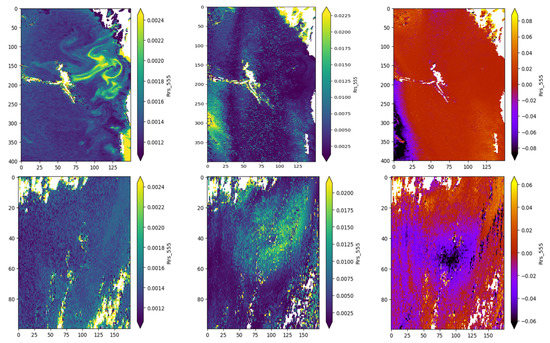
Figure 9.
Average 555 nm remote-sensing reflectance (left), relative standard deviation (centre) between ensemble members, and relative difference between NCEP and ERA5 (right) for Australian scene consisting of MLAC (1.1 km) pixels (top), and Atlantic scene consisting of GAC (4 km) pixels (bottom).
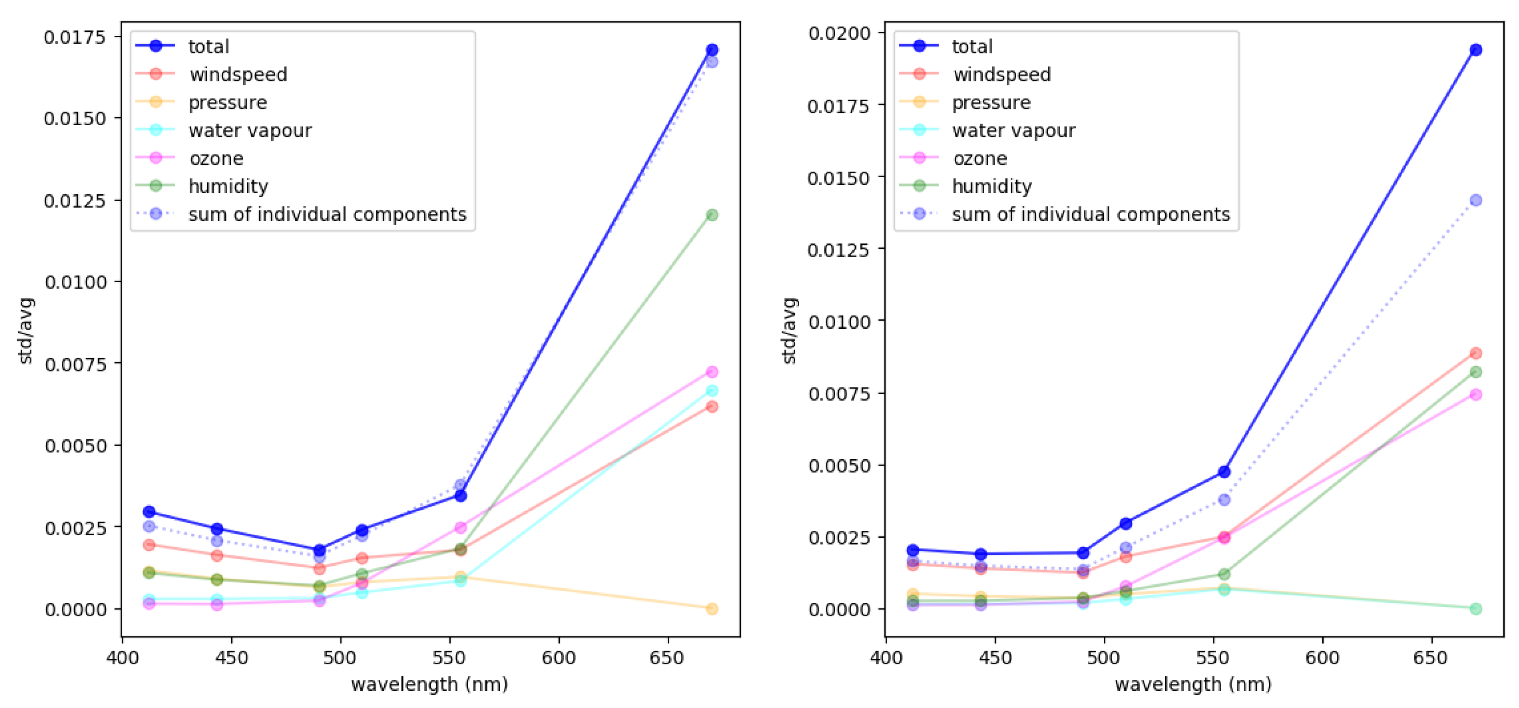
We can quantify the differences between images by looking at the median pixel of the relative std images (i.e., the median of the relative std between ensemble members for each pixel). For the relative std between ERA5 ensemble members (Figure 9 centre), the median pixel corresponds to 0.5% for the Australian scene, and 0.6% for the Atlantic scene. The medians of different wavebands can be used to study the wavelength dependency of the remote sensing reflectance uncertainties. Figure 10 shows the total relative std from varying all ancillary parameters at once as the blue line. The 670 nm waveband has significantly higher std than the blue bands, and the 555 nm waveband has slightly higher values too. In relative terms, the red bands are thus more susceptible to uncertainties introduced by the ancillary data.
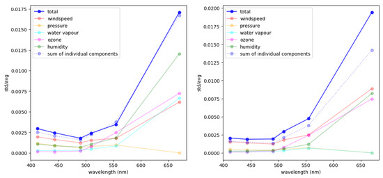
Figure 10.
Plots showing wavelength-dependence of median pixel for Australian scene (left) and Atlantic scene (right). Various coloured lines show relative std for varying all ancillary variables at once, relative std for varying variables one-by-one, and quadratic sum of individual components.
Figure 10 also shows the relative std from varying the ancillary variables one-by-one, and the quadratic sum of the individual components for the median pixel in each band. When we compare the individual contributions, we see that for the blue bands WS is the dominant contribution for both scenes. For the red bands, RH is the biggest contributor for the Australian scene, yet WS is still the biggest contribution for the Atlantic scene (closely followed by RH). [] is also an important contributor for the red bands. SLP does not add much variance in any of the bands. The effect of PW is quite different for our two scenes. For the Australian scene, PW is a significant contributor in the red bands, yet for the Atlantic scene it only adds a very small contribution. We also note in Figure 10 that the total relative std is similar to the quadratic sum of the individual components. This indicates that the different contributions are fairly uncorrelated to each-other.
To understand how to put these results in a global context, we can compare where our ancillary data lies within the global distribution discussed in Section 4.1. In Table 1, we list the range of the ancillary data within our two scenes as well as the range of their uncertainties. When these are compared with their respective regions in Figure 3, we find that compared to the annual average, both scenes have lower WS, slightly lower RH, slightly lower PW and similar []. The SLP for the Australian scene is lower than the annual average, yet for the Atlantic scene it is similar. The differences with the annual average could be due to a bias introduced by our selection criteria of the scene having a large clear-sky area or simply due to the specific meteorological regimes analysed at the time (which would be expected to differ from the annual average values for most times). In addition, we can also compare the uncertainties to the global distribution of . The spread between the ensemble members for the pixels in our scenes lie well within the global distributions for 2003 in Figure 8, with the exception of the PW uncertainty for the Atlantic scene, which has significantly higher values. The reason for this high spread between ensemble members for PW for this scene is not clear. Compared to the annual average value of their respective locations in Figure 5, a similar picture emerges, where now the values in Table 1 for the Atlantic scene are somewhat lower for WS and again higher for PW, but all the other values are comparable. We will revisit the ancillary variables within a global context in a dedicated study (Mélin et al., submit.), where we perform a much more systematic study on global scales.

Table 1.
Table listing range of pixel values of ancillary parameter values for each of our two scenes.
6.2. Sensitivity to Aerosol Model Selection
If we look at the std in Figure 9 (centre column) in more detail, we see that the introduced variation is not smooth, and there are some pixels that seem to have significantly higher std than the surrounding pixels, whereas we know that the variation in each of the ancillary parameters varies smoothly. In this section, we look at what affects these pixels, as it will influence the discussion in the following sections. We here focus our discussion on the Australian scene, although the same principles apply to other scenes too.
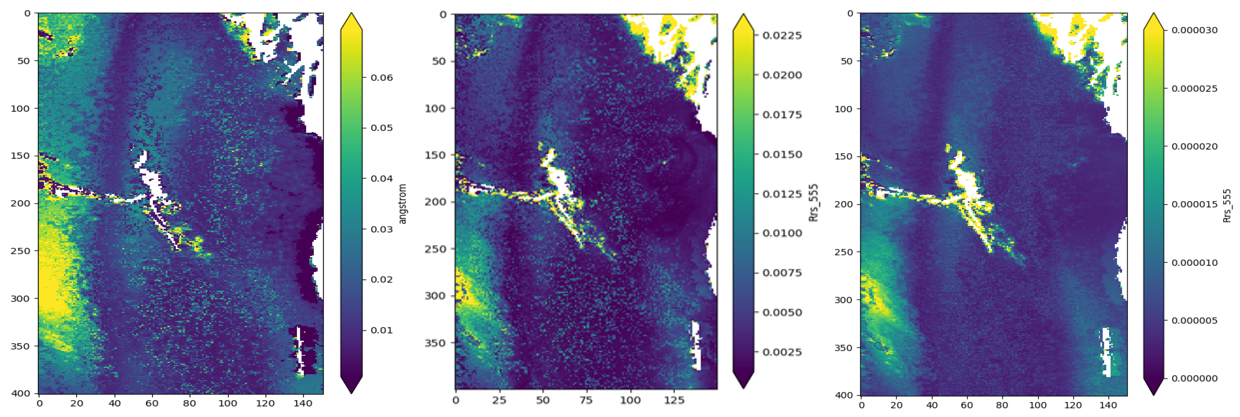
The reason for the large std in these pixels becomes clear when we look at the std in the Ångström exponent , the slope of the aerosol models. By manually inspecting the outlying pixels in the left and centre panels of Figure 11, it can be seen that the outlying pixels are the same in the Ångström std as in the remote-sensing reflectance std. It is thus a difference in aerosol model selection (between the different ensemble members for that pixel) that causes these outlying pixels. To better understand this, we look in more detail at how the aerosol models are selected. The main factors in selecting an aerosol model are the RH, and the observed (again, the ratio between NIR aerosol reflectance). The RH mainly serves in limiting which aerosol models are compared to the observed . When the observed RH goes across a tabulated RH value associated with a subset of the candidate aerosol models, significant changes in the calculation of the aerosol radiance might happen but this effect does not explain the large pixel-to-pixel variations in std as the RH variability is very smooth (being interpolated from 1-degree resolution products).

Figure 11.
Relative std between ensemble members for aerosol Ångström exponent (left), 555 nm remote sensing reflectance without adding noise (centre), and 555 nm reflectance after adding measurement noise to each L1 map and averaging, resulting in std maps between members (right).
The observed corresponds to the total Multiple Scattering (MS) , whereas the aerosol models are characterised by Single Scattering (SS) . Even though the polynomial functions to convert the model SS to model MS were computed for each model, the comparison of the MS observed to the SS model is complicated by two effects. The first is that the diffuse transmittance, which is applied when calculating the observed MS , is dependent on which aerosol model is selected. Second, the conversion from model SS to MS is not only model-dependant but also depends on the observed radiances (after correcting for glint, foam and Rayleigh radiances). Several methods were developed to deal with this. We use the default SeaDAS option, which is the RH-dependent [12] aerosol model selection, for which the model selection is done iteratively. Starting with all models at a given RH, the algorithm determines an average observed SS by converting the observed MS to a SS for each model, and then removes the two models that are furthest away from the average SS . A new average SS is then calculated, and the process is repeated until only 2 models remain. An interpolation is then performed between these 2 models.
The key cause of the observed variance here is that around some critical values between two models, slight variations in the observed MS (due to changes in, e.g., the transmittance), can lead to a different average and different models being discarded, which then affects the next average. A small change can thus cause a large difference, but only if the observed MS (which is affected by the noise in the L1 maps) is close to some critical transition value that causes different models to be discarded during the selection. This explains how only few pixels are affected by this issue.
One way to mitigate the variance introduced by this is by adding noise to the L1 observations and averaging the results. For each L1 map, we generate 10 new maps following a Monte Carlo approach and a 0.1% L1 uncertainty. After processing each of the generated L1 maps with SeaDAS for each member in the ERA5 ensemble, we calculate the std between the different members for the same L1 map. Next, we average the std maps for each generated L1 map. This spreads out which pixels are at the critical transition value and leads to smoother std maps, as illustrated in the right panel of Figure 11. Adding noise will allow to produce smoother maps which make it easier to visually reveal the underlying correlations with ancillary data and will give us a better measure for the average uncertainty in a pixel. Following the standard approach without adding measurement noise will result in some pixels being quite strongly biased (up to about 1%), while other pixels are unaffected. The latter can be useful for better revealing trends in the unaffected pixels. Both versions of the maps can thus be useful, yet throughout the remainder of this document we use the version without adding additional noise.
6.3. Spatial Correlation between Variance in Ancillary Data and Reflectance
Next, we look at the spatial correlation between the uncertainty in the ancillary data and the associated uncertainty in the remote sensing reflectances. We show in Figure 12 the spatial correlation between the standard deviation (between the 10 ERA5 ensemble members) in WS and the standard deviation in the resulting L2 maps when only WS is varied for both scenes. We find a strong linear correlation for all except the red band (correlation coefficient ranging from for 412 nm to for 555 nm when strong outliers are discarded) between the uncertainties in WS and the associated uncertainties in the remote sensing reflectances. However, from analysing additional scenes, we find that this clear correlation does not hold for all scenes (especially for high WS).
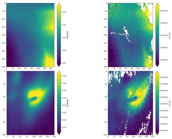
Figure 12.
Plots illustrating uncertainty on WS (left) and associated uncertainty on remote sensing reflectance (right) for our Australian Scene (top) and Atlantic Scene (bottom).
RH, which is the other main contributor to the uncertainty on remote sensing reflectances, does not have such a clear spatial correlation (at least on the pixel-level) since the RH affects the aerosol model selection through rather complex selection criteria which also depend on other parameters.
There is a strong linear correlation between the std in SLP and the std in 412 nm reflectance (correlation coefficient ranging from at 412 nm to at 555 nm). However, this strong linear correlation between most pixels in Figure 13 is not easily visible due to the strong outliers. There are again two uncertainty components when varying SLP only: one accounting for the uncertainty arising from std in the Rayleigh radiance and transmittances, and one accounting for the outlying pixels due to the aerosol selection. The critical transition for aerosol model selection uncertainty is very apparent here due to the lower overall variance in the image from the other component (as the uncertainty on SLP itself is very low). The pixels that are at the critical transition values stand out much more.
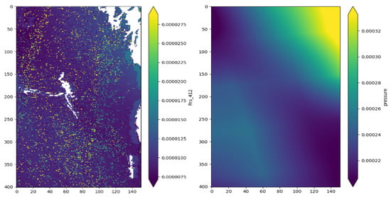
Figure 13.
Plots illustrating dependence of remote sensing reflectance on SLP for Australian Scene.
PW and [] also contribute to the uncertainty budget, yet do not show clear spatial correlations between the std in the ancillary parameters and the std in the resulting reflectance maps. For both these variables we also find a continuous component as well as outliers due to some pixels being around critical transition values for aerosol model selection.
The results presented in this section are based on representative SeaWiFS images but it is acknowledged that they are susceptible to vary for other areas and/or periods and that a much larger study is required (see Mélin et al., submit.).
7. Conclusions
We illustrated the uncertainty budget of the NASA SeaDAS l2gen software using an uncertainty tree diagram and discussed the various uncertainty contributions. From the uncertainty tree diagram, the components of the algorithm where ancillary data have an impact were identified. To judge the effect of the ancillary data uncertainties in the atmospheric correction, an MC approach was used where the MC steps were taken to be the 10 members of the ERA5 ensemble. Our main conclusions from this study are:
- The SeaDAS uncertainty budget reveals numerous sources of error. Particularly, ancillary data uncertainties enter the measurement equation through various branches and together form an important contribution to the uncertainty budget.
- The difference between the NCEP/TOMS and ERA5 ancillary data is larger than the variance within the ERA5 ensemble. Both the average difference between NCEP/TOMS and ERA5 and the spread within ERA5 show similar spatial patterns, with the largest values generally observed in the the mid-latitudes for surface wind speed (WS), sea level pressure (SLP), precipitable water vapour (PW), and relative humidity (RH) or the high latitudes for total ozone concentration ([]). Differences between ancillary data and within the ensemble appear to provide realistic estimates of their uncertainties in magnitude and spatial distribution, and allow sensitivity analyses on OC data processing. However, these uncertainty estimates might be slightly underestimated due to the ensemble spread not fully including systematic effects.
- WS and RH (through its interaction with aerosol model selection) were found to be the biggest contributors to the uncertainty in the atmospheric correction.
- The complex iterative aerosol model selection algorithm leads to a small fraction of pixels having significantly higher uncertainties than other pixels. This happens when the L1 radiances (of the bands used in aerosol model selection) for these pixels are near some critical transition values, which results in a different model being selected for different MC iterations.
- The uncertainties in the remote sensing reflectance due to WS and SLP typically show a strong spatial correlation with the uncertainties in WS and SLP, respectively. The other ancillary variables show no such strong correlation.
- The uncertainty in remote sensing reflectances introduced by varying RH is complex. In addition to the pixels close to the critical transition values, aerosol model selection also introduced large-scale variation in uncertainties.
In general, it is thus recommended that uncertainties on ancillary variables (especially those on WS and RH) are included when determining uncertainties on ocean colour remote sensing reflectances. For a more detailed global picture, we refer to Mélin et al., (submit.). In future work, it would be very interesting to study the effects of ancillary data uncertainties on water quality parameter estimations (such as chlorophyll-a) as well as to explore other algorithms for retrieving remote sensing reflectances, especially if the effects of aerosols and their detailed dependence on RH can be better understood.
Author Contributions
Writing—original draft preparation, P.D.V.; writing—review and editing, F.M., S.E.H., R.M., M.S. and B.B.; conceptualization, P.D.V., F.M. and S.E.H.; methodology, P.D.V., F.M. and S.E.H.; formal analysis, P.D.V.; investigation, P.D.V., F.M., S.E.H., R.M., M.S.; visualization P.D.V. and F.M. All authors have read and agreed to the published version of the manuscript.
Funding
The authors gratefully acknowledge funding from the MetEOC-3 and MetEOC-4 projects (in turn funded under EMPIR grant 16ENV03 and 19ENV07 respectively). The EMPIR initiative is funded by the European Union Horizon 2020 research and innovation program and cofinanced by the EMPIR participating states.
Data Availability Statement
The L1 SEAWIFS data and NCEP reanalysis data used in this study are provided by the NASA Goddard Space Flight Center, Ocean Ecology Laboratory, Ocean Biology Processing Group. The SEAWIFS level 1 data (https://oceancolor.gsfc.nasa.gov/data/10.5067/ORBVIEW-2/SEAWIFS/L1/DATA/1/) was downloaded using the https://oceancolor.gsfc.nasa.gov/cgi/browse.pl?sen=swga and the NCEP data was manually downloaded from https://oceandata.sci.gsfc.nasa.gov/Ancillary/Meteorological/. The ERA5 data were downloaded from the Copernicus Climate Change Service (C3S) https://cds.climate.copernicus.eu/ (CDS) [20].
Acknowledgments
The Ocean Biology Processing Group (OBPG) of NASA is acknowledged for the distribution of the SeaWiFS Level-1 data, as well as ancillary files for NCEP and TOMS/TOVS data. The Copernicus Climate Change Service (C3S), hosted by The European Centre for Medium-Range Weather Forecasts (ECMWF), is thanked for the availability of the ERA5 ensemble data that allowed this research. Finally, a special thanks to Agnieszka Bialek and Paul Green for useful discussion and comments.
Conflicts of Interest
The authors declare no conflict of interest.
References
- GCOS. The Global Observing System for Climate: Implementation Needs; GCOS-200; WMO: Geneva, Switzerland, 2016; p. 284. [Google Scholar]
- IOCCG. Uncertainties in Ocean Colour Remote Sensing; Reports of the International Ocean Colour Coordinating Group; IOCCG: Dartmouth, ON, Canada, 2019; Volume 18. [Google Scholar] [CrossRef]
- Gordon, H.R. Removal of atmospheric effects from satellite imagery of the oceans. Appl. Opt. 1978, 17, 1631–1636. [Google Scholar] [CrossRef] [PubMed]
- Ruddick, K.G.; Ovidio, F.; Rijkeboer, M. Atmospheric correction of SeaWiFS imagery for turbid coastal and inland waters. Appl. Opt. 2000, 39, 897–912. [Google Scholar] [CrossRef] [Green Version]
- Bailey, S.; Franz, B.; Werdell, P. Estimation of near-infrared water-leaving reflectance for satellite ocean colour data processing. Opt. Exp. 2010, 18, 7521–7527. [Google Scholar] [CrossRef] [PubMed]
- Kanamitsu, M.; Ebisuzaki, W.; Woollen, J.; Yang, S.K.; Hnilo, J.J.; Fiorino, M.; Potter, G.L. NCEP/DOE AMIP-II Reanalysis (R-2). Bull. Am. Meteorol. Soc. 2002, 83, 1631–1644. [Google Scholar] [CrossRef]
- Hersbach, H.; Bell, B.; Berrisford, P.; Hirahara, S.; Horányi, A.; Muñoz-Sabater, J.; Nicolas, J.; Peubey, C.; Radu, R.; Schepers, D.; et al. The ERA5 global reanalysis. Q. J. R. Meteorol. Soc. 2020, 146, 1999–2049. [Google Scholar] [CrossRef]
- Steinmetz, F.; Deschamps, P.Y.; Ramon, D. Atmospheric correction in presence of sun glint: Application to MERIS. Opt. Exp. 2011, 19, 571–587. [Google Scholar] [CrossRef] [Green Version]
- Shi, C.; Nakajima, T.; Hashimoto, M. Simultaneous retrieval of aerosol optical thickness and chlorophyll concentration from multiwavelength measurement over East China Sea. J. Geophys. Res. Atmos. 2016, 121, 14084–14101. [Google Scholar] [CrossRef]
- Frouin, R.; Pelletier, B. Bayesian methodology for inverting satellite ocean-colour data. Remote Sens. Environ. 2015, 159, 332–360. [Google Scholar] [CrossRef]
- Mittaz, J.; Merchant, C.J.; Woolliams, E.R. Applying principles of metrology to historical Earth observations from satellites. Metrologia 2019, 56, 032002. [Google Scholar] [CrossRef]
- Gordon, H.R.; Wang, M. Retrieval of water-leaving radiance and aerosol optical thickness over the oceans with SeaWiFS: A preliminary algorithm. Appl. Opt. 1994, 33, 443–452. [Google Scholar] [CrossRef]
- Franz, B.; Bailey, S.; Werdell, P.; McClain, C. Sensor-independent approach to the vicarious calibration of satellite ocean colour radiometry. Appl. Opt. 2007, 46, 5068–5082. [Google Scholar] [CrossRef] [PubMed]
- Pahlevan, N.; Sarkar, S.; Franz, B.; Balasubramanian, S.; He, J. Sentinel-2 MultiSpectral Instrument (MSI) data processing for aquatic science applications: Demonstrations and validations. Remote Sens. Environ. 2017, 201, 47–56. [Google Scholar] [CrossRef]
- Hooker, S.; Esaias, W.; Feldman, G.; Gregg, W.; McClain, C. An Overview of SeaWiFS and Ocean Colour; NASA Technical Memorandum 104566; NASA Goddard Space Flight Center: Greenbelt, MD, USA, 1992; pp. 1–24.
- McPeters, R.; Bhartia, P.; Krueger, A.; Herman, J.; Wellemeyer, C.; Seftor, C.; Jaross, G.; Torres, O.; Moy, L.; Labow, G.; et al. Earth Probe Total Ozone Mapping Spectrometer (TOMS) Data Products User’s Guide; NASA Technical Publication 1998-206895; NASA Goddard Space Flight Center: Greenbelt, MD, USA, 1998; p. 64.
- Bell, B.; Hersbach, H.; Simmons, A.; Berrisford, P.; Dahlgren, P.; Horányi, A.; Muñoz-Sabater, J.; Nicolas, J.; Radu, R.; Schepers, D.; et al. The ERA5 global reanalysis: Preliminary extension to 1950. Q. J. R. Meteorol. Soc. 2021, 147, 4186–4227. [Google Scholar] [CrossRef]
- Leutbecher, M.; Lock, S.J.; Ollinaho, P.; Lang, S.T.K.; Balsamo, G.; Bechtold, P.; Bonavita, M.; Christensen, H.M.; Diamantakis, M.; Dutra, E.; et al. Stochastic representations of model uncertainties at ECMWF: State of the art and future vision. Q. J. R. Meteorol. Soc. 2017, 143, 2315–2339. [Google Scholar] [CrossRef]
- Hirahara, S.; Alonso-Balmaseda, M.; de Boisseson, E.; Hersbach, H. Sea Surface Temperature and Sea Ice Concentration for ERA5; ECMWF: Reading, UK, 2016. [Google Scholar]
- Hersbach, H.; Bell, B.; Berrisford, P.; Biavati, G.; Horányi, A.; Muñoz Sabater, J.; Nicolas, J.; Peubey, C.; Radu, R.; Rozum, I.; et al. ERA5 hourly data on single levels from 1979 to present. In Copernicus Climate Change Service (C3S) Climate Data Store (CDS); ECMWF: Reading, UK, 2018. [Google Scholar] [CrossRef]
- Mobley, C.D.; Werdell, J.; Franz, B.; Ahmad, Z.; Bailey, S. Atmospheric Correction for Satellite Ocean Colour Radiometry; Technical Memorandum; NASA: Greenbelt, MD, USA, 2016.
- Morel, A.; Antoine, D.; Gentili, B. Bidirectional reflectance of oceanic waters: Accounting for Raman emission and varying particle scattering phase function. Appl. Opt. 2002, 41, 6289–6306. [Google Scholar] [CrossRef]
- Thuillier, G.; Hersé, M.; Labs, D.; Foujols, T.; Peetermans, W.; Gillotay, D.; Simon, P.C.; Mandel, H. The Solar Spectral Irradiance from 200 to 2400 nm as Measured by the SOLSPEC Spectrometer from the Atlas and Eureca Missions. Sol. Phys. 2003, 214, 1–22. [Google Scholar] [CrossRef]
- Voss, K.; Morel, A.; Antoine, D. Detailed validation of the bidirectional effect in various Case 1 waters for application to ocean colour imagery. Biogeosciences 2007, 4, 781–789. [Google Scholar] [CrossRef] [Green Version]
- Gleason, A.; Voss, K.; Gordon, H.; Twardowski, M.; Sullivan, J.; Trees, C.; Weideman, A.; Berthon, J.F.; Clark, D.; Lee, Z.P. Detailed validation of the bidirectional effect in various Case I and Case II waters. Opt. Exp. 2012, 20, 7630–7645. [Google Scholar] [CrossRef]
- Wang, M.; Franz, B.A.; Barnes, R.A.; McClain, C.R. Effects of spectral bandpass on SeaWiFS-retrieved near-surface optical properties of the ocean. Appl. Opt. 2001, 40, 343–348. [Google Scholar] [CrossRef] [PubMed]
- Ahmad, Z.; McClain, C.R.; Herman, J.R.; Franz, B.A.; Kwiatkowska, E.J.; Robinson, W.D.; Bucsela, E.J.; Tzortziou, M. Atmospheric correction for NO2 absorption in retrieving water-leaving reflectances from the SeaWiFS and MODIS measurements. Appl. Opt. 2007, 46, 6504–6512. [Google Scholar] [CrossRef] [PubMed] [Green Version]
- Barnes, B.; Eplee, R.; Schmidt, G.; Patt, F.; McClain, C. Calibration of SeaWiFS. I. Direct techniques. Appl. Opt. 2001, 40, 6682–6700. [Google Scholar] [CrossRef] [PubMed] [Green Version]
- Eplee, R.E.; Meister, G.; Patt, F.S.; Franz, B.A.; McClain, C.R. Uncertainty assessment of the SeaWiFS on-orbit calibration. In Earth Observing Systems XVI; Butler, J.J., Xiong, X., Gu, X., Eds.; International Society for Optics and Photonics; SPIE: Bellingham, WA, USA, 2011; Volume 8153, pp. 93–109. [Google Scholar] [CrossRef] [Green Version]
- Smith, D.; Hunt, S.E.; Etxaluze, M.; Peters, D.; Nightingale, T.; Mittaz, J.; Woolliams, E.R.; Polehampton, E. Traceability of the Sentinel-3 SLSTR Level-1 Infrared Radiometric Processing. Remote Sens. 2021, 13, 374. [Google Scholar] [CrossRef]
- Gordon, H.R. Atmospheric correction of ocean colour imagery in the Earth Observing System era. J. Geophys. Res. Atmos. 1997, 102, 17081–17106. [Google Scholar] [CrossRef]
- Alduchov, O.; Eskridge, R. Improved Magnus form approximation of saturation vapor pressure. J. Appl. Meteorol. 1996, 35, 601–609. [Google Scholar] [CrossRef]
- Wallcraft, A.; Kara, A.; Barron, C.; Metzger, E.; Pauley, R.; Bourass, M. Comparisons of monthly mean 10-m wind speeds from satellites and NWP products over the global ocean. J. Geophys. Res. 2009, 114, D16. [Google Scholar] [CrossRef] [Green Version]
- Chelton, D.; Freilich, M. Scatterometer-based assessment of 10-m wind analyses from the operational ECMWF and NCEP numerical weather prediction models. Mon. Weather Rev. 2005, 133, 410–429. [Google Scholar] [CrossRef] [Green Version]
- Chaudhuri, A.H.; Ponte, R.M.; Forget, G.; Heimbach, P. A Comparison of Atmospheric Reanalysis Surface Products over the Ocean and Implications for Uncertainties in Air–Sea Boundary Forcing. J. Clim. 2013, 26, 153–170. [Google Scholar] [CrossRef]
- Wang, M. A refinement for the Rayleigh radiance computation with variation of the atmospheric pressure. Int. J. Remote Sens. 2005, 24, 5651–5663. [Google Scholar] [CrossRef]
- Ponte, R.M.; Dorandeu, J. Uncertainties in ECMWF Surface Pressure Fields over the Ocean in Relation to Sea Level Analysis and Modeling. J. Atmos. Ocean. Technol. 2003, 20, 301–307. [Google Scholar] [CrossRef]
- Vey, S.; Dietrich, R.; Rülke, A.; Fritsche, M.; Steigenberger, P.; Rothacher, M. Variation of precipitable water vapor within the NCEP/DOE reanalysis using global GPS observations from one decade. J. Clim. 2010, 23, 1675–1695. [Google Scholar] [CrossRef]
- Chen, B.; Liu, Z. Global water vapor variability and trend from the latest 36 year (1979 to 2014) data of ECMWF and NCEP reanalyses, radiosonde, GPS, and microwave satellite. J. Geophys. Res. 2016, 121, 11442–11462. [Google Scholar] [CrossRef]
- Wang, S.; Xu, T.; Nie, W.; Jiang, C.; Yang, Y.; Fang, Z.; Li, M.; Zhang, Z. Evaluation of precipitable water vapor from five reanalysis products with ground-based GNSS observations. Remote Sens. 2020, 12, 1817. [Google Scholar] [CrossRef]
- Ahmad, Z.; Franz, B.; McClain, C.; Kwiatkowska, E.; Werdell, P.; Shettle, E.; Holben, B. New aerosol models for the retrieval of aerosol optical thickness and normalized water-leaving radiances from the SeaWiFS and MODIS sensors over coastal regions and open oceans. Appl. Opt. 2010, 49, 5545–5560. [Google Scholar] [CrossRef] [PubMed]
- John, V.; Soden, B. Temperature and humidity biases in global climate models and their impact on climate feedbacks. Geophys. Res. Lett. 2007, 34, L18704. [Google Scholar] [CrossRef] [Green Version]
- Vergados, P.; Mannucci, A.J.; Ao, C.O.; Jiang, J.H.; Su, H. On the comparisons of tropical relative humidity in the lower and middle troposphere among COSMIC radio occultations and MERRA and ECMWF data sets. Atmos. Meas. Tech. 2015, 8, 1789–1797. [Google Scholar] [CrossRef] [Green Version]
- Lin, X.; Hubbard, K. Uncertainties of derived dewpoint temperature and relative humidity. J. Appl. Meteorol. 2003, 43, 821–825. [Google Scholar] [CrossRef]
- Lerot, C.; Van Roozendael, M.; Spurr, R.; Loyola, D.; Coldewey-Egbers, M.; Kochenova, S.; van Gent, J.; Koukouli, M.; Balis, D.; Lambert, J.C.; et al. Homogenized total ozone data records from the European sensors GOME/ERS-2, SCIAMACHY/Envisat, and GOME-2/MetOp-A. J. Geophys. Res. Atmos. 2014, 119, 1639–1662. [Google Scholar] [CrossRef]
- Garane, K.; Lerot, C.; Coldewey-Egbers, M.; Verhoelst, T.; Koukouli, M.; Zyrichidou, I.; Balis, D.; Danckaert, T.; Goutail, F.; Granville, J.; et al. Quality assessment of the ozone_cci climate research data package (release 2017)—Part 1: Ground-based validation of total ozone column data products. Atmos. Meas. Tech. 2018, 11, 1385–1402. [Google Scholar] [CrossRef] [Green Version]
- Laloyaux, P.; de Boisseson, E.; Balmaseda, M.; Bidlot, J.R.; Broennimann, S.; Buizza, R.; Dahlgren, P.; Dee, D.; Haimberger, L.; Hersbach, H.; et al. CERA-20C: A coupled reanalysis of the twentieth century. J. Adv. Model. Earth Syst. 2018, 10, 1172–1195. [Google Scholar] [CrossRef]
Publisher’s Note: MDPI stays neutral with regard to jurisdictional claims in published maps and institutional affiliations. |
© 2022 by the authors. Licensee MDPI, Basel, Switzerland. This article is an open access article distributed under the terms and conditions of the Creative Commons Attribution (CC BY) license (https://creativecommons.org/licenses/by/4.0/).

