Abstract
Wide-area space surveillance sensors are the backbone to cataloging of Earth orbiting objects. Their core capability should be to efficiently detect as many space objects as possible over a large space domain. As such, the question of how to quantitively evaluate the object detection performance of the sensors is critical. The evaluation is traditionally performed by means of infield static tests and out-field calibration satellite tests. However, this simplified method is flawed in terms of its representativeness in spatial-temporal coverage and object types, because space objects vary greatly in orbit type, size, and shape, and thus the evaluation results may be overoptimistic. This paper proposes a practically implementable procedure to quickly and reliably evaluate the object detection performance of space surveillance sensors in which a catalog containing a vast number of on-orbit objects is used as a reference. It first constructs a unified model to estimate the size of objects from its radar cross section (RCS) data, then it presents a hierarchy scheme to efficiently compute object visibility, and finally, it makes the sensor performance evaluation through a data point matching technique. Experiments with two simulated sensors demonstrate that the realized performance is always inferior to the designed one, and in some cases the difference is significant and concerning. The presented approach could be routinely applied to evaluate the performance of any operational surveillance sensors and provide insight on how the sensor performance could be improved through refined design, manufacture, and operation.
1. Introduction
In recent years, space surveillance has gained more and more attention from space-faring nations of the world, since it is becoming a fundamental part of the space battlefield. Space surveillance is realized by a network of sensors that continuously collect orbit data of Earth orbiting space objects over its intended space domain, and thus an orbit catalog can be maintained. The sensors are the backbone of a space surveillance system [1,2]. Well known wide-area sensors include the New Space Fence [3,4], Space Surveillance Telescope (SST) [5], SBSS Block 10 satellite [6], and ORS-5 satellite [7] in the United States Space Surveillance Network (SSN), which also includes other globally distributed optical telescopes, the French GRAVES (Grande Réseau Adapté à la Veille Spatial) system [8], the German FGAN/TIRA radar [9], and double-fenced radar [10]. These sensors have wide fields of view that cover or can scan a vast space domain. Using the nature of the Earth’s rotation or the orbital motion of the sensor platform, they can realize efficient surveillance of space objects.
Development of space surveillance radar or optical sensors goes through a number of phases. With the increasing technological complexity and associated huge cost, the development timeframe tends towards becoming longer, partly because performance evaluation is not only a necessity, but sometimes a sophisticated process in every stage of the sensor’s whole life cycle. A main purpose of the evaluation is to control development quality or to optimize performance. There are quite a number of methods available to perform the evaluation, such as the well-known Analytic Hierarchy Process (AHP) method [11,12], the System Effectiveness Analysis (SEA) method [13], and principal component analysis [14]. These methods have been widely used in many industries, among which the weaponry industry is a notable area. Literature is rich in sensor performance evaluation [15,16]. However, space surveillance sensor performance evaluation is a relatively new topic.
In the field of space surveillance, simulation techniques are a more dominant approach, where the space object catalog, sensor configurations, and operation modes can all be simulated, and thus the performance of object detection, tracking, and cataloging is evaluated. Donath et al. [17,18] designed two schemes for the proposed European Space Agency (ESA) space surveillance system consisting of a phased-array radar and a network of ground-based electro-optical telescopes, to evaluate the system’s coverage over a geosynchronous orbit (GEO) region and analyze the effect on the performance of detecting GEO space objects when adding or deleting sensors. Flohrer et al. [19,20] and Schildknecht et al. [21] studied the performance of a planned European optical GEO satellite observation system in terms of the GEO coverage and the minimum detectable object size under various conditions. Olmedo et al. [22,23] simulated the capability of cataloging GEO debris in terms of the coverage, timeliness, and orbit determination accuracy of the European Space Situational Awareness System (ESAS) using the Advanced Space Surveillance System Simulator (AS4). Carolin et al. [24] analyzed the change in detection performance when sensors are assigned different parameters in the mission plan phase of the European Space Optical Monitoring Network (ESOMN). Utzmann et al. [25] conducted a performance evaluation of the structural design of the European Space Surveillance and Tracking System in which the sensor system characteristics are defined and achievable performance is assessed via simulation for all space regions. Hu et al. [26] developed a simulation system to analyze the debris observation capability of optical sensors, in which the operation mode and sensor parameters can be set.
Non-commercial software exists for the performance evaluation of space surveillance systems. The Space Surveillance Network and Analysis Model (SSNAM) [27] has been developed for assessing the performance variations of a space surveillance system when modifications are made to the system. The modifications could be sensor station location changes, inclusion or removal of sensors, or sensor configuration changes. The ESA Radar and Optical Telescope Observation Forecasting (PROOF) software [28] is a tool for debris model validation and observation forecasting. With this tool, radar and optical sensors can be simulated to perform performance evaluation. Unfortunately, these software tools are not readily available for many users.
Simulation techniques can provide a generally expected, but usually overoptimistic performance guidance, because there are several factors that are difficult to consider in simulations. A prominent one is the lack of accurate knowledge about the size of space debris, which is required to determine the visibility of a piece of debris to a sensor. It is known that space debris objects tumble in space, but their sizes are usually set to some nominal values, leading to inaccurate estimation of their visibility. The dynamic space environment, which experiences various levels of solar ultraviolet (UV) radiation, charged particle (ionizing) radiation, plasma, surface charging and arcing, temperature extremes, and thermal cycling, is very challenging to simulate. In fact, it is rare to consider the environment dynamics in simulations. Therefore, it is a difficult task to simulate the performance of a space-based sensor. In addition, various technical trade-offs may be made in the sensor development phases and full simulations would be very time consuming. As a result, the practically realized sensor performance likely deviates from the originally designed performance. Without a clear knowledge of the real performance of a space surveillance sensor system, planning and scheduling of object detection and tracking may be less perfect, and sometimes this may lead to long data outages, which in turn affect the orbit cataloging performance or the orbit determination accuracy. Therefore, how to accurately evaluate a space surveillance sensor’s or sensor system’s realistic capability and performance of space object detection is still a critical requirement.
It is a common practice that, during design, manufacturing, and early deployment, a sensor’s detection capability and performance are evaluated on a set of indices by the means of infield static tests and outfield calibration satellite tests. The infield tests usually use calibration towers at close distance and not in the orbit environment of space objects; thus, it is unlikely to obtain realistic detection performance by infield tests. In outfield tests, the reference objects are a limited number of satellites, which are usually large in size, and their positions, sizes and shapes are accurately known, such as Satellite Laser Ranging (SLR) satellites and GNSS satellites. The tests are usually performed in a largely ideal environment over a short time, and it is the usual case that these satellites will all be detected. Because the satellites do not sufficiently represent the types of space objects and orbit regions in the real operation environment, the evaluation results from the infield and outfield tests do not reflect the performance of operational sensors in the real world.
Many users are concerned with the ongoing performance of an operating sensor or sensor system, and thus routine evaluation is needed, in which the most important metric is the ‘visibility’ of space objects to the sensors. It is usually assumed that, if an object is visible to a sensor, the object can then be detected by the sensor. The visibility is highly dependent on the sensor’s capability described by a set of sensor parameters; the physical size of the object, which is a main factor determining the signal-to-noise level (SNR) to the sensor; the geometrical relationship between the sensor and the object, and view angles from the sensor to the object in the case of optical sensors.
To overcome the defects in current performance evaluations, this paper proposes to use detection probability as the key index for measuring sensor performance. Detection probability is defined as the ratio of the number of actually detected objects to the predicted number of detectable objects, with the latter computed from a reference catalog that contains a large number of space objects in various orbit regions and with different sizes and shapes. Thus, the realized detection probability can be modeled and analyzed as a function of the object type, signal to noise ratio (SNR), size, and orbit region. This procedure for determining detection probability is better standardized, practically and routinely implementable, and can be applied to evaluate performance of various sensors. Such a procedure and subsequent software should be developed based on a real object catalog and issues about the object size and visibility computation should be addressed accordingly. This procedure allows users to know their sensors’ real performance, which likely fluctuates with the operating mode, sensor status, and environment.
In this paper, the focus is on the fast and reliable detection performance evaluation of operating space surveillance sensors based on the use of an existing object catalog. To achieve this aim, several important issues need to be addressed. The first is the object size estimation from its radar cross section (RCS), for which a unified model is derived in Section 2. Section 3 presents a method to quickly and accurately compute a sensor’s object visibility by a hierarchy scheme to solve multi-objective functions. In Section 4, the detection performance evaluations for two typical sensors are presented, followed by conclusions in Section 5.
2. Size Estimation Model of On-Orbit Catalog Objects
Infield static tests and outfield tests on calibration satellites for a wide-area space surveillance sensor do not sample many space objects and thus lack representativeness of the orbit region, size, and shape of space objects. The FPS-85, French GRAVES, and other sensors usually carry out a debris detection campaign to evaluate their object detection capabilities [8] and determine whether the sensor achieves the expected performance. In either the simulation or the campaign method, a reference space object catalog is used. The most important information in a catalog is the orbit elements of space objects, which are necessary to compute the position and velocity of space objects. Other information may be included, such as the radar cross section (RCS) of space objects, from which the object sizes may be estimated. With the use of a reference catalog, such evaluations can provide a much more realistic performance assessment comparing with that of the static tests.
2.1. Orbit Distribution of Cataloged Objects
Small samples of well-known satellites selected for the infield and outfield static sensor performance tests cannot well represent the characteristics of space objects, and the demonstrated detection capability can be misleading. This problem can be dealt with by using a catalog of thousands of space objects whose orbit data and RCS data are known to a relatively good accuracy. For this reason, it is imperative to establish a reference catalog with a large number of on-orbit space objects. At present, the most-widely used catalog is the North American Aerospace Defense Command (NORAD) catalog, which is maintained using the data collected by United States Space Surveillance Network (SSN). The orbit elements of the (NORAD) objects are in the form of two-line-elements (TLE), with which the position and velocity of an object at times of interest can be computed using the Simplified General Perturbations/Simplified Deep Perturbations (SGP4/SDP4) algorithm [29]. As of the time of preparing this paper, there are about 35,800 near-Earth space objects in the catalog. There are two congested orbit regions, one at an altitude between 800 km and 1100 km, the other the geostationary orbit (GEO) region. Because the TLE sets of most cataloged objects are updated regularly, the position computed from updated TLE would have reasonable accuracy at hundreds of meters to a few kilometers, depending on the age of the TLE used. Considering the number of cataloged objects, the regular TLE updates, and the important open accessibility, the NORAD catalog is appropriate for use as a reference catalog for the performance evaluation. It is worth of noting that the NORAD catalog is also used by many civilian users in space conjunction analysis, object decay prediction, etc. Other catalogs include the Russian one based on the International Scientific Optical Network (ISON), which is more concerned on the medium-high orbit objects; the catalog from the Union of Concerned Scientists (UCS), and one which publishes some classified TLE information.
In this paper, the NORAD catalog is selected as the reference. The initial task is to select a good number of objects cataloged as reference examples to demonstrate distribution. The TLE-formatted low Earth orbiting (LEO) objects and objects in the GEO region during the period 1–7 July 2020 are used in this study. All TLEs are obtained from www.space-track.org (accessed on 10 January 2022). (Note that the space-track website does not provide the RCS of the cataloged objects in Basic Services. They will provide the cataloged objects RCS on in Advanced Services. The Advanced services are available to all entities who sign an SSA Sharing Agreement with USSPACECOM.) Figure 1 and Figure 2 shows the orbital altitude–inclination distribution of low Earth orbiting (LEO) objects and the Earth fixed longitude–latitude distribution of objects in the GEO region.
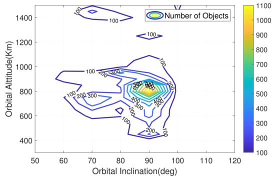
Figure 1.
Orbital altitude inclination distribution of LEO objects.
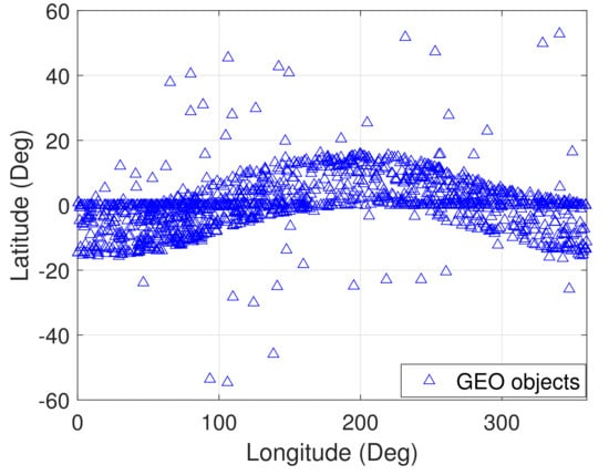
Figure 2.
Earth fixed longitude-latitude distribution of objects.
It is seen from Figure 1 that objects are spread in space with different spatial densities. The objects in the reference catalog are much more diverse in orbit type and size in the form of RCS. The object detection performance can be measured against a certain criterion or a combination of several criteria; for example, the performance can be expressed as a function of orbit altitude and size. Over a relatively short time period, a sensor can be operated to detect objects in a wide space domain and the actual detections can be compared to the predicted detections based on sensor parameters, with the resulting difference reflecting the accuracy of the sensor parameters.
2.2. A General Size Estimation Model Based on RCS Data
In addition to the position, object size plays an essential role in the performance evaluation, since it is used to compute the detection SNR or the object’s visual brightness. Unfortunately, the size information is uncertain because an object may have a complicated geometrical structure and varying attitude. The object size information published in the NORAD catalog is the equivalent RCS, which is an average of RCS sequences observed many times. RCS is the cross-sectional area of electromagnetic scattering of the object, which is a measure of the physical size to some extent. However, the relationship between the RCS, the physical size, the radar frequency band, and other factors is very complex [30], and the RCS cannot be directly converted to the object size or optical brightness. Example estimation models include the swelling fluctuation model [30] and the SEM model [31] of Lincoln Laboratory. Here, a generalized model to estimate physical size from RCS at different frequency bands is developed by the use of the RCS calculation formula for standard metal balls and the fluctuation characteristics of RCS.
In order to further fulfill the requirements of object detection performance evaluation in the real word, there are two problems that must be solved in developing the RCS-based size estimation model. One is to realize point-to-point size estimation from RCS, which should avoid effects from time-varying RCS fluctuation and complex coupling. The other is to form a monotonic mapping function between physical size and RCS by the use of the general electromagnetic scattering equivalency model and reduce the influence caused by object attitude and shape. It is expected that such a size estimate model should be valid and accurate for the performance evaluation. Here, a generalized model to estimate physical size from RCS at different frequency bands is developed by the use of the RCS calculation formula for a standard metal ball and the fluctuation characteristics of RCS.
For a metal conducting sphere with a diameter of D, its RCS, , can be expressed as a Mie series [30]:
where , is the wave number, is the radar wavelength, is the Bessel function of the first class of order n, is the Hankel function of order n, and is the Bessel function of the second class. The RCS computed from (1) may be approximated by a polynomial for a given and D:
where is a polynomial of order n, and are coefficients of the polynomial. The coefficients can be estimated by solving the following optimization equations where the theoretical RCS values are computed using (1) for various D and :
where is the second-order norm of a vector. In fact, the coefficients can be estimated by the least-squares method with the theoretical RCS, D, and as inputs. According to the relation between the RCS and wavelength, the scattering zone is usually divided into the optical zone and the Rayleigh zone , with the resonance zone in between, in which the RCS in the resonant zone fluctuates strongly with the object diameter and wavelength. There is no strict criterion to specify the RCS zones. As in [31], the diameter-to-wavelength ratios of 0.25 and 5.0 are used in this paper to form three RCS zones, and this results in a curve of the theoretical RCS as a function of the diameter-to-wavelength ratio, shown as red in Figure 3. It is seen that the RCS fluctuates in the resonance zone; thus, the mapping between the RCS and the diameter-to-wavelength ratio is not monotonic anymore, so the polynomial fitting of the theoretical RCS should be made separately for different zones. For the curve in Figure 3, it needs three polynomials, respectively, for three zones. For the optical or Rayleigh zone, a third-order polynomial will approximate the red curve in the specified zone. For the curve in the resonance zone, a second-order polynomial would be appropriate. Assuming the radar frequency f = 438.5 MHz, the polynomial fitting results are as follows, which are shown as blue in Figure 3:
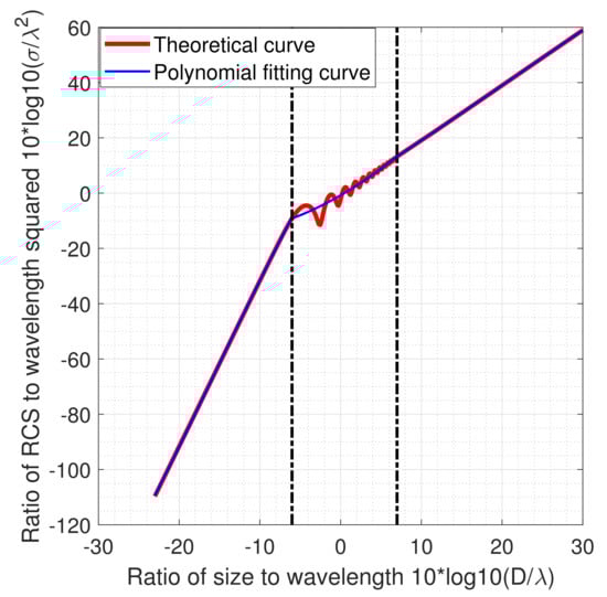
Figure 3.
Curves of theoretical RCS and polynomial fittings; radar frequency f = 438.5 MHz.
Now, with the fit polynomials, the physical size of the object D can be determined:
Using (5), one is able to determine a unique D corresponding to a given and wavelength . After obtaining the physical size D of an object, it should be possible to compute its RCS at other radar frequencies or to determine the visual magnitude of the object. As shown in Figure 4, the RCS values at radar frequencies of 438.5 MHz and 1.5 GHz are different.
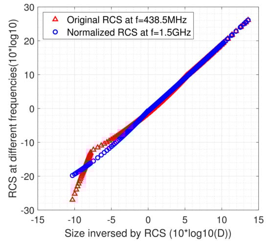
Figure 4.
Object RCS at two radar frequencies.
As can be seen from Figure 4, the size estimation model based on RCS data can depict quite well the numerical variation trends of the RCSs at the two different radar frequencies, and a simplified monotonic mapping relationship between the RCS and physical size can be formed. Based on the unified relationship between the RCS and object size, the SNR levels for optical or radar sensors can be evaluated.
3. A Hierarchy Scheme for Visibility Computation
The reference catalog of on-orbit objects and the model for estimating object physical size from the RCS data allow us to accurately evaluate the object detection performance of a sensor. For the evaluation, the visibility of an object with respect to the sensor at a specific time is the first to be computed (or predicted) using the position and size data of the object and the sensor’s detection parameters, such as the minimum SNR level. Because of the vast number of objects in the reference catalog, a fast and reliable visibility computation algorithm in which visible objects are not missed or falsely predicted visible is needed.
The visibility of an object with respect to a sensor is constrained by many factors. Typical constraints include distance, azimuth and azimuth ranges, searching beam, field of view (FOV), and minimum SNR. Imposing more constraints would slow the computation and thus affect the timeliness of the evaluation. A common practice is to first examine the constraint conditions point by point in a time window and then find the boundary of the visible time interval with the method of bisection [32], Although the algorithm is simple to implement, the time step length must be small enough to avoid missing visible time; as a result, the computation time is generally unacceptable.
An analysis of the spatial distribution of visible objects reveals that, for each individual object, the visible time intervals or visible orbit arcs with respect to a sensor are usually sparse and short in time duration. This suggests that the step-by-step algorithm can be improved by filtering out some invisible time periods during which the object will be invisible. This paper proposes an optimization approach to speed up the visibility computation. For this, an objective function subject to object visibility constraints is first derived; the function is then solved with a highly efficient numerical optimization method and the boundary of the visible regions is finally determined.
3.1. An Optimization Approach to Visible Time Interval Determination
The information needed for the visibility computation includes the object’s position and the sensor’s positional data and pointing detection parameters. The object position and velocity r and vector v are usually computed from cataloged elements, e.g., TLE. The sensor positional data includes the position vector R and velocity vector V at time t. A sensor can be ground-, sea-, or space-based, and operated in tracking or surveying mode; either way, the pointing direction of the sensor at time t is known. Given the above information, a few observables of the object relative to the sensor can be computed and each of these observables may be expressed as a function in the form of . For a space object to be detected by a sensor, each of relevant observables has to be within its respective visibility constraint region. For example, an object has to be within the FOV of a telescope, which may be specified by an azimuth range and an elevation range, such that the object will be possibly visible to the telescope. For each relevant observable, the visibility condition may be formulated as , where and represent the low and high boundaries of the visibility region, respectively. To determine whether the object is visible during a specified time window, is essential to determining whether there is any time interval in the window in which all the observables are within their preset constraint regions. The found object-visible time interval is denoted as , where and represent the starting and ending times, respectively.
For a particular visibility condition, one demands the following be true for the corresponding observable :
Equation (6) can be re-formulated to a zero-point problem:
The boundary value of Equation (7) is a zero point of equation
and of . In order to facilitate the optimization calculation, the solution to the zero-points of Equation (7) can be converted to a one-dimensional minimum optimization problem; that is, and are the solutions that minimize the following objective functions, respectively:
Equation (8) can be solved quickly using optimization algorithms such as the BRENT method [32], the golden section method [33], the or Goldstein method [34]. The solutions are , within the given time window . The solutions need to be evaluated as to whether the middle point meets the following conditions:
If Equation (9) holds for , then is a time interval during which the object is visible to the sensor. The observable is usually not monotonic in a long time window and solving (8) results in multiple zero points and . One option to ease this problem is to divide the whole time window into a few sub-windows in each of which the observable becomes monotonic. Given the sensor, operation mode, space object, and the observable, such sub-windows can be easily determined by a simple analysis of the observable’s monotonicity. The length of such sub-windows is usually quite long. Assume that, for a ground radar, the maximum distance and minimum elevation for an object to be visible to the radar are 6000 km and 30°, respectively. By analyzing the curves of the objective functions for the distance and elevation of the object with NORAD ID 00005 over a time window of 24 h, as shown in Figure 5, the time sub-windows are easily determined.
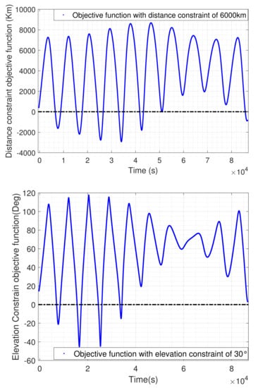
Figure 5.
Objective functions for the distance (up) and elevation (down) constraints.
It is seen from Figure 5 that, for either the distance or elevation, a sub-window is about half of the orbital period. In Figure 5, the object-visible time intervals are where the objective functions are less than zero. For each sub-window, the derivatives of the objective function with respect to the constraint observable at the two end points are computed and if the signs of the two derivatives are different, the sub-window is further divided into shorter sub-windows. In this way, the zero points of (8) can be quickly solved for the final sub-windows and the boundaries of the visible time intervals are eventually obtained.
3.2. Hierarchy Scheme for Multi-Constraint Visibility Computation
In the above, the visible time interval subject to one constraint is determined by solving the optimization problem of Equation (8). For an object to be detected by a sensor, there are multiple constraint observables, each of which must make Equation (6) true. That is, for each observable, there can be one or more visible time intervals. The visible time intervals determined for all constraints may form some overlap intervals, which are then the final visible time intervals. This visibility computation method is termed the overlapping technique, because each of the final visible time intervals is an overlapped interval during which all the visibility conditions are held, whereas each individual condition is independently applied to determine the corresponding time intervals.
A practical problem with the overlapping approach is the potential heavy computation burden when the visibility computation is required for a large number of space objects and multiple sensors. It is necessary to speed up the computation, and this is possible since the observable orbital arcs of space objects by a space surveillance sensor are sparse and short in time duration, usually only a few minutes or less. In fact, when the visible time intervals have been determined with one or more constraints, only these intervals need to be considered as to whether they are also visible time intervals under the next constraint. The most likely outcome is that the lesser and shorter visible intervals are subject to all applied constraints. This hierarchy time interval determination scheme can be repeated for the remaining constraints and as a result, the efficiency of the visibility computation can be greatly improved.
The hierarchy scheme is easy to implement, but the constraint priority is needed to determine in what order the constraints should be sequentially applied to determine the visible time intervals. The priority can be determined according to the lengths of the visible time intervals under each constraint. The first constraint is the one that results in the longest interval duration, the second constraint is the one with the second-longest duration, and so on. For commonly used radar or optical sensors, the distance constraint is clearly the most prioritized constraint, followed by the elevation, azimuth, FOV, SNR, and illumination constraints, all of which have no preferred priority order.
A comparison of the computing times with the overlapping technique and hierarchy scheme was made for a simulated ground-based radar. The radar was assumed to be able to detect an object at a distance of 6000 km. Therefore, the first constraint is that the distance is less than 6000 km. Other visibility constraints are that the elevation is higher than 30°, the azimuth is in the 120°–240° range, and the SNR is larger than 12.6 dB. The visible time intervals were computed with the two techniques for an object of RCS 0.1 m at an orbital altitude of 600 km, and the determined visible arcs/time intervals and computing times are given in Table 1.

Table 1.
Comparison of visible time interval computation.
It can be seen from Table 1 that using the overlapping technique will result in a total of 172 visible arcs/time intervals with a computation time of 14.6 s. In contrast, the computation time using the hierarchy scheme is reduced by 36% because 23% of the arcs are ignored in the sequential constraints. Such an improvement in computation efficiency is very valuable for visibility computation of a large number of space objects.
4. Detection Performance Analysis Based on Data Point Matching
After the visibility prediction for objects in the reference catalog, it is now feasible to accurately analyze the nominal detection parameters of the sensor. A straightforward way is to first compare the observed arcs to the predicted arcs and then use differences to analyze the detection performance from different perspectives.
4.1. Matching of Predicted and Observed Data Points
The correctness of the match between the observed and predicted data is affected by the errors existing in both types of data, the threshold, and the used matching method. The predicted data is based on relatively accurate orbital elements of an object of known identity, whereas the observed data is mostly from a short orbit arc from which only inaccurate initial orbit elements can be estimated. Therefore, it is inappropriate to perform the data matching using the orbit elements, but the estimated initial orbit elements may be used to screen out some predicted arcs that are impossible to match to an observed arc.
After the preliminary screening, point-by-point differences (or residuals) between the observed and predicted data are computed. Assuming that the observations of an object are collected by a sensor at N time epochs, and given the set of TLE (or precise ephemeris, if available) of an object, the positions at the observation epochs can be computed with the SGP4/SDP4 algorithm (or associated algorithm) and thus the corresponding “observations” (or predictions) in the form of the distance between the object and the sensor, and the azimuth/elevation or right ascension/declination of the object with respect to the sensor, can be computed. Depending on the sensor type, there could be one or more sequences of observation residuals for the observed arc. For example, given a radar sensor, we could have three sequences in the azimuth, elevation, and range, respectively. A residual sequence can be denoted as . The residual sequences contain comprehensive information about the observations and their corresponding predictions, and can be used to form some parameters, denoted as M, which in turn are used to judge whether the observed arc is correlated to the predicted arc.
From a residual sequence, two types of parameters, statistical and physical, can be derived. Typical statistical parameters are the mean of the residuals , the median of the residuals , the standard deviation of the residuals , and the of the residuals . On the other hand, a residual sequence may be modeled by a linear function of time . In this case, represents the systematic bias and represents the change rate of the residuals, which has clear physical meanings. For instance, when the radar range residuals are fit to the linear function, is then the systematic bias between the measured and predicted ranges, and is the change rate of the range residuals. Additional parameters may be defined for some unique detection scenarios.
A match between an observed and a predicted arc could be declared if all or some of parameters M are less than their respective threshold . Given a residual sequence , the match equation can be expressed as, for example:
where and are the thresholds for the and change rate of the residuals, respectively. Depending on whether the sensor is optical or radar, there could be two or three match equations, each of which should hold to declare a match between an observed and a predicted orbit arc.
The threshold values should be determined considering the orbit prediction error, observation error, and other factors. Small thresholds reduce the mismatch probability, but increase missed matches. Therefore, optimal thresholds are desired. They can be found following two rules: the thresholds result in a less than 5% mismatch probability; and an increase of 10% in the thresholds increases correct matches by less than 1%.
4.2. Performance Evaluation Procedure
We have now discussed the three critical aspects in sensor detection performance evaluation using an on-orbit object catalog, i.e., the estimation of object size from its RCS, the computation of the visible time periods, and the matching of the observed and predicted data. The final aspect is to determine features that most concern engineering perspectives.
In this paper, we focus on the two important features regarding the detection performance of a sensor: one is the spatial-temporal coverage of the sensor and the other is its actual object detection ability. Given appropriate definitions of these two features and the corresponding indices, which can be computed, the detection performance can now be evaluated with the procedure shown in Figure 6. We propose using detection probability, which is defined as the ratio of the number of both observed and matched arcs to the number of predicted arcs, to measure performance. The inputs include the TLE catalog, the sensor parameters, and the observed data. The thresholds for the data match also need to be set.
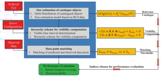
Figure 6.
Schematic diagram of the proposed performance evaluation procedure.
Note that for each of these two features, a few qualitatively computable indices that represent the most required performance are needed. They will be defined along with the examples presented below.
4.3. Detection Performance Evaluation Examples
In the following section, the spatial-temporal detection coverage and the actual detection ability of two sensors are evaluated with the proposed approach. One sensor is a ground-based wide-area space surveillance radar and the other is a space-based optical telescope. The radar is assumed to be pointing upwards with space coverage from the zenith downward to 30° of elevation. It is designed to detect LEO objects. The space-based optical telescope takes the Space Based Space Surveillance (SBSS) satellite as its prototype. It is on a near-circular sun-synchronous orbit, points away from the Sun, and aims to survey objects in the full GEO region.
We may point out that, for each sensor, although the duration of data used in the analyses is only a few days, it should be appropriate to demonstrate the effectiveness of the proposed evaluation approach
4.3.1. Spatial-Temporal Coverage
The indices for measuring the spatial-temporal coverage are the spatial coverage, temporal stability, and observation timeliness. The three indices are used to examine whether there is any discontinuity in the detection operation and whether there is any space area where the detection is less likely to be successful, all the most concerning factors for sensor users.
The space coverage in this paper is concerned with the detection probability in the intended space area. If the space area covered by the sensor is large, the space can be further divided into multiple regions of equal area. Figure 7 and Figure 8 shows the simulated radar’s detection performance over a time span of 24 h in the covered space. In the Figure 7, the visible objects, marked as blue circles, are the observed objects, and the invisible objects marked as red triangle are the predicted, but not observed objects. They are shown with respect to the distance between the radar and object, and the space angle, which is the zenith angle of the object. In order to differentiate the location of an object, the space angle is set positive if the object is in the east part of the sky, and negative if it is in the west.
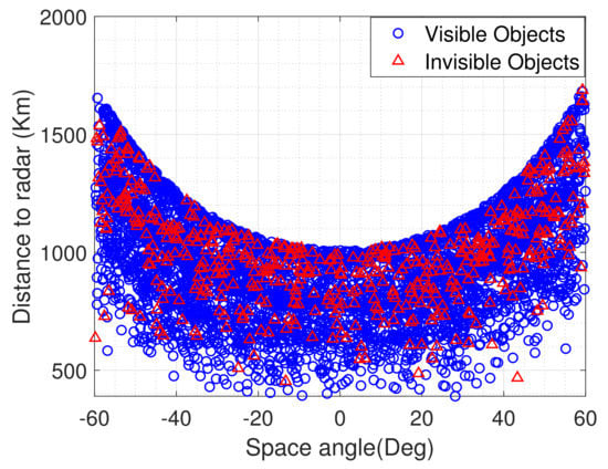
Figure 7.
Detection performance of the simulated radar in the covered space.
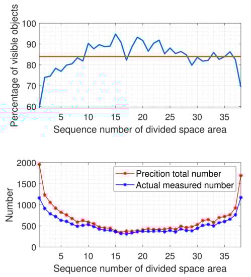
Figure 8.
Detection performance of the simulated radar in the covered space.
The simulated ground-based wide-area surveillance radar has a very good detection performance in the intended space which extends from the zenith to the low boundary of the radar beam at the elevation of 30°, as seen from the Figure 8. The number of invisible objects is only a fraction of the visible objects. In terms of the detection probability defined above, it is generally above 80% for most of the covered space, as seen in the top figure. Clearly, the number of observed objects is less than that of the predicted ones, suggesting there may be some issues in the sensor and/or the evaluation.
The radar has a wide-area FOV. When the FOV is divided into 38 regions of equal beam width, the detection probability in different regions, shown in the top figure, is uneven. The detection probability on the fence edge is relatively low, indicating that the achieved detection capability of the sensor in parts of its intended space is lower than expected. Because this detection probability is evaluated based on high-precision predictions and matched observation arcs, shown respectively as red and blue marks in the bottom figure, its reliability is undoubtfully much higher than that from infield and outfield static tests. Importantly, the evaluation has uncovered the areas in the radar fence where the detection performance is weak, which would help identify potential defects in the sensor’s design, manufacture, deployment or operation. In fact, this is one of the reasons to carry out the routine performance evaluation.
Next, the temporal stability, which describes the stability of a sensor’s detection probability over time is analyzed. A small fluctuation in the detection probability over time indicates the sensor has steady detection performance. Figure 9 shows the hourly detection probability of the simulated radar over a time span of 72 h.
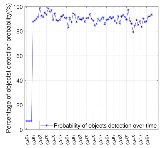
Figure 9.
Temporal stability of the detection probability of the simulated radar.
As can be seen from Figure 9, the overall detection probability of the radar over time is relatively stable at over 80%, with the peak at almost 100%. However, the performance appears to decline slowly with time even in the short span of 72 h, which could be a concern to be monitored further. A very disturbing issue is that the radar does not perform well in the early stage of the operation, during which the detection probability is very low. In most cases, slight fluctuations in the detection probability over time would be hard to notice without a detailed and continuous temporal stability evaluation against a reference catalog. It helps to obtain an accurate assessment of the sensor’s detection performance stability in each time interval, along with the long-term operation capability.
Another important performance index is observation timeliness, which describes the time interval between two consecutive observed orbit arcs for an object. A short interval indicates that more orbital arcs are observed, which is necessary for achieving high precision orbit determination of an object. By comparing the differences between the predicted intervals and the actual intervals, a sensor’s operation strategy can be optimized. Figure 10 shows the distribution of the time intervals for GEO objects observed by the simulated space-based optical telescope.
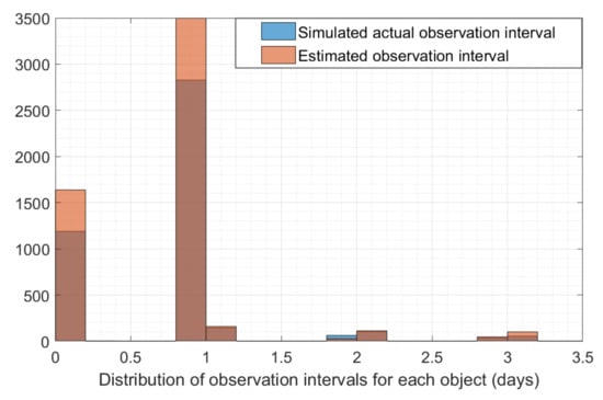
Figure 10.
Observation timeliness of GEO objects by the simulated space-based optical telescope.
It can be seen from Figure 10 that the time interval for most GEO objects is about one day, as expected with the designed operation mode. This is consistent with the orbital period of GEO objects. It can also be found that a large portion of GEO objects have much shorter observation intervals of only 2 to 3 h, which shows that the designed operation mode enables the sensor to observe these GEO objects twice in a short time, and thus the observation timeliness is quite impressive for these objects. However, for some objects, the time intervals are 2 or even 3 days. Further analysis reveals that these objects are mostly on orbits of relatively large inclination, indicating that the designed operation mode is inappropriate for GEO objects of high inclination. On the whole, the predicted time intervals generally agreed well with the actual time intervals, with the number of the former being slightly more than that of the latter, indicating that the actual performance in terms of the observation time interval is only slightly worse than that expected. The analysis provides an accurate description of the GEO objects’ observation timeliness achieved with the designed operation mode of the telescope, and an enhancement may be made by refining the operation mode.
4.3.2. Detection Ability
In this paper, the object detection ability of a sensor, depending on whether it is a radar or a telescope, is measured by one of two indices. Radar sensors use the SNR-dependent detection probability and telescopes use the object size-related detection probability. The former describes a radar’s signal acquisition capability in terms of SNR and the latter describes the size of the objects detectable by a telescope.
The SNR-dependent object detection probability is also defined as the ratio of the number of detected objects to the number of predicted objects. It is different from the commonly used signal detection probability [35]. The SNR-dependent detection probability describes a sensor’s object detection ability with respect to the variations of the geometrical shape and attitude (tumbling) of space objects. Figure 11 shows the SNR-dependent object detection probability of the simulated radar as a function of the SNR.
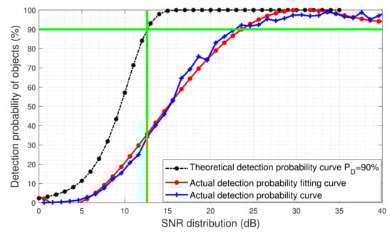
Figure 11.
SNR-dependent object detection probability of the simulated radar.
It can be seen from Figure 11 that when the SNR is higher than 12.6 dB, the theoretical detection probability will be above 90%. However, the actual detection probability will only reach 90% when the SNR is higher than 23 dB. This is most likely caused by the uncertainty in the estimated object’s RCS. By comparing the detection probability curve of objects with the Swerling model of RCS fluctuation [30], it can be found that the RCS fluctuation of detected space objects is similar to the RCS fluctuation model of Swerling Type I for slow objects; these objects are usually difficult to detect. Because the geometrical structure and attitude of space object are very likely unknown, the assumed object RCS will be different from the actual RCS; therefore, it is understandable that the actual SNR-dependent detection probability is different from the theoretical one. The difference can only be obtained by accurately evaluating the actual SNR-dependent detection probability for on-orbit objects.
The size-related object detection probability is more intuitive for describing an optical sensor’s object detection ability. As presented earlier, object size is estimated from RCS, which itself has unknown uncertainty, and thus the resultant size has uncertainty. Consequentially, the size-related detection probability curve is less smooth. Considering the simulated space-based telescope, the size-related detection probability for GEO objects is shown as a function of object size in Figure 12.
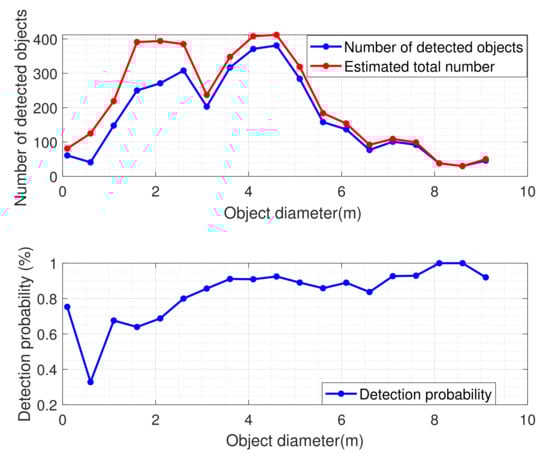
Figure 12.
Size-related GEO object detection probability of the simulated space-based telescope.
It is seen in Figure 12 that for GEO objects large than 3.5 m in diameter the telescope’s detection probability is basically above 90%. However, as the object size decreases, the detection probability declines rapidly. The size-related detection probability curve is also not as stable or smooth as the SNR-dependent curve. However, it can accurately describe the telescope’s GEO object detection ability as a function of object size, which is of great importance for sensor design and manufacture.
5. Conclusions
For designers, manufacturers, and operators of space object surveillance sensors, realized performance in space object detection in the real word should be the most important concern, and evaluation of this concern can not be achieved by simulations. Although there are evaluations at various phases of sensor development, including tests on performance during the deployment phase using a limited number of calibration satellites, these are not sufficient. Therefore, an implementable and reliable evaluation procedure is desirable. This paper proposes to evaluate object detection performance by analyzing real data collected in the operational environment using cataloged on-orbit objects as reference. Performance should be qualitatively measured; as such, detection probability is proposed as the key index, and it can be used to describe important performance features such as space coverage and temporal stability.
The evaluation requires size and visibility information on space objects, the accuracy of which affects the evaluation reliability. In this paper, a size estimation model using the RCS data in the TLE catalog is presented. To ease the computation burden when determining the visibility of vast number of space objects, a hierarchy scheme was developed that is able to compute the visibility quickly and accurately. With the available size, RCS, and visibility data of reference objects, the space object detection performances of two simulated sensors—a ground-based wide-area surveillance radar for LEO objects and a space-based telescope surveying GEO objects—were evaluated, during which a number of performance indices were defined and computed. For the simulated radar sensor, it was found that the detection probability at the radar fence edge is significantly lower than at other parts of the fence. It was also found that the detection probability at the early stage of detection operation is much lower than that at a later time. For the optical sensor observing objects in the GEO orbit region, detection ability was weak for objects of small sizes. Generally, the computed detection probability demonstrates that achieved detection performance is mostly inferior to expected performance.
The proposed procedure can be used routinely and is applicable to any space surveillance sensor or sensor system. Detection performance can thus be monitored to identify issues and to implement necessary modifications to maintain the required detection performance. If differences between evaluated and expected performance persist, they may be very useful to help identify defects in the sensors or data processing algorithms that potentially exist in the various phases of design, manufacture, deployment, and operation.
In future implementations of the proposed method, causes for the difference between the designed and realized performance of an individual sensor should be a focus of study. Furthermore, the collective performance of a sensor network, such as its capability for object cataloging, should be assessed.
Author Contributions
Methodology, J.H.; software, J.H.; validation, X.L. and B.L.; formal analysis, X.L.; investigation, B.L.; writing—original draft preparation, J.H., H.L. and J.S.; writing—review and editing, H.L. and J.S.; visualization, X.L. and B.L. All authors have read and agreed to the published version of the manuscript.
Funding
This research was funded by the National Natural Science Foundation of China (Grant No. 41874035) and the Natural Science Foundation of Hubei Province, China (Grant No. 2020CFB396).
Institutional Review Board Statement
Not applicable.
Informed Consent Statement
Not applicable.
Data Availability Statement
Not applicable.
Conflicts of Interest
The authors declare no conflict of interest.
References
- Sridharan, R.; Pensa, A.F. Us space surveillance network capabilities. In Image Intensifiers and Applications, and Characteristics and Consequences of Space Debris and Near-Earth Objects: San Diego, CA, USA, 23 July 1998; SPIE Proceedings Series; SPIE: San Diego, CA, USA, 1998; Volume 3434, pp. 88–100. [Google Scholar]
- Yaglioglu, B.; Utku, A.; Yilmaz, O.; Ozdemir, B.G. Surveillance of space: An overview and a vision for Turkey’s roadmap. In Proceedings of the 2013 6th International Conference on Recent Advances in Space Technologies (RAST), Istanbul, Turkey, 12–14 June 2013; pp. 1041–1046. [Google Scholar] [CrossRef]
- Albon, C. Space Fence IOC delayed seven months due to early schedule slips. Inside Air Force 2017, 28, 1–7. [Google Scholar]
- Fonder, G.; Hughes, M.; Dickson, M.; Schoenfeld, M.; Gardner, J. Space Fence Radar Overview. In Proceedings of the 2019 International Applied Computational Electromagnetics Society Symposium (ACES), Miami, FL, USA, 14–18 April 2019; pp. 1–2. [Google Scholar]
- Ruprecht, J.D.; Stuart, J.S.; Woods, D.F.; Shah, R.Y. Detecting small asteroids with the Space Surveillance Telescope. Icarus 2014, 239, 253–259. [Google Scholar] [CrossRef]
- Richardson, D. USAF plans follow-on SBSS satellite. In Jane’s Missiles and Rockets; Jane’s Information Group Ltd.: Coulsdon, UK, 2010; p. 16. [Google Scholar]
- Punjani, S.; Bogstie, H.; Grady, J.; Hogan, M.; Moomey, E.; Zaza, R.; Berenberg, L. ORS-5 System Acquisition Successes and Regrets. Technical Report. 2018. Available online: ORS-5SystemAcquisitionSuccessesRegrets-ShahnazPunjani.pdf (accessed on 10 January 2022).
- Th, M.; Eglizeaud, J.; Bouchard, J. GRAVES: The new French system for space surveillance. In Proceedings of the 4th European Conference on Space Debris, Darmstadt, Germany, 18–20 August 2005; Volume 587, p. 31. [Google Scholar]
- Klinkrad, H. Monitoring Space–Efforts Made by European Countries; International Colloquium on Europe and Space Debris: Darmstadt, Germany, 2002; Volume 51. [Google Scholar]
- Huang, J.; Hu, W.; Ghogho, M.; Xin, Q.; Du, X.; Guo, W. A novel signal processing approach for LEO space debris based on a fence-type space surveillance radar system. Adv. Space Res. 2012, 50, 1462–1472. [Google Scholar] [CrossRef]
- Saaty, R.W. The analytic hierarchy process—What it is and how it is used. Math. Model. 1987, 9, 161–176. [Google Scholar] [CrossRef]
- Rodriguez, R. Models, methods, concepts and applications of the analytic hierarchy process. Interfaces 2002, 32, 93. [Google Scholar]
- Levis, A.H. Modeling and Measuring Effectiveness of C3 Systems; Technical Report; Massachusetts Inst of Tech Cambridge Lab for Information and Decision Systems: Cambridge, MA, USA, 1986. [Google Scholar]
- Wold, S.; Esbensen, K.; Geladi, P. Principal component analysis. Chemom. Intell. Lab. Syst. 1987, 2, 37–52. [Google Scholar] [CrossRef]
- Zhong, M.; Guo, J.; Yang, Z. On Real Time Performance Evaluation of the Inertial Sensors for INS/GPS Integrated Systems. IEEE Sens. J. 2016, 16, 6652–6661. [Google Scholar] [CrossRef]
- Otegui, J.; Bahillo, A.; Lopetegi, I.; Díez, L.E. Performance Evaluation of Different Grade IMUs for Diagnosis Applications in Land Vehicular Multi-Sensor Architectures. IEEE Sens. J. 2021, 21, 2658–2668. [Google Scholar] [CrossRef]
- Donath, T.; Schildknecht, T.; Brousse, P.; Laycock, J.; Michal, T.; Ameline, P.; Leushacke, L. Proposal for a European space surveillance system. In Proceedings of the 4th European Conference on Space Debris, Darmstadt, Germany, 18–20 April 2005; ESA SP-587. ESA/ESOC: Darmstadt, Germany, 2005; Volume 587, p. 31. [Google Scholar]
- Donath, T.; Schildknecht, T.; Martinot, V.; Del Monte, L. Possible European systems for space situational awareness. Acta Astronaut. 2010, 66, 1378–1387. [Google Scholar] [CrossRef]
- Flohrer, T.; Schildknecht, T.; Musci, R.; Stöveken, E. Performance estimation for GEO space surveillance. Adv. Space Res. 2005, 35, 1226–1235. [Google Scholar] [CrossRef]
- Flohrer, T.; Schildknecht, T.; Musci, R. Proposed strategies for optical observations in a future European Space Surveillance network. Adv. Space Res. 2008, 41, 1010–1021. [Google Scholar] [CrossRef]
- Schildknecht, T.; Flohrer, T.; Musci, R. Optical observations in a proposed European Space Surveillance network. In Proceedings of the 6th US Russian Space Surveillance Workshop, Central Astronomical Observatory at Pulkovo of Russian Academy of Sciences, St. Petersburg, Russia, 22–26 August 2005; pp. 9–21. [Google Scholar]
- Olmedo, E.; Nomen, J.; Sánchez-Ortiz, N.; Belló-Mora, M. Cataloguing capability of objects in the GEO ring. In Proceedings of the 60th International Astronautical Congress, Daejeon, Korea, 12–16 October 2009; Volume 5, pp. 12–16, Paper IAC-09-A6. [Google Scholar]
- Olmedo, E.; Sánchez-Ortiz, N. Space debris cataloguing capabilities of some proposed architectures for the future European Space Situational Awareness System. Mon. Not. R. Astron. Soc. 2010, 403, 253–268. [Google Scholar] [CrossRef][Green Version]
- Früh, C.; Schildknecht, T.; Hinze, A.; Reber, M. Optical observation campaign in the framework of the ESA space surveillance system precursor services. In Proceedings of the European Space Surveillance Conference, Madrid, Spain, 7–9 June 2011. [Google Scholar]
- Utzmann, J.; Wagner, A.; Blanchet, G.; Assémat, F.; Vial, S.; Dehecq, B.; Sánchez, J.F.; Espinosa, J.R.G.; Maté, A.Á.; Bartsch, G.; et al. Architectural design for a European SST system. In Proceedings of the 6th European Conference on Space Debris, Darmstadt, Germany, 22–25 April 2013. [Google Scholar]
- Hu, J.; Hu, S.; Liu, J.; Chen, X. Simulation Analysis of Space Debris Observation Capability of Multi-Optoelectronic Equipment. Acta Opt. Sin. 2020, 40, 1504002. (In Chinese) [Google Scholar]
- Butkus, A.; Roe, K.; Mitchell, B.; Payne, T. Space surveillance network and analysis model (SSNAM) performance improvements. In Proceedings of the 2007 DoD High Performance Computing Modernization Program Users Group Conference, Pittsburgh, PA, USA, 18–21 June 2007; pp. 469–473. [Google Scholar]
- Krag, H.; Beltrami-Karlezi, P.; Bendisch, J.; Klinkrad, H.; Rex, D.; Rosebrock, J.; Schildknecht, T. PROOF—The extension of esa’s MASTER Model to predict debris detections. Acta Astronaut. 2000, 47, 687–697. [Google Scholar] [CrossRef]
- Vallado, D.; Crawford, P. SGP4 orbit determination. In Proceedings of the AIAA/AAS Astrodynamics Specialist Conference and Exhibit, Honolulu, HI, USA, 18–21 August 2008; p. 6770. [Google Scholar]
- Barton, D.K. Radar System Analysis and Modeling; Artech House: Dedham, MA, USA, 2004. [Google Scholar]
- Lambour, R.; Rajan, N.; Morgan, T.; Kupiec, I.; Stansbery, E. Assessment of orbital debris size estimation from radar cross-section measurements. Adv. Space Res. 2004, 34, 1013–1020. [Google Scholar] [CrossRef]
- Brent, R.P. Algorithms for Minimization without Derivatives; Courier Corporation: North Chelmsford, MA, USA, 2013. [Google Scholar]
- Bandler, J.W. Optimization methods for computer-aided design. IEEE Trans. Microw. Theory Tech. 1969, 17, 533–552. [Google Scholar] [CrossRef]
- Venkataraman, P. Applied Optimization with MATLAB Programming; John Wiley & Sonsa: Hoboken, NJ, USA, 2009. [Google Scholar]
- Ender, J.; Leushacke, L.; Brenner, A.; Wilden, H. Radar techniques for space situational awareness. In Proceedings of the 2011 12th International Radar Symposium (IRS), Leipzig, Germany, 7–9 September2011; pp. 21–26. [Google Scholar]


Publisher’s Note: MDPI stays neutral with regard to jurisdictional claims in published maps and institutional affiliations. |
© 2022 by the authors. Licensee MDPI, Basel, Switzerland. This article is an open access article distributed under the terms and conditions of the Creative Commons Attribution (CC BY) license (https://creativecommons.org/licenses/by/4.0/).