Article

Using Unoccupied Aerial Vehicles (UAVs) to Map Seagrass Cover from Sentinel-2 Imagery

1
National Oceanography Centre, European Way, Southampton SO14 3ZH, UK
2
Ocean and Earth Sciences, University of Southampton, Southampton SO14 3ZH, UK
3
Green Rebel Marine, Crosshaven, P43 EV21 Cork, Ireland
4
Turneffe Atoll Sustainability Association, 1216 Blue Marlin Blvd, Belize City, Belize
5
UK Centre for Ecology and Hydrology, Bangor LL57 2UW, UK
6
Coastal Zone Management Authority and Institute, Princess Margaret Drive, Belize City, Belize
7
NORCE, Norwegian Research Centre AS, Bjerknes Centre for Climate Research, 5007 Bergen, Norway
*
Author to whom correspondence should be addressed.
Remote Sens. 2022, 14(3), 477; https://doi.org/10.3390/rs14030477
Submission received: 7 December 2021 / Revised: 13 January 2022 / Accepted: 17 January 2022 / Published: 20 January 2022

Abstract

:
Seagrass habitats are ecologically valuable and play an important role in sequestering and storing carbon. There is, thus, a need to estimate seagrass percentage cover in diverse environments in support of climate change mitigation, marine spatial planning and coastal zone management. In situ approaches are accurate but time-consuming, expensive and may not represent the larger spatial units collected by satellite imaging. Hence, there is a need for a consistent methodology that uses accurate point-based field surveys to deliver high-quality mapping of percentage seagrass cover at large spatial scales. Here, we develop a three-step approach that combines in situ (quadrats), aerial (unoccupied aerial vehicle—UAV) and satellite data to map percentage seagrass cover at Turneffe Atoll, Belize, the largest atoll in the northern hemisphere. First, the optical bands of four UAV images were used to calculate seagrass cover, in combination with in situ data. The seagrass cover calculated from the UAV was then used to develop training and validation datasets to estimate seagrass cover in Sentinel-2 pixels. Next, non-seagrass areas were identified in the Sentinel-2 data and removed by object-based classification, followed by a pixel-based regression to calculate seagrass percentage cover. Using this approach, percentage seagrass cover was mapped using UAVs (R2 = 0.91 between observed and mapped distributions) and using Sentinel-2 data (R2 = 0.73). This work provides the first openly available and explorable map of seagrass percentage cover across Turneffe Atoll, where we estimate approximately 242 km2 of seagrass above 10% cover is located. We estimate that this approach offers 30 times more data for training satellite data than traditional methods, therefore presenting a substantial reduction in cost-per-point for data. Furthermore, the increase in data helps deliver a high-quality seagrass cover map, suitable for resolving trends of deteriorating, stable or recovering seagrass environments at 10 m2 resolution to underpin evidence-based management and conservation of seagrass.

1. Introduction

Seagrasses are marine angiosperms that form meadows in shallow inter- and sub-tidal areas [1]. They play crucial roles in coastal tropical, sub-tropical and temperate ecosystems [2], covering approximately 160,000 km2 around the world [3]. Seagrasses provide a range of provisioning, regulating and cultural ecosystem services [4] that contribute to human welfare, particularly coastal populations [5]. They offer nursery habitats [6], food sources and shelter to various marine organisms, thus supporting biodiversity, endangered marine species and an estimated 20% of global fisheries production [7]. These habitats are typically associated with high accumulation rates of organic matter and build rich sedimentary carbon stores, so-called ‘blue carbon’, which removes CO2 from the atmosphere [8]. Also known as habitat builders, seagrass meadows help compensate for sea-level rise and reduce the flow, turbulence and wave action in their immediate vicinity, which results in increased sedimentation rates and stabilises the sediment [9]. Despite providing these services, vast reductions in seagrass meadow extent have occurred due to a variety of stressors, including terrestrial inputs [10], mechanical damage and clearing [11], increasing sea surface temperature and sea-level rise [12]. The spatial distribution of seagrass is affected by a combination of these stressors and other factors such as topography, hydrodynamics and water quality [13], which change the level of energy, either light or kinetic, within its vicinity. Thus, monitoring seagrass extent and cover, and their changes over time, is vital to identify threats and underpin evidence-based management strategies to conserve and restore them.
Seagrass monitoring is dependent on habitat mapping and the observation of biophysical properties at the appropriate scale [1]. Loss of seagrass cover may flag the potential influence of stressors, whereas gains may help identify the management strategy’s effectiveness. Data on biophysical properties such as aboveground biomass and leaf area index can be used as proxies for ecosystem services such as wave attenuation [14]. Assessing the longevity of seagrass meadows indicates the effectiveness with which certain ecosystem services are provided, such as the stabilisation of sedimentary carbon stocks. [15]. Despite its importance to coastal management, seagrass monitoring is hampered by the methodological limitations of the current mapping techniques [16].
An array of techniques has been applied to map seagrass, including satellites, acoustics, unoccupied aerial vehicles (UAVs) and field surveys, each capturing different spatial and thematic details [8]. Open-source global satellite data are readily available and offer a low-cost option for users compared with field sampling, acoustics or airborne scanners [17]. Commercial satellites collect highly spatially resolved data, but this has a high purchase cost. The open availability of median-resolution satellites (pixel size 10–30 m), such as Landsat (30 m), has resulted in their widespread use in seagrass mapping. Since 2016, the improved temporal and spatial coverage provided by Sentinel-2 (10 m) has led to its dominance in the more recent seagrass mapping literature [18].
There are several parameters of interest regarding seagrass that can theoretically be derived from remote sensing observations. These include presence/absence, percentage cover and species composition. A consensus has yet to be reached regarding the effectiveness of satellite data for mapping seagrass percentage cover. Sentinel-2 data have been utilised successfully for presence/absence seagrass mapping, with accuracies of over 90% [19,20,21]. However, considerably lower accuracies have been reported when mapping percentage cover by Fauzan [22] and Kovacs [23] of between 54 and 62%, and by Phinn [2] of less than 45% when using Landsat 5 data, CASI and Quickbird images. Direct comparisons of the performances of the satellite-based mapping approaches used in these studies are confounded by a lack of consistency in seagrass class groupings and the absence of the consideration of water depth within the input bands, which is crucial due to the inherent attenuation of light in water.
Despite recognition of the utility of quantitative, regression-based approaches to model continuous percentage seagrass cover [2], to our knowledge, there have been few attempts to do so. Of these, the study by Fauzan [22] was limited by sparse underpinning data and a dark-object atmospheric correction method that was handicapped by the inaccurate assumption of a uniform atmosphere and surface reflection. Highly accurate seagrass cover estimates have been recorded by Zoffoli [24] using the Normalised Difference Vegetation Index on intertidal seagrass. However, intertidal seagrass mapping is less challenging than subtidal as the reflectance is less disturbed by the physical properties of the water column.
To calibrate satellite data, in situ estimates of seagrass cover, typically made from randomly placed quadrats within the pixel area, are extrapolated to the whole pixel [24,25]. Thereby, estimates of seagrass cover derived from within the quadrat are assumed to represent the entire area of the pixel or seagrass patch. This assumption is made despite quadrats sampling a fraction of the area covered by one satellite pixel and when seagrass cover is often heterogeneous within a pixel [26]. To compensate for this, it is optimal to include as much validation data as possible. However, field surveys, particularly in submerged habitats, are often difficult to access and can be labour- and resource-intensive, limiting the number of sites they include.
Imagery collected by camera-equipped UAVs vastly exceeds the resolution of open-source satellite imagery and thus has emergent applications for such fine-scale mapping [27]. Seagrass biophysical properties can be mapped at various levels of detail, from the individual shoot up to the whole ecosystem level [2], and require datasets appropriate to the target feature’s scale. Specifically, centimetre-resolved UAV imagery can capture information to the shoot level [28,29,30]. Few studies have mapped seagrass percentage cover using UAVs, but highly accurate estimates have been achieved when describing seagrass cover in two density classes [31]. Provided the UAV imagery is free from glint and wave artefacts, it is possible to accurately estimate seagrass coverage within a satellite-sized pixel by averaging pixels at a higher resolution. By combining field surveys (for ground-truthing) with UAV and satellite data, there is an opportunity to retrieve more accurate values of seagrass cover within a satellite pixel whilst increasing the quantity and spread of data available for training and validation.
In this study, we derive a three-part classification to estimate continuous seagrass percentage cover from Sentinel-2 imagery using UAVs. By combining UAV and Sentinel-2 data, we show how high-resolution UAV imagery can be used to summarise seagrass cover within a Sentinel-2 pixel to train and validate a model at a large scale. This study presents the first map of seagrass percentage cover at Turneffe Atoll, the largest marine reserve in Belize and a global biodiversity hotspot [32].

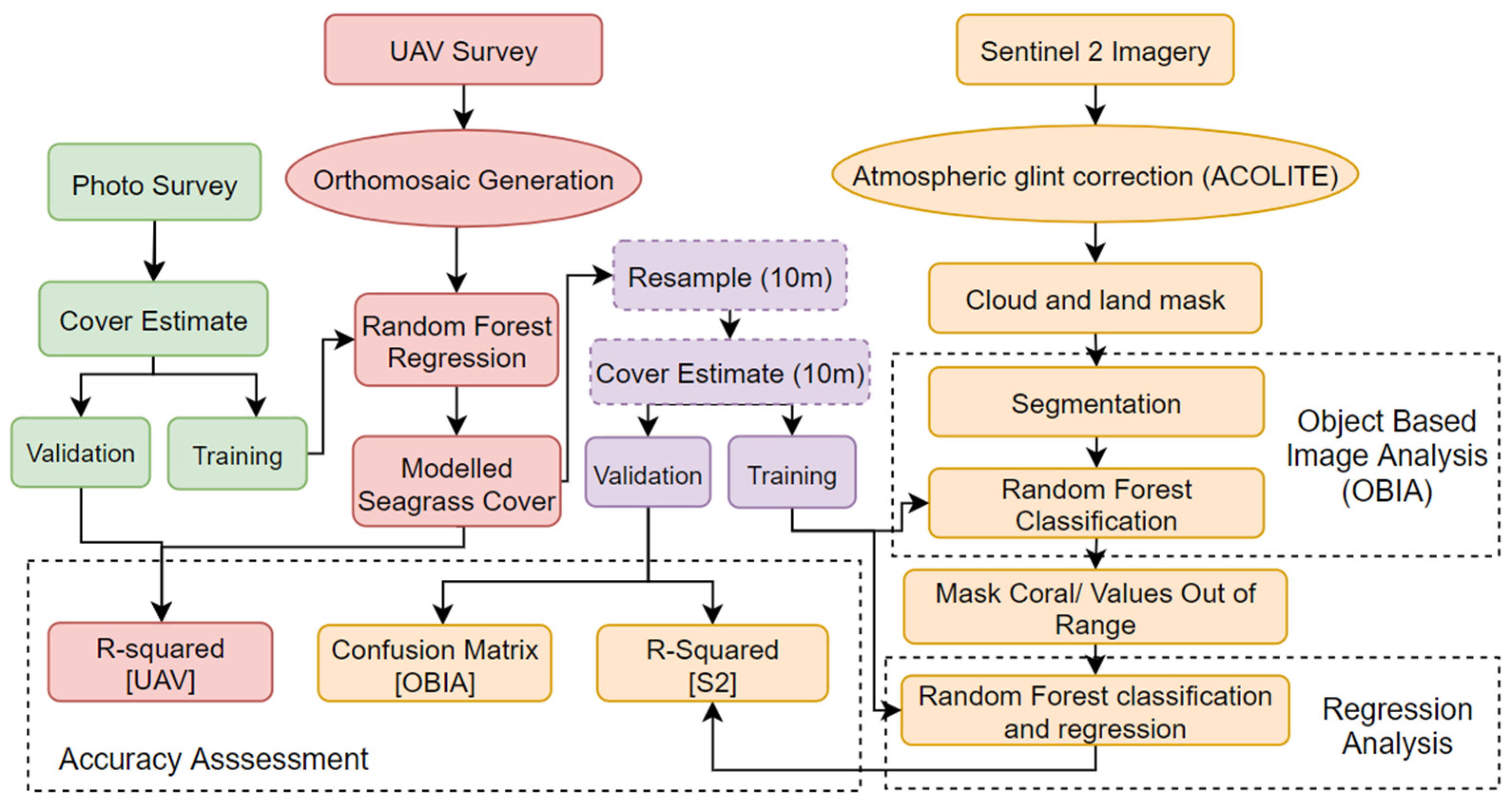
2. Materials and Methods

2.1. Study Site

This survey was carried out at Turneffe Atoll (60 km long, 16 km wide) (Figure 1), one of three atolls in Belize surrounded by a coral reef, consisting of a group of cays (islands). The three atolls and 1065 islands comprise 3% of Belize’s land area [33] and are recognised by the Government of Belize as ecologically important, receiving status as a marine reserve in 2012. Seagrass is widespread across the atoll and consists of various species between the fringing reef, the shore and the central lagoon. UAV surveys were conducted between 23 and 26 January 2019 at four locations selected for their distinct environmental conditions and seagrass communities. Sites A to C were located on the Atlantic side of the atoll and supported populations of Syringodium filiforme Kützing (manatee grass) (Site A) and Thalassia testudinum Koenig (turtle grass) (Sites B/C). Site D was located on the western coastline, sheltered from the Atlantic waves and populated by Halodule wrightii Asherson (shoal grass).

2.2. UAV Data Collection, Processing and Classification

UAV surveys were conducted using a Phantom 4 drone with an onboard GPS for georeferencing and a 20-megapixel camera attached to a 3-axis gimbal on its base. Collection, pre-processing and classification of the UAV data are reported in Price et al [34]). In brief, at each location, low-altitude UAV surveys were taken between 14:30 and 17:30 (local time) to ensure maximum illumination while minimising sun glint. The drone was flown in a boustrophedonic (lawn mower) pattern with waypoints pre-programmed in pix4DCapture, a survey planning software for drone mapping. Flights commenced at 80–100 m altitude, generating <5 cm pixel size images at each site. Images were merged in Agisoft PhotoScan using georeferencing data and ‘Generic’ and ‘Reference’ preselection settings with a key and tie limit of 40,000 and 4000 points per image, respectively [35]. Ground-truthing sites were randomly distributed over the survey areas, and 50 cm2 quadrats were photographed with a submersible GoPro camera. A total of 33 quadrats were deployed at the four sites, ranging between 0 and 100%, and 38 additional theoretical quadrats were drawn from manual interpretation from the imagery in areas of high confidence (i.e., 100% sand or seagrass). A seagrass cover statistic, defined here as the percentage of seagrass visible from birds-eye view [36], was generated from the mean of seven independent subject estimations in the quadrat photo and then used to train and validate a classification. The in situ data from the four sites were combined to perform a single random forest regression as multispectral satellite data have previously been deemed incapable of distinguishing seagrass species [22]. Non-seagrass areas were clipped from the UAV images so the satellite pixels could be modelled for a percentage cover value.
A random forest regression was employed using geoprocessing tools in ArcGIS Pro 2.8 given its utility for modelling continuous variables and track record of predicting terrestrial canopy cover and benthic habitats [37,38]. Random forest is a supervised machine learning technique that uses many decision trees for predictions, and an average of numerous trees are used to prevent overfitting in the model [39]. The accuracy of the classification was determined using an R2 and variance explained percentage.

2.3. Satellite Data Collection and Processing
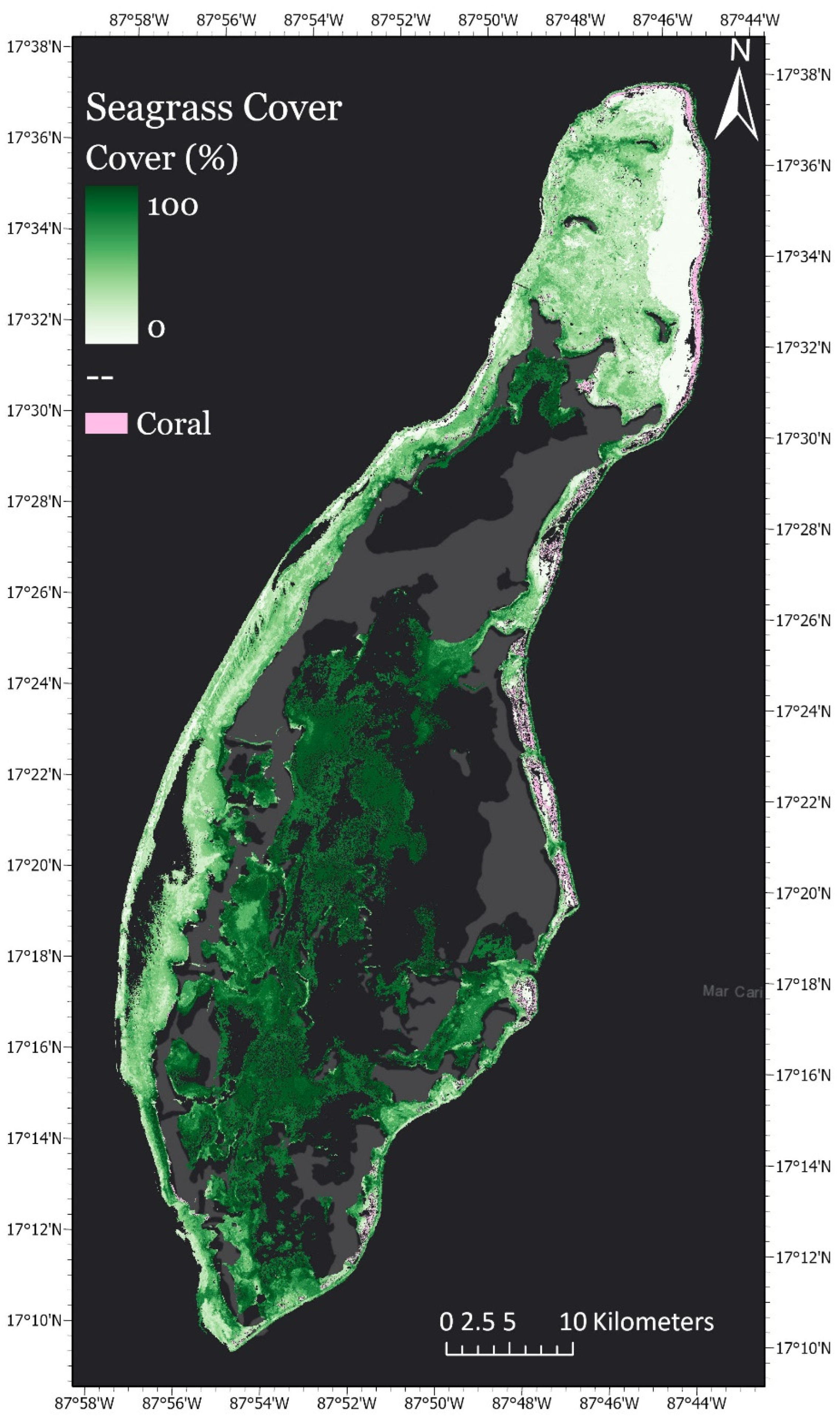
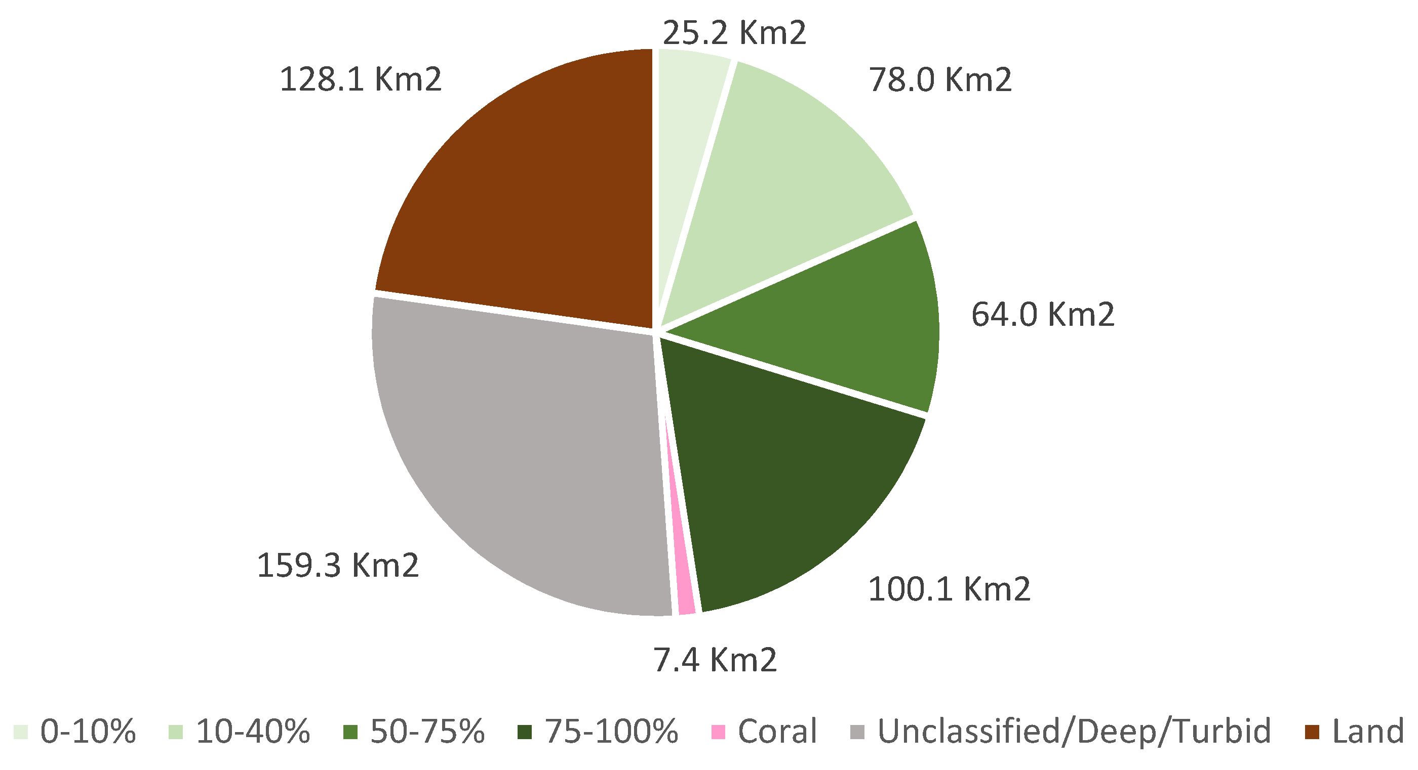
Two Sentinel-2 images of Turneffe Atoll collected on 13 December 2018 were selected for their minimal cloud cover. The time difference between the collection of the satellite and UAV images likely had minimal impact on the reflectance due to the small tidal range in Belize (0.6 m; Table S1). A large tidal difference would alter the value of seagrass cover from a difference in depth and subsequent light attenuation. There was also an absence of storm events in the intervening period between the UAV and satellite datasets. Sentinel-2 L1C data were corrected for atmospheric conditions using the open-source tool ACOLITE [40] as it performs well above coastal waters [41]. Sea surface glint was also corrected in ACOLITE using the short-wave infrared bands at a value of 0.07, which is effective for deeper waters [42,43] (the default set to 0.05). Suspended particulate matter (SPM) concentration was determined using the algorithm of Nechad et al. (2016) for Sentinel-2. In-water SPM directly relates to underwater light attenuation, a critical factor in seagrass distribution, which relies on sunlight for development. Land and wave white cap masks were built using a threshold value of 0.03 in the near-infrared band. Two depth-invariant bands were developed using the red, green and blue bands following a log-linear transformed linear model [44,45] to account for depth. A total of 1536 sandy points were drawn to represent invariant zones at different depths using the Sentinel imagery and ArcPro World Imagery layer, sourced from Maxar data at 0.5 m resolution (from 6 March 2017) [46].
Object-based image analysis (OBIA) was carried out in ArcGIS Pro 2.8 to classify and remove coral areas, and a pixel-based regression was used to retrieve a continuous value of seagrass. It was assumed, based on field observations, that there were no other benthic habitats across the study area, and no discrimination between seagrass species is given. A training sample was extracted by resampling the UAV classifications to the Sentinel-2 grid, averaging the percentage cover statistic to each 10-meter pixel and then converting the raster to a point dataset. The points were thinned to reduce spatial autocorrelation and create an evenly distributed training dataset. A stratified random sample was used to extract an even number of points within 20% cover intervals. For the OBIA, manually labelled points were added in areas of sand and coral using the same Sentinel imagery and ArcPro World Imagery layer used to create the sandy regions for invariant zones as these areas were easily discriminated. For the regression, 25 randomly sampled points from sandy regions were added to the UAV-based estimations to extend the minimum training data value from 4.4 to 0%. Global Moran’s I [47], an index of spatial autocorrelation, was used to determine the level of clustering within the training data. Moran’s I ranges from −1 to 1, where positive values indicate clustering and negative values indicate spatially dispersed data.
Pixels were grouped based on spectral and spatial characteristics using the segment mean shift tool in ArcPro. The parameters ‘minimum segment size in pixels’, ‘spectral detail’ and ‘spatial detail’ had set values of 1, 20 and 17, respectively, and applied to the blue, green, invariant and SPM bands. The red band was removed due to the fast absorption in the water column that would positively skew to denser seagrass covers. The blue, green and SPM bands were logged to remove bias and improve model performance as they demonstrated a positively skewed distribution within the training data. The segmentation quality of the captured benthic environments was optimised by trial-and-error and a random forest classification was used on the segmented image. Seagrass cover was split into the following classes to optimise the accuracy of the coral and deep-water areas: 1–10%, 10–40%, 40–70% and 70–100%. The results were evaluated by calculating overall user and producer accuracy for the OBIA classification. Producer accuracy shows the probability that a given class was classified correctly, and user accuracy is the probability that a value predicted to be in a specific class is in that class [48].
Any variables with values outside the range of the training data were masked along with coral areas found in the OBIA classification. A pixel-based random forest regression was then performed in ArcPro using the blue, green, SPM and depth-invariant bands in the non-segmented Sentinel-2 image. A second regression run was also performed with positional information by including the x and y positions as independent variables into the model, as reports from Mascaro [49] show that modelling can improve whilst reducing spatial autocorrelation. Due to the inherent randomness of the random forest model, the model stability of the best performing regression was assessed by repeating the validation process 100 times to visualise the variation of the R2 and variable importance. The importance of each variable, or band, was evaluated using the Gini coefficient [50], which indicates the stability and drivers of the model. The training and validation datasets were randomly split into 67% for training and 33% for validation, with each iteration extracting a different sample. A summary of the methods is illustrated in Figure 2.

3. Results

3.1. UAV Classifications

The random forest classification for the UAV sites, between the green band and seagrass cover, had an adjusted R2 of 0.91 (p-value < 0.05), and 94.2% of the variation was explained by the model. High seagrass cover was more dominant in Sites A and D, which were less patchy than Sites B and C (Figure 3). Once percentage cover within the footprint of the Sentinel-2 pixels was summarised and a stratified sample had thinned the data, a total of 6682 points, with an average seagrass cover of 50%, were available for training and validation. Based on these results, the seagrass cover values ranged from 4.4 to 96.0%. The Moran’s I score demonstrated that both datasets were clustered, with the thinned data scoring 0.186. After thinning, the z-score reduced by 61%, indicating that the clustering was less intense.

3.2. Satellite Pre-Processing

The satellite pre-processing resulted in a land-masked, glint- and cloud-corrected image and two depth-invariant layers (Figure 4). The blue/green depth-invariant band illustrates a sharp rise in pixel number, as shown by the darker pixels, in less reflective waters at the centre of the atoll. The increased water depth and greater attenuation of light mean that large differences between the blue and green bands are reflected in the data. In the atoll centre, which consists of an 8-meter deep lagoon [51], the reflectance in the green band is far higher than that in the blue, suggesting that seagrass is present. Reflectance in the green band is absorbed more quickly than in the blue over a sandy benthic type assuming minimal dissolved matter [52]. Seagrass was observed in the lagoon, in agreement with local testimony, but it is difficult to estimate the percentage cover without validation data and low reflectance, thus preventing a visual interpretation of seagrass. When removing values outside the range of training data, highly turbid and deep-water areas, such as the centre of the atoll, were masked.

3.3. Object-Based Classification

The overall accuracy of the OBIA map was 48% (Table 1). Despite the low producer accuracy of coral, 91% of the areas mapped as coral were correctly identified, as signified by the user accuracy. Discrimination between seagrass and coral improved when modelling the seagrass from a presence/absence to a classified cover schema, which prompted its use to identify coral areas. However, as demonstrated by the lower producer accuracy of coral areas, there was confusion with the 10–40% seagrass cover and sandy areas (Table S2). This confusion overpredicted the area of seagrass and sand, where coral is usually present. Based on the relatively balanced user and producer accuracies of the seagrass cover classes above 10%, they were neither over- nor underestimated.

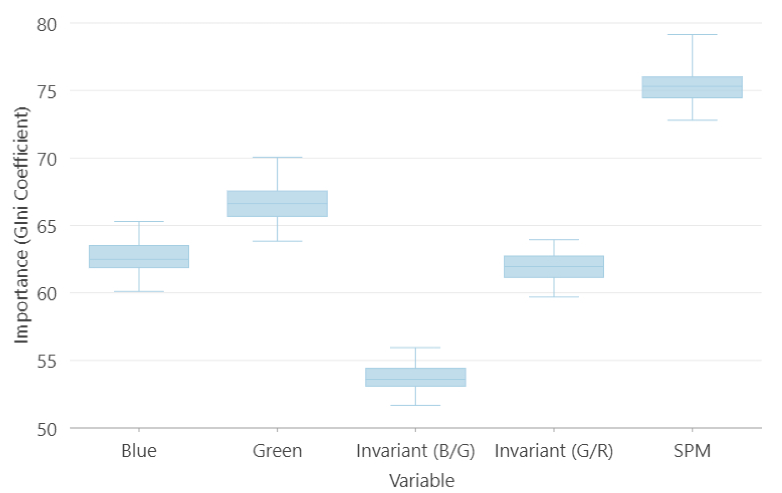
3.4. Pixel-Based Regression

Following the extraction of coral, and areas out of the range of the training data, the regression model produced a seagrass cover map of Turneffe Atoll (Figure 5) with a mean adjusted R2 of 0.73 (p-value < 0.05), explaining 56% of the variation using the blue, green, invariant and SPM bands.
The inner-eastern side of the atoll and a large pocket of the outer-western edge were masked as they were out of the range of the training data (usually deeper or turbid waters). According to the map, Turneffe Atoll consists of 43% seagrass (above 10% cover), 30% land (including mangroves), 4% sand, very sparse seagrass (1–10%) and 1% coral, with 36% of the area out of the range of the training data (Figure 6).
When performing a regression with positional information, the R2 reduced slightly to 0.71 (p-value < 0.05) and 67.5% of the variation was explained. Across the 100 validation runs, the random forest model remained consistent, as shown by the distribution of R2 values (Figure S2), where half are between 0.72 and 0.74. Variation in the Gini coefficient shows that the SPM band was responsible for the split between trees in the random forest model and therefore explains most of the variance in seagrass cover (Figure 7). This importance is followed by the blue, green and green/red invariant bands, each of which explained a similar level of importance. The blue/green invariant band provided the least importance.

4. Discussion

We successfully employed several validated UAV datasets to build a dataset to predict continuous seagrass cover using satellite imagery. To our knowledge, this is the first time this approach has been used, and we propose that its various advantages make it highly suitable to enable the monitoring of technically challenging, submerged vegetated environments. Specifically, we successfully estimated the seagrass percentage cover for over 267 km2 of the shallow waters of Turneffe Atoll, Belize, the largest atoll in the northern hemisphere.
Our method has the potential to ease the logistical and financial burdens associated with the repeated surveys required to establish the presence of stressors or assessment of the effectiveness of management interventions. This is primarily because it reduces the need to collect profuse in situ ground-truthing points, typically conducted via underwater photography of randomly placed quadrats. In addition, our study demonstrates the value of a multistage validation dataset, building upon recent efforts to map seagrass percentage coverage [22].
The UAV classifications of seagrass cover are highly accurate, supporting their use in interpreting cover within the satellite pixels and making available an extensive dataset to train and calibrate satellite imagery. The number of points increased by a factor of 94 between the in situ data collection and thinned UAV points. By incorporating UAV data in this approach, the time required per data point reduced considerably, therefore lowering the cost of data collection. Using this method generated 3320 points from the UAV data post-thinning, whereas 96 were generated using the standard data collection methods of Fauzan [22].
Nevertheless, the advantage of combining UAVs in satellite mapping comes at a cost, as a greater level of spatial autocorrelation will have introduced bias within the model. Ideally, for Turneffe Atoll, several more UAV surveys or a corridor survey could encompass deeper environments and broader coverage to offer a more extensive and evenly distributed sample with a reduced level of spatial autocorrelation. Additionally, any errors within the prediction of seagrass cover in the UAV data, including errors in the estimation of cover within the quadrats, can propagate into the satellite estimates. The potential error propagation emphasises the importance of highly accurate estimates of seagrass cover in UAV imagery to ensure that the satellite data are trained with the least uncertainty compared to point-based techniques. Further research should look into a framework for assessing the transfer of errors between the three datasets. Additionally, studies on the comparison between modelling seagrass cover using UAV-derived data against point-based data collection would be valuable to quantify the benefit of using data from a more representative source.
The high resolution of the UAV data means that their use with in situ data collection offers several advantages: (a) the spatial extent is greater and includes deeper and less accessible waters, (b) a more comprehensive range of seagrass percentage cover values can be collected within the sample and (c) more data become available for training the classifier. These advantages facilitate increased frequency of fine-scale monitoring, which is vital to better understand the impact of changing environmental conditions, providing ecosystem services [15] and informing coastal management and restoration activities [53].
A simple classification schema was chosen to define three unambiguous classes, namely sand, seagrass and coral, to describe the benthic habitats of Turneffe Atoll. These typologies were selected as they capture the dominant sub-tidal habitats present, although a broader, more detailed range could be included in future studies. Macroalgae constitute another crucial component of the ecosystem that is useful to map to a fine scale given that they serve as a blue carbon store and can be used as an indicator of coral health [53,54]. Macroalgae often grow on hard substrates [55] or can be present in sandy areas as turf macroalgae, which can be discriminated against using bathymetry and rugosity [53].
Coral areas were mapped effectively most of the time for the OBIA, as indicated by the user accuracy. With a darker spectral signature than sand, some of the coral areas not identified will have subsequently overpredicted seagrass cover in the regression model. Furthermore, the analysis used expert labelling rather than in situ data; therefore, the distribution of corals should be interpreted with caution. Corals are commonly challenging to distinguish with satellite data due to the high likelihood of the 10-m pixel including other substrates such as sand, algae or detritus, which leads to misclassification [22,53]. Some studies have attempted to use spectral unmixing, a process to decompose a pixel’s spectral signature, to provide more detail on pixels’ composition [53]. Generally, the seagrass cover classes were less accurate when compared to coral, particularly the 1–10% class. However, lower accuracy in the 1–10% was expected given the relatively small training sample compared to the other cover classes, in agreement with accuracy reports from Roelfsema [1] and Kovacs [23]. The accuracy can be partly attributed to its narrower cover window and its similarity to the other cover classes and sandy areas that dominate the pixel.
The seagrass map presents a greater level of detail of seagrass distribution than previous attempts at Turneffe Atoll, the two latest being a three-class seagrass density map in 2014 [56] and a presence/absence map of ecosystems services in 2001 [57], which was later updated in 2004 [58]. The map indicates that high seagrass cover is dominant in areas where we expect low-energy hydrodynamic waters, such as the central lagoon, and along the fringe of mangroves on the western side of the atoll. The eastern side of the lagoon is particularly turbid and difficult to map; hence, it was out of the range of data to model in our map. The southern region of this area was surveyed within the project, with evidence of seagrass (Table S3); however, it was discounted to its poor clarity within the UAV images. Furthermore, previous maps developed in 2014 showed similar results, though it is challenging to quantify change without a high-resolution map or knowledge of how the map was developed. Still, the seagrass cover map here demonstrates that seagrass is a dominant benthic habitat across Turneffe Atoll, in agreement with previous estimations, thus solidifying the area’s importance as a marine reserve. We have created a Google Earth Engine application (https://stcarp.users.earthengine.app/view/turneffe-atoll-seagrass-cover-app (accessed on 16 January 2022)) to provide the first interactive and holistic view of seagrass percentage cover for readers and coastal managers to view, download and query the data to enable effective management strategies. This baseline map can inform subsequent seagrass cover maps to facilitate change analysis for future monitoring efforts.
The model outperformed the results obtained by Fauzan [22], suggesting that the inclusion of two invariant bands with the blue, green and SPM bands gives a more accurate estimation of seagrass cover. The results are more comparable to those carried out in a larger area over northwest Florida [25]. Hyperspectral EO-1 Hyperion and Landsat 5 data, with a 30-meter spatial resolution, recorded an R2 of 0.78 and 0.59, respectively. The high R2 value in the Hyperion data is described as a likely result of the high number of bands used, but with Hyperion discontinued in 2017 and limited availability worldwide, it remains an impractical dataset to use within long-term coastal zone management plans. Contrary to previous suggestions [49], we did not find that positional information improved the model.
One of the most notable findings from this study is the importance of the SPM band in the modelling of seagrass cover. Over the validation runs, the SPM band was consistently the most important variable when determining seagrass cover. From our understanding, this variable has, until now, been neglected within seagrass mapping studies using satellite data, despite evidence that suspended sediment may be the second most determining factor for seagrass growth after temperature [59]. Optimal conditions for seagrass growth require low suspended sediment concentrations to allow greater light penetration into the water column [60]. Additionally, the SPM band is a quick and straightforward addition when using the ACOLITE atmospheric processor as it is included as one of the optional outputs in the processing chain. Whilst sea surface temperature could be accounted for using AVHRR (1 km) or MODIS (250 m) [61], the coarse resolution restricts their use within complex coastal regions.
When compared to the SPM band, the invariant bands are less influential within the model. It is expected that the absence of data from deeper areas means that it is difficult to assess the impact of including the blue and green bands given that they are relatively more absorbed as depth increases. All the UAV survey sites were located in near-shore shallower waters; thus, it is unsurprising that the effectiveness of the invariant band is not apparent. Surveys in deeper waters would confirm whether the predicted high seagrass cover located in the centre of the atoll is accurate. Acquiring deep-water surveys would help to overcome the challenge of distinguishing seagrass cover in deeper waters and define the maximum depth at which the satellite can retrieve seagrass cover information in this area. As with estimating seagrass cover, UAV-derived bathymetry from empirical algorithms such as those in Stumpf et al. (2003) and Lyzenga et al. (2006) or Structure from Motion techniques [62,63] could be used to estimate bathymetry across the atoll using satellites [25]. Incorporating elevation and its derivatives (slope/aspect/rugosity) into seagrass cover models may have improved the predicting power. The addition of another invariant band, produced by downscaling the coastal aerosol band, could also give further improvements, as it has been demonstrated to provide additional information in deeper water [64].
Confusion between the seagrass classes in the OBIA did not appear to affect the pixel-based regression accuracy notably. Nevertheless, the areal change between the two classifications in the 0–10% class was large compared to the areal statistics (Figure S3). Although the minimum object within the segmentation process was set to the pixel size of the satellite, as with previous studies [1], areas of medium to low seagrass cover areas are captured within pixels, which include more sand. Subsequently, earlier estimates in the literature may be underestimating seagrass cover. Whilst object-based methods may be effective for well-defined or featured areas such as urban areas or tree canopies [65], the technique is less effective at grouping continuous variables. The deficient user and producer accuracies indicate that areal statistics are likely inaccurate within the OBIA methods, while the regression gives more precise information than simpler ranked thematic classes [2,20]. Continuous variables can be challenging to estimate, but a higher resolution can help to distinguish patterns between seabed habitats that would otherwise be missed. Further studies on the comparison between modelling seagrass cover using UAV-derived data against point-based data collection would be valuable to quantify the benefit of using data from a more representative source.
Detailed and accurate seagrass cover maps are essential to implement more sophisticated inventories of carbon in wetland regions and reach IPCC tier 3 reports of habitat-specific estimates for blue carbon [66]. Unfortunately, seagrass maps across Belize, like many locations, have been limited to presence/absence maps, which fail to provide enough detail describing how seagrass is deteriorating or recovering. We expect that modelling seagrass cover using this approach will better inform seagrass carbon stocks; specifically, biomass estimates can only be derived when cover data is available [67].

5. Conclusions

Here, we present an alternative means to map seagrass using moderate-resolution satellites and UAVs to expand the training data size considerably compared to traditional in situ methods. The approach overcomes the limitations of previous seagrass mapping exercises, which assume uniform seagrass cover within a satellite pixel and include small training samples. Irrespective of which satellite is used to monitor seagrass, a series of highly accurate UAV classifications offer the ability to increase the data available to train and validate satellites and improve estimates of cover within a pixel rather than generalising point-based field surveys. Future efforts to map seagrass cover should incorporate estimates of suspended particulate matter in the water column as it explains more variation in seagrass cover than a single optical band. Further research into the inclusion of UAV- and satellite-derived bathymetry, as well as a more widespread and extensive set of UAV surveys, is needed to explore how seagrass cover is successfully estimated in deeper waters. Adopting these inclusions should improve the cover estimates of seagrass to the water depth that optical imagery can achieve. This protocol provides a mechanism to monitor seagrass in more detail, which would otherwise be missed using thematic groupings or within the segmentation process in object-based analysis. Over time, repeated maps can help generate more precise statistics on gains and losses of seagrass to identify areas that are deteriorating or recovering in response to coastal processes to help well-informed and effective conservation management.

Supplementary Materials

The following are available online at https://www.mdpi.com/article/10.3390/rs14030477/s1, Table S1: Accuracy of OBIA classification; Table S2: Class confusion matrix OBIA; Figure S1: UAV and Sentinel-2 composites and classifications for each study area; Figure S2: Distribution of R2 values across 100 validation runs; Figure S3: Distribution of seagrass cover classes for the first-stage (OBIA) and second-stage (pixel) classifications. Sand is included as 0–10% cover class.

Author Contributions

Conceptualisation, S.C.; data curation, S.C. and S.L.F.; formal analysis, S.C.; funding acquisition, C.E.; investigation, S.C., D.M.P., S.L.F., V.A., E.C., A.L., H.B. and C.B.; methodology, S.C., V.B. and J.S.; project administration, S.L.F., V.A., A.Y. and C.E.; validation, S.C.; visualisation, S.C.; writing—original draft, S.C., S.L.F. and C.E.; writing—review and editing, S.C., S.L.F., D.M.P., J.S., A.L., H.B., C.B., A.F., R.S. and C.E. All authors have read and agreed to the published version of the manuscript.

Funding

The Government of the United Kingdom supported this work through the Commonwealth Marine Economies Programme, which aims to enable safe and sustainable marine economies across Commonwealth Small Island Developing States. C.E. was supported by a Natural Environment Research Council (NERC) ‘Omics’ Independent Research Fellowship NE/M018806/1. S.L.F. and D.P. received additional support from the Natural Environmental Research Council (grant no. NE/L002531/1 and NE/N012070/1, respectively).

Data Availability Statement

View, query and download the data by the following link—https://stcarp.users.earthengine.app/view/turneffe-atoll-seagrass-cover-app, accessed on 16 January 2022.

Acknowledgments

We would like to thank our Belizean partners in the Turneffe Atoll Sustainability Association (TASA) and the Coastal Zone Management Authority and Institute (CZMAI), including Ellis Requena, Maurice Westby, Jayron Young and Estela Requena, for their logistical support and for hosting the field team.

Conflicts of Interest

The authors declare no conflict of interest.

References

  1. Roelfsema, C.M.; Lyons, M.; Kovacs, E.M.; Maxwell, P.; Saunders, M.I.; Samper-Villarreal, J.; Phinn, S.R. Multi-temporal mapping of seagrass cover, species and biomass: A semi-automated object based image analysis approach. Remote Sens. Environ. 2014, 150, 172–187. [Google Scholar] [CrossRef]
  2. Phinn, S.; Roelfsema, C.; Dekker, A.; Brando, V.; Anstee, J. Mapping seagrass species, cover and biomass in shallow waters: An assessment of satellite multi-spectral and airborne hyper-spectral imaging systems in Moreton Bay (Australia). Remote Sens. Environ. 2008, 112, 3413–3425. [Google Scholar] [CrossRef]
  3. McKenzie, L.J.; Nordlund, L.M.; Jones, B.L.; Cullen-Unsworth, L.C.; Roelfsema, C.; Unsworth, R.K. The global distribution of seagrass meadows. Environ. Res. Lett. 2020, 15, 074041. [Google Scholar] [CrossRef]
  4. Perillo, G.; Wolanski, E.; Cahoon, D.R.; Hopkinson, C.S. Coastal wetlands: An integrated ecosystem approach; Elsevier: Amsterdam, The Netherlands, 2018. [Google Scholar]
  5. Barbier, E.B.; Hacker, S.D.; Kennedy, C.; Koch, E.W.; Stier, A.C.; Silliman, B.R. The value of estuarine and coastal ecosystem services. Ecol. Monogr. 2011, 81, 169–193. [Google Scholar] [CrossRef]
  6. Lilley, R.J.; Unsworth, R.K. Atlantic Cod (Gadus morhua) benefits from the availability of seagrass (Zostera marina) nursery habitat. Glob. Ecol. Conserv. 2014, 2, 367–377. [Google Scholar] [CrossRef] [Green Version]
  7. Unsworth, R.K.; Nordlund, L.M.; Cullen-Unsworth, L.C. Seagrass meadows support global fisheries production. Conserv. Lett. 2019, 12, e12566. [Google Scholar] [CrossRef]
  8. Pham, T.D.; Xia, J.; Ha, N.T.; Bui, D.T.; Le, N.N.; Tekeuchi, W. A review of remote sensing approaches for monitoring blue carbon ecosystems: Mangroves, seagrassesand salt marshes during 2010–2018. Sensors 2019, 19, 1933. [Google Scholar] [CrossRef] [PubMed] [Green Version]
  9. Newell, R.I.; Koch, E.W. Modeling seagrass density and distribution in response to changes in turbidity stemming from bivalve filtration and seagrass sediment stabilization. Estuaries 2004, 27, 793–806. [Google Scholar] [CrossRef]
  10. Ceccherelli, G.; Oliva, S.; Pinna, S.; Piazzi, L.; Procaccini, G.; Marin-Guirao, L.; Dattolo, E.; Gallia, R.; La Manna, G.; Gennaro, P.; et al. Seagrass collapse due to synergistic stressors is not anticipated by phenological changes. Oecologia 2018, 186, 1137–1152. [Google Scholar] [CrossRef]
  11. Short, F.T.; Wyllie-Echeverria, S. Natural and human-induced disturbance of seagrasses. Environ. Conserv. 1996, 23, 17–27. [Google Scholar] [CrossRef]
  12. Saunders, M.I.; Leon, J.; Phinn, S.R.; Callaghan, D.P.; O’Brien, K.R.; Roelfsema, C.M.; Lovelock, C.E.; Lyons, M.B.; Mumby, P.J. Coastal retreat and improved water quality mitigate losses of seagrass from sea level rise. Glob. Chang. Biol. 2013, 19, 2569–2583. [Google Scholar] [CrossRef]
  13. Fraser, M.W.; Kendrick, G.A. Belowground stressors and long-term seagrass declines in a historically degraded seagrass ecosystem after improved water quality. Sci. Rep. 2017, 7, 14469. [Google Scholar]
  14. A’an, J.W.; Rahmawati, S.; Irawan, A.; Hadiyanto, H.; Prayudha, B.; Hafizt, M.; Afdal, A.; Adi, N.S.; Rustam, A.; Hernawan, U.E. Assessing Carbon Stock and Sequestration of the Tropical Seagrass Meadows in Indonesia. Ocean Sci. J. 2020, 55, 85–97. [Google Scholar]
  15. Farina, S.; Guala, I.; Oliva, S.; Piazzi, L.; Pires da Silva, R.; Ceccherelli, G. The seagrass effect turned upside down changes the prospective of sea urchin survival and landscape implications. PLoS ONE 2016, 11, e0164294. [Google Scholar] [CrossRef] [PubMed] [Green Version]
  16. Björk, M.; Short, F.; Mcleod, E.; Beer, S. Managing Seagrasses for Resilience to Climate Change; IUCN: Gland, Switzerland, 2008. [Google Scholar]
  17. Hossain, M.; Bujang, J.; Zakaria, M.; Hashim, M. The application of remote sensing to seagrass ecosystems: An overview and future research prospects. Int. J. Remote Sens. 2015, 36, 61–114. [Google Scholar] [CrossRef]
  18. Hedley, J.D.; Roelfsema, C.M.; Chollett, I.; Harborne, A.R.; Heron, S.F.; Weeks, S.; Skirving, W.J.; Strong, A.E.; Eakin, C.M.; Christensen, T.R. Remote sensing of coral reefs for monitoring and management: A review. Remote Sens. 2016, 8, 118. [Google Scholar] [CrossRef] [Green Version]
  19. Pasqualini, V.; Pergent-Martini, C.; Pergent, G.; Agreil, M.; Skoufas, G.; Sourbes, L.; Tsirika, A. Use of SPOT 5 for mapping seagrasses: An application to Posidonia oceanica. Remote Sens. Environ. 2005, 94, 39–45. [Google Scholar] [CrossRef]
  20. Topouzelis, K.; Spondylidis, S.C.; Papakonstantinou, A.; Soulakellis, N. The use of Sentinel-2 imagery for seagrass mapping: Kalloni Gulf (Lesvos Island, Greece) case study. In Proceedings of the Fourth International Conference on Remote Sensing and Geoinformation of the Environment (RSCy2016), Paphos, Cyprus, 4 April 2016; p. 96881F. [Google Scholar]
  21. Traganos, D.; Reinartz, P. Mapping Mediterranean seagrasses with Sentinel-2 imagery. Mar. Pollut. Bull. 2018, 134, 197–209. [Google Scholar] [CrossRef] [Green Version]
  22. Fauzan, M.A.; Kumara, I.S.; Yogyantoro, R.; Suwardana, S.; Fadhilah, N.; Nurmalasari, I.; Apriyani, S.; Wicaksono, P. Assessing the capability of Sentinel-2A data for mapping seagrass percent cover in Jerowaru, East Lombok. Indones. J. Geogr. 2017, 49, 195–203. [Google Scholar] [CrossRef] [Green Version]
  23. Kovacs, E.; Roelfsema, C.; Lyons, M.; Zhao, S.; Phinn, S. Seagrass habitat mapping: How do Landsat 8 OLI, Sentinel-2, ZY-3A, and Worldview-3 perform? Remote Sens. Lett. 2018, 9, 686–695. [Google Scholar] [CrossRef]
  24. Zoffoli, M.L.; Gernez, P.; Rosa, P.; Le Bris, A.; Brando, V.E.; Barillé, A.-L.; Harin, N.; Peters, S.; Poser, K.; Spaias, L. Sentinel-2 remote sensing of Zostera noltei-dominated intertidal seagrass meadows. Remote Sens. Environ. 2020, 251, 112020. [Google Scholar] [CrossRef]
  25. Pu, R.; Bell, S.; Meyer, C.; Baggett, L.; Zhao, Y. Mapping and assessing seagrass along the western coast of Florida using Landsat TM and EO-1 ALI/Hyperion imagery. Estuar. Coast. Shelf Sci. 2012, 115, 234–245. [Google Scholar] [CrossRef]
  26. Barrell, J.P. Quantification and Spatial Analysis of Seagrass Landscape Structure through the Application of Aerial and Acoustic Remote Sensing. Ph.D. Thesis, Dalhousie University, Halifax, NS, USA, 2016. [Google Scholar]
  27. Hamylton, S.M. Mapping coral reef environments: A review of historical methods, recent advances and future opportunities. Prog. Phys. Geogr. 2017, 41, 803–833. [Google Scholar] [CrossRef]
  28. Duffy, J.P.; Pratt, L.; Anderson, K.; Land, P.E.; Shutler, J.D. Spatial assessment of intertidal seagrass meadows using optical imaging systems and a lightweight drone. Estuar. Coast. Shelf Sci. 2018, 200, 169–180. [Google Scholar] [CrossRef]
  29. Rattanachot, E.; Stankovic, M.; Aongsara, S.; Prathep, A. Ten years of conservation efforts enhance seagrass cover and carbon storage in Thailand. Bot. Mar. 2018, 61, 441–451. [Google Scholar] [CrossRef]
  30. Ventura, D.; Bonifazi, A.; Gravina, M.F.; Belluscio, A.; Ardizzone, G. Mapping and classification of ecologically sensitive marine habitats using unmanned aerial vehicle (UAV) imagery and object-based image analysis (OBIA). Remote Sens. 2018, 10, 1331. [Google Scholar] [CrossRef] [Green Version]
  31. Nahirnick, N.K.; Reshitnyk, L.; Campbell, M.; Hessing-Lewis, M.; Costa, M.; Yakimishyn, J.; Lee, L. Mapping with confidence; delineating seagrass habitats using Unoccupied Aerial Systems (UAS). Remote Sens. Ecol. Conserv. 2019, 5, 121–135. [Google Scholar] [CrossRef]
  32. Young, C.A. Belize’s ecosystems: Threats and challenges to conservation in Belize. Trop. Conserv. Sci. 2008, 1, 18–33. [Google Scholar] [CrossRef] [Green Version]
  33. Murray, M.R.; Zisman, S.; Furley, P.A.; Munro, D.M.; Gibson, J.; Ratter, J.; Bridgewater, S.; Minty, C.D.; Place, C. The mangroves of Belize: Part 1. distribution, composition and classification. For. Ecol. Manag. 2003, 174, 265–279. [Google Scholar] [CrossRef]
  34. Price, D.; Felgate, S.; Huvenne, V.; Strong, J.; Carpenter, S.; Barry, C.; Lichtschlag, A.; Sanders, R.; Carrias, A.; Young, A.; et al. Quantifying the Intra-Habitat Variation of Seagrass Beds with Unoccupied Aerial Vehicles (UAVs). Remote Sens. 2022, 14, 480. [Google Scholar] [CrossRef]
  35. Pfeifer, N.; Glira, P.; Briese, C. Direct georeferencing with on board navigation components of light weight UAV platforms. Int. Arch. Photogramm. Remote Sens. Spat. Inf. Sci. 2012, 39, 487–492. [Google Scholar] [CrossRef] [Green Version]
  36. Lyons, M.; Phinn, S.; Roelfsema, C. Integrating Quickbird multi-spectral satellite and field data: Mapping bathymetry, seagrass cover, seagrass species and change in Moreton Bay, Australia in 2004 and 2007. Remote Sens. 2011, 3, 42–64. [Google Scholar] [CrossRef] [Green Version]
  37. Coulston, J.W.; Moisen, G.G.; Wilson, B.T.; Finco, M.V.; Cohen, W.B.; Brewer, C.K. Modeling percent tree canopy cover: A pilot study. Photogramm. Eng. Remote Sens. 2012, 78, 715–727. [Google Scholar] [CrossRef] [Green Version]
  38. Janowski, L.; Wroblewski, R.; Dworniczak, J.; Kolakowski, M.; Rogowska, K.; Wojcik, M.; Gajewski, J. Offshore benthic habitat mapping based on object-based image analysis and geomorphometric approach. A case study from the Slupsk Bank, Southern Baltic Sea. Sci. Total Environ. 2021, 801, 149712. [Google Scholar] [CrossRef] [PubMed]
  39. Breiman, L. Random forests. Mach. Learn. 2001, 45, 5–32. [Google Scholar] [CrossRef] [Green Version]
  40. Vanhellemont, Q.; Ruddick, K. Acolite for Sentinel-2: Aquatic applications of MSI imagery. In Proceedings of the 2016 ESA Living Planet Symposium, Prague, Czech Republic, 9–13 May 2016; pp. 9–13. [Google Scholar]
  41. Ilori, C.O.; Pahlevan, N.; Knudby, A. Analyzing performances of different atmospheric correction techniques for Landsat 8: Application for coastal remote sensing. Remote Sens. 2019, 11, 469. [Google Scholar] [CrossRef] [Green Version]
  42. Harmel, T.; Chami, M.; Tormos, T.; Reynaud, N.; Danis, P.-A. Sunglint correction of the Multi-Spectral Instrument (MSI)-SENTINEL-2 imagery over inland and sea waters from SWIR bands. Remote Sens. Environ. 2018, 204, 308–321. [Google Scholar] [CrossRef]
  43. Keay, R. Atmospheric and Glint Correction of Sentinel-2 Imagery for Marine and Coastal Machine Learning. Available online: https://medium.com/uk-hydrographic-office/atmospheric-and-glint-correction-of-sentinel-2-imagery-for-marine-and-coastal-machine-learning-ec0ea8734e23 (accessed on 21 January 2021).
  44. Lyzenga, D.R. Passive remote sensing techniques for mapping water depth and bottom features. Appl. Opt. 1978, 17, 379–383. [Google Scholar] [CrossRef] [PubMed]
  45. Lyzenga, D.R. Remote sensing of bottom reflectance and water attenuation parameters in shallow water using aircraft and Landsat data. Int. J. Remote Sens. 1981, 2, 71–82. [Google Scholar] [CrossRef]
  46. World Imagery [basemap] 1:132,531 World Imagery Map. 2009. Available online: https://www.arcgis.com/home/item.html?id=10df2279f9684e4a9f6a7f08febac2a9 (accessed on 21 January 2021).
  47. Getis, A.; Ord, J.K. The Analysis of Spatial Association by Use of Distance Statistics. Geogr. Anal. 1992, 24, 189–206. [Google Scholar] [CrossRef]
  48. ESRI. Resampling Method (Environment Setting)—Geoprocessing|ArcGIS Desktop. Available online: https://pro.arcgis.com/en/pro-app/tool-reference/environment-settings/resampling-method.htm (accessed on 14 August 2021).
  49. Mascaro, J.; Asner, G.P.; Knapp, D.E.; Kennedy-Bowdoin, T.; Martin, R.E.; Anderson, C.; Higgins, M.; Chadwick, K.D. A tale of two “forests”: Random Forest machine learning aids tropical forest carbon mapping. PLoS ONE 2014, 9, e85993. [Google Scholar] [CrossRef]
  50. Gini, C. Variabilità e Mutabilità; Libreria Eredi Virgilio Veschi: Rome, Italy, 1912. [Google Scholar]
  51. McCloskey, T.A.; Liu, K.-b. Sedimentary history of mangrove cays in Turneffe Islands, Belize: Evidence for sudden environmental reversals. J. Coast. Res. 2013, 29, 971–983. [Google Scholar] [CrossRef]
  52. Mascarenhas, V.; Keck, T. Marine Optics and Ocean Color Remote Sensing. In YOUMARES 8–Oceans Across Boundaries: Learning from Each Other; Springer: Cham, Switzerland, 2018; p. 41. [Google Scholar]
  53. Poursanidis, D.; Traganos, D.; Teixeira, L.; Shapiro, A.; Muaves, L. Cloud-native Seascape Mapping of Mozambique’s Quirimbas National Park with Sentinel-2. Remote Sens. Ecol. Conserv. 2020, 7, 275–291. [Google Scholar] [CrossRef]
  54. Roff, G.; Mumby, P.J. Global disparity in the resilience of coral reefs. Trends Ecol. Evol. 2012, 27, 404–413. [Google Scholar] [CrossRef]
  55. Macreadie, P.I.; Jarvis, J.; Trevathan-Tackett, S.M.; Bellgrove, A. Seagrasses and macroalgae: Importance, vulnerability and impacts. In Climate Change Impacts on Fisheries and Aquaculture: A Global Analysis; Wiley-Blackwell: Hoboken, NJ, USA, 2017; pp. 729–770. [Google Scholar]
  56. O’Hara, T.D.; Rowden, A.A.; Williams, A. Cold-water coral habitats on seamounts: Do they have a specialist fauna? Divers Distrib 2008, 14, 925–934. [Google Scholar] [CrossRef]
  57. Meerman, J.; Sabido, W. Central American Ecosystems Map: Belize. CCAD/World Bank/Programme Belize. 2001. Available online: http://biological-diversity.info/Ecosystems.htm (accessed on 6 December 2021).
  58. Belize Ecosystem Map: 2004 Version. Available online: http://biological-diversity.info/Ecosystems.htm (accessed on 21 June 2021).
  59. Daud, M.; Pin, T.; Handayani, T. The spatial pattern of seagrass distribution and the correlation with salinity, sea surface temperature, and suspended materials in Banten Bay. In Proceedings of the IOP Conference Series: Earth and Environmental Science, Purwokerto, Indonesia, 5–6 August 2019; p. 012013. [Google Scholar]
  60. Choice, Z.D.; Frazer, T.K.; Jacoby, C.A. Light requirements of seagrasses determined from historical records of light attenuation along the Gulf coast of peninsular Florida. Mar. Pollut. Bull. 2014, 81, 94–102. [Google Scholar] [CrossRef] [PubMed]
  61. Phinn, S.R.; Kovacs, E.M.; Roelfsema, C.M.; Canto, R.F.; Collier, C.J.; McKenzie, L. Assessing the potential for satellite image monitoring of seagrass thermal dynamics: For inter-and shallow sub-tidal seagrasses in the inshore Great Barrier Reef World Heritage Area, Australia. Int. J. Digit. Earth 2018, 11, 803–824. [Google Scholar] [CrossRef]
  62. Casella, E.; Collin, A.; Harris, D.; Ferse, S.; Bejarano, S.; Parravicini, V.; Hench, J.L.; Rovere, A. Mapping coral reefs using consumer-grade drones and structure from motion photogrammetry techniques. Coral Reefs 2017, 36, 269–275. [Google Scholar] [CrossRef]
  63. Skarlatos, D.; Agrafiotis, P. A Novel Iterative Water Refraction Correction Algorithm for Use in Structure from Motion Photogrammetric Pipeline. J. Mar. Sci. Eng. 2018, 6, 77. [Google Scholar] [CrossRef] [Green Version]
  64. Poursanidis, D.; Traganos, D.; Reinartz, P.; Chrysoulakis, N. On the use of Sentinel-2 for coastal habitat mapping and satellite-derived bathymetry estimation using downscaled coastal aerosol band. Int. J. Appl. Earth Obs. Geoinf. 2019, 80, 58–70. [Google Scholar] [CrossRef]
  65. Yadav, S.; Rizvi, I.; Kadam, S. Urban tree canopy detection using object-based image analysis for very high resolution satellite images: A literature review. In Proceedings of the 2015 International Conference on Technologies for Sustainable Development (ICTSD), Mumbai, India, 4–6 February 2015; pp. 1–6. [Google Scholar]
  66. Hiraishi, T.; Krug, T.; Tanabe, K.; Srivastava, N.; Baasansuren, J.; Fukuda, M.; Troxler, T. 2013 Supplement to the 2006 IPCC Guidelines for National Greenhouse Gas Inventories: Wetlands; IPCC: Geneva, Switzerland, 2014. [Google Scholar]
  67. Gullström, M.; Lyimo, L.D.; Dahl, M.; Samuelsson, G.S.; Eggertsen, M.; Anderberg, E.; Rasmusson, L.M.; Linderholm, H.W.; Knudby, A.; Bandeira, S. Blue carbon storage in tropical seagrass meadows relates to carbonate stock dynamics, plant–sediment processes, and landscape context: Insights from the western Indian Ocean. Ecosystems 2018, 21, 551–566. [Google Scholar] [CrossRef] [Green Version]
Figure 1. Turneffe Atoll and the four study sites (starred). Base map: Sentinel-2 mosaic.
Remotesensing 14 00477 g001
Figure 2. Hierarchical structure and flow chart representing the approach to seagrass percentage cover mapping by using UAV data to train and validate Sentinel-2 imagery with a two-stage classification process.
Remotesensing 14 00477 g002
Figure 3. UAV surveys and classifications for each study area. These predictions are visualised against the Sentinel-2 data and seagrass cover estimates in Figure S1.
Remotesensing 14 00477 g003
Figure 4. (a) Sentinel-2 processing. Level 1 RGB composite, (b) Level 2 ACOLITE-corrected (cloud/glint) cloud and land masked RGB composite and (c) the blue/green depth invariant band (also cloud and land masked).
Remotesensing 14 00477 g004
Figure 5. Seagrass cover over Turneffe Atoll after masking of land, coral and values outside the training data range (often deep-water or turbid areas); base map credits: Esri, HERE, Garmin, USGS. Visualise and query this data by following the link—https://stcarp.users.earthengine.app/view/turneffe-atoll-seagrass-cover-app (accessed on 16 January 2022).
Remotesensing 14 00477 g005
Figure 6. Composition of benthic habitats in Turneffe Atoll.
Remotesensing 14 00477 g006
Figure 7. Distribution of variable importance across all validation runs. B/G = blue/green, G/R = green/red, SPM = suspended particulate matter.
Remotesensing 14 00477 g007
Table 1. Accuracy of OBIA classification.
CategoryProducer AccuracyUser Accuracy
Seagrass Cover (%)1–100.170.31
10–400.390.32
40–700.340.36
70–1000.630.55
Coral0.750.91
Sand0.110.73
Overall Accuracy0.48
Publisher’s Note: MDPI stays neutral with regard to jurisdictional claims in published maps and institutional affiliations.

