Article

Transformer for Tree Counting in Aerial Images

Department of Electrical Engineering and Computer Science (EECS), University of Missouri, Columbia, MO 65211, USA
*
Author to whom correspondence should be addressed.
Remote Sens. 2022, 14(3), 476; https://doi.org/10.3390/rs14030476
Submission received: 23 November 2021 / Revised: 10 January 2022 / Accepted: 10 January 2022 / Published: 20 January 2022

Abstract

:
The number of trees and their spatial distribution are key information for forest management. In recent years, deep learning-based approaches have been proposed and shown promising results in lowering the expensive labor cost of a forest inventory. In this paper, we propose a new efficient deep learning model called density transformer or DENT for automatic tree counting from aerial images. The architecture of DENT contains a multi-receptive field convolutional neural network to extract visual feature representation from local patches and their wide context, a transformer encoder to transfer contextual information across correlated positions, a density map generator to generate spatial distribution map of trees, and a fast tree counter to estimate the number of trees in each input image. We compare DENT with a variety of state-of-art methods, including one-stage and two-stage, anchor-based and anchor-free deep neural detectors, and different types of fully convolutional regressors for density estimation. The methods are evaluated on a new large dataset we built and an existing cross-site dataset. DENT achieves top accuracy on both datasets, significantly outperforming most of the other methods. We have released our new dataset, called Yosemite Tree Dataset, containing a 10 km2 rectangular study area with around 100k trees annotated, as a benchmark for public access.

1. Introduction

The density and distribution of forest trees are important information for ecologists to understand the ecosystem in certain regions. For example, the environmental effect of deforestation or forest fires may be estimated based on the number of lost trees and their location. In recent decades, forest trees are often counted with the help of aerial imagery. Since manually counting the trees from images is time-consuming, automatic tree counting methods have been developed to lower the time cost. With the breakthrough of deep learning in the recent decade, deep neural networks (DNNs) made unprecedented progress in computer vision tasks such as image classification [1,2,3,4,5] and object detection [6,7,8,9,10,11]. DNNs also become widely popular for object counting. One approach of object counting using DNNs is detection-based, i.e., to localize each individual object of interest first and then get the total number. So far this is the mainstream of the published tree counting methods [12,13,14,15,16,17,18]. Another approach is to regress the density of objects in the image using DNNs and then calculate object counts. This approach has been successful for crowd (people) counting [19,20,21,22,23]. However, the effectiveness of density-based methods for tree counting are not sufficiently explored as they are reported in much fewer published works with limited comparative evaluation [24,25].
In this work, we propose a new method for tree counting called density transformer or DENT, which consists of a multi-receptive field (Multi-RF) convolutional neural network (CNN), a transformer, and two heads: Density Map Generator (DMG) and tree counter. The Multi-RF CNN extracts visual features from images with multiple receptive fields of different sizes simultaneously, perceiving the patterns of both the local patch and the concentric context. The transformer models the pair-wise relations between the visual features and filters the contextual visual information sharing across different positions using an attention mechanism. The two heads, the DMG, and the tree counter, parallelly decode the hidden states of the transformer to generate the tree density map at different granularity levels. If a relatively coarse treemap already meets the demand, the DMG can be detached after training to save the inference time. The whole model of DENT is end-to-end trainable.
Currently, very few benchmark datasets are publicly available for tree counting tasks. Previous works reported their performances tested on either private data or a small subset (<10k trees) of public datasets made for other tasks [16,26]. The lack of a common benchmark makes fair comparison across different methods difficult. Hence, we created a new labeled dataset called Yosemite Tree Dataset, which contains aerial images for a ∼10 km2 rectangular area with ∼100k trees whose coordinates are annotated. It is suitable for evaluating not only the performance of tree counting methods but also the counting error versus the area of interest. We have released this dataset to the public.
To demonstrate the effectiveness of DENT, we compare DENT with many existing state-of-art methods of different types, including fully convolutional networks regressors and detectors. The methods are evaluated on the Yosemite Tree Dataset and the cross-site NeonTreeEvaluation [16] Dataset. On both of them, DENT achieves competitive results with the best existing methods and significantly outperforms most of the other methods.
The main contributions of this work include two parts. The first part is the novel end-to-end approach for tree counting, using an efficient multi-receptive field CNN architecture for visual feature representation, a transformer for modeling the pair-wise interaction between the visual features, and two heads for outputs at different granularity and time costs. The second part is the new Yosemite Tree Dataset as a common benchmark for tree counting.

2. Related Works

2.1. Transformers

Transformers [27] are attention-based deep learning models. They are initially proposed in the area of natural language processing (NLP). The input of a transformer is an embedding sequence. Pair-wise interaction between any two elements of the sequence is formulated by the transformers. The output corresponding to an element is aggregated from all the elements of the sequence with different weights depending on their relationship. In this paper, we adopt a transformer to enhance the CNN features, by selectively transferring contextual information among different elements.
Transformer-based methods have also been proposed for computer vision tasks such as object detection [11], image classification [28] in recent years. These methods are also applied on remote sensing images such as in  [29,30]. However, to the best of our knowledge, this work is the first work applying a transformer as a density regressor to count objects in aerial images.

2.2. Density Estimation

Learning density maps using deep CNNs is a trend of crowd counting. On this trend, the counting task is formulated as a regression program. The CNNs are trained to predict the density distribution over the input image. However, the location of each individual object is not explicitly predicted. When the object is crowded, the representation of the density map is relatively robust. In the existing works, different network architectures are tried. MCNN [19] uses a multi-column network with different filter sizes for objects at different scales. The features from all the columns are fused to predict the crowd density map. SwitchCNN [20] has an additional classifier to predict and switch to the best column for the given image. CSRNet [21] generates a high-resolution density map. It is composed of a front-end CNN for feature extraction and a back-end CNN for map generation. It uses dilated convolution instead of pooling or transposed convolution to reduce the computational complexity. CANNet [23] encodes contextual information at different scales by subtracting the local average from the feature maps.
For tree counting tasks, an AlexNet [1] regressor is applied in [24]. In the work of [25], AlexNet [1], VGGNet [2], and a UNet [31] are evaluated and compared; the UNet achieves the best performance. In this paper, we follow the paradigm of the density estimation problem and formulate tree counting as a regression problem.

2.3. Object Detection

The purpose of object detection is to localize each object of interest in the image. Traditional detectors explicitly use a sliding window of predefined size to scan each position of the image [32,33,34,35,36]. These early works usually extract hand-crafted features such as HOG [34] and SIFT [37]. These features are finally fed to a classifier such as a support vector machine (SVM) or a neural network. Modern detectors make use of the powerful features from deep convolutional neural networks (CNNs) pre-trained on large-scale classification datasets [1]. These detectors adopt different strategies to generate bounding boxes for objects using CNNs. Faster-RCNN [6], RetinaNet [8], and YOLO [9] predefine a set of anchors and formulate the detection into two sub-problems: classification of the subimage in each anchor and regression of the offset between the ground truth box and the anchor. CenterNet [10] treats the center of an object as a keypoint and regresses the width and height. RetinaNet, YOLO, and CenterNet infer the results in one shot. In contrast, Faster-RCNN recomputes the features for classification after the generation of region proposals.
So far, most of the published works of tree counting methods are based on detection. These methods can be categorized into tree groups:
(1) Explicitly using sliding windows. The very early works in [38,39,40,41] synthesize the expected appearance of trees and generate a template based on the prior knowledge. The likelihood of the existence of a tree in a sliding window is estimated by the correlation between the tree template and the image patch in the window. However, the templates oversimplify the diverse appearance of trees in real world. Later works use hand-crafted features plus classifiers. For example, a feature descriptor using circular autocorrelation is designed to detect the shape of palm tree in [42]. The goal in [43] is also to detect palm tree, but the descriptor used is HOG [34]. While [13,44] using CNNs to recognize palm trees in the sliding window to learn features automatically. TS-CNNs [45] has two sliding windows of different sizes, each has an AlexNet classifier. One is to recognize the pattern of trees, the other one is to suppress the false positives according to the spatial distribution of the surrounding objects.
(2) Fully convolutional classifiers are equivalent to sliding window CNN classifiers but with better computational efficiency. U-Net [31] and DenseNet [46] are used to predict the confidence maps of tree in [47,48]. The peaks on the confidence maps are considered as the final prediction.
(3) Modern CNN detectors like Faster RCNN [6], SSD [7], RetinaNet [8], and YOLOv3 [9] have state-of-art localization performance in general object detection tasks. These approaches are also applied for tree detection in [14,15,16,17,18].
Counting trees in aerial images using detectors is straightforward but with some disadvantages, especially when the trees are dense and crowded. Firstly the representation of overlapping trees may be ambiguous for detectors at test time. A typical detector usually outputs an excessive number of initial boxes and applies Non-Maximum Suppression (NMS) to select the best ones. The basic idea of NMS is to pair-wisely check the Intersection over Union (IoU) of every two proposal boxes, and remove the one with a lower detection score when their IoU is higher than a preset threshold (typically 0.45 or 0.50). For tree counting, it is often the case that two correct boxes have high IoU. An example case is shown in Figure 1b. In this case, the NMS procedure will likely remove either the blue box or the yellow box and cause an underestimation of the tree count. Secondly, the threshold for the detection score directly affects the predicted tree count. Deliberately tuning the threshold requires extra effort. Thirdly, bounding boxes are relatively expensive to label. The labelers need to determine the width and the height of the boxes. It is often difficult when the trees are overlapping.

3. A New Density Transformer, DENT

The architecture of the DENT model is illustrated in Figure 2. It contains four main components: a Multi-Receptive Field convolutional network (Multi-RF CNN) to compute a feature map over an input image, a transformer encoder to model the interaction of features extracted from different positions, a Density Map Generator (DMG) to predict the density of the trees and a counter to regress the number of trees in the image.
Starting from a RGB aerial image I R 3 × H 0 × W 0 , the Multi-RF CNN generates a low-resolution feature map f CNN R C × H × W , where C is the number of output channels, and in this paper H = H 0 32 and W = W 0 32 . The feature map is projected using a trainable linear transform to generate f visual R d model × H × W , where d model is the dimension of the hidden states of the transformer encoder. For convenient, it can also be reshaped and represented in a sequence form: f visual = [ f 0 , f 1 , . . . , f L ] where L = H W and f i R d model . Since each f i is corresponding to a certain position p i in the image, we use it to estimate the tree density at p i . We also use a special embedding f cnt R d model to query the number of trees in the image. The transformer encoder selectively transfers the information across f 0 f L and f cnt . The final hidden state of the transformer are decoded by the DMG and the tree counter. Then the DMG generates a density map D R H × W . Meanwhile, the tree counter outputs the number of trees z ^ R . The details of the components are discussed in the following sections.

3.1. Multi-Receptive Field Network

Inspired by the macula of the human retina, we extract feature presentation of each position of the image using multiple receptive fields, based on the intuitive assumptions: A wide receptive field of CNN covers a large area of the image containing rich contextual information. On the other hand, a narrow one focuses on the details in a small region of interest without being distracted by the surrounding objects.
Early works in MCNN [19] and SwitchCNN [20] control the receptive fields by designing multi-column networks with different convolutional kernel sizes. We argue that such a strategy has limitations: Firstly, using these methods it is not easy to implement a small receptive field on much deeper networks because generally the receptive field is enlarged quickly with the depth of the network increased. Modern deep networks usually have large receptive fields. For example, a VGG16 [2] has a receptive field of 212 × 212 while a ResNet50 [3] has a receptive field of 483 × 483 [49]. Secondly, the widely used pretrained off-the-shelf models cannot be reused. Searching for the optimal architecture and pretraining takes extra effort. To avoid these limitations, We use an off-the-shelf network as a backbone and add jump connections to its early layers to implement small receptive fields.
We proposed Multi-Receptive Field convolutional network (Multi-RF CNN) as depicted in Figure 3. Specifically, the network contains a vanilla ResNet18 and two extra paths added on the convolutional Block 2. We refer to the original path of ResNet18 from Block 2 (i.e., Block 3∼5) as Path A. Path B consists of two 1 × 1 convolutional layers. Path C is simply an average pooling layer. The strides of the three paths are all the same as 32 on the original input image. The receptive fields of the three paths are naturally different, as 466 × 466, 43 × 43 and 47 × 47, respectively. Offsets are also applied on the input of Path B and C to ensure that the output feature maps from the three paths are center-aligned. These feature maps are concatenated along the channel axis as the final output. Although the architecture of Multi-RF CNN is surprisingly simple, we observe that it outperforms the vanilla ResNet18 in our experiments.

3.2. Transformer Encoder

We exploit the self-attention mechanism of transformer [27] to model two types of interactions: those between the visual features extracted at different positions, and those between the visual features and the counting query. In this section, we introduce the transformer encoder and discuss the two types of interactions.
Architecture. We use only the encoder part of a standard transformer. The encoder contains a group of stacked encoder layers. By default, number of encoder layers is 2 in this paper. Each encoder layer (Figure 4a) has identical structure containing a multi-head attention sublayer and a feed forward sublayer. Each sublayer has a residual connection and the output is processed by layer normalization [50]. The attention mechanism takes effect in the multi-head attention sublayer (Figure 4b), where the core function is scaled dot-product attention. Given a query matrix Q R L q × d k , a key matrix K R L k × d k and a value matrix V R L k × d v , the scaled dot-product attention is defined as follows:
Attention ( Q , K , V ) = softmax Q K d k V
The multi-head attention can be defined as:
MultiHead ( Q , K , V ) = concat ( head 1 , . . . , head h ) W O
where h is the total number of heads, and
head i = Attention ( Q W i Q , K W i K , V W i V )
where the projection matrices W i Q R d model × d k , W i K R d model × d k , W i V R d model × d v and W O R h d v × d model are learnable at training stage. We will omit the other details about transformer, since the encoder we used is almost the same with the original. We refer the readers to [27] for the details.
Interaction between visual features. Contextual information is essential for density estimation. It can be extracted by convolutional networks in their receptive fields as discussed in Section 3.1. The interaction in a convolutional network occurs only between the convolutional kernels and the previous-layer feature maps. As a supplement, we exploit the self-attention mechanism to realize the pair-wise interaction between features at different positions. The attention score for feature vector f i on another feature f i can be roughly defined as
a i j = f i W Q ( f j W K ) / d k
The contextual information collected by f i can be defined as
o i = softmax ( a i · ) ( f visual W V )
Equations (4) and (5) are equivalent with an individual head in the multi-head attention mechanism when Q = K = V = f visual .
However, Equations (4) and (5) is permutation-invariant and any positional information is ignored. Hence we add a 2D version of positional encodings [11,27,51] to the visual features before feeding the transformer encoder:
P E ( x , y ) 4 i + 0 = sin ( x / 10000 4 i / d model ) P E ( x , y ) 4 i + 1 = cos ( x / 10000 4 i / d model ) P E ( x , y ) 4 i + 2 = sin ( y / 10000 4 i / d model ) P E ( x , y ) 4 i + 3 = cos ( y / 10000 4 i / d model )
where ( x , y ) is the 2D position on the feature maps and i is the dimension.
Interaction between visual features and counting query. Inspired by the [CLS] token used in BERT [52], we also introduce a token [CNT] appended to the end of the input sequence of transformer encoder (Figure 2c). The corresponding token type embedding is f cnt . Hence the input of the transformer encoder is [ f 0 , f 1 , f 2 , . . . f L , f cnt ] . The hidden state of the transformer corresponding to the [CNT] token represents the aggregate embedding of the sequence and serves as a global context for tree counting. In contrast, each visual feature vector is corresponding to a patch of the image and used to estimate the local tree density. For convenience sake, these visual feature vectors are also refered as [DEN] tokens in this paper. To differentiate these two types of tokens, we also apply an token type embedding f den for the DEN tokens (Figure 2b). The application of f den can be seen as a in-place self-add operation: f i + = f den . Specifically, f cnt , f den R d model . Both f cnt and f den are learnable parameters at training time. The usage of the two token type embeddings are inspired by [52], where segment embeddings are used for different sentences, and [53], where token type embeddings are used for visual features versus textual features.

3.3. Density Map Generator (DMG)

The Density Map Generator is a fully connected feed-forward network followed by a reshape operation. The feed-forward network takes the final hidden state of the transformer corresponding to each [DEN] token to predict the tree density. The output sequence for all [DEN] tokens is reshaped into a 2D map, which is the predicted tree density map.
Tree density map. A tree density map (Figure 1d) represents the spatial distribution of trees in the image. The ground truth tree density map can be generated from the keypoint annotations of the trees (Figure 1c). Given an image I, denote p i = ( x i , y i ) is the location of the ith tree and z is the tree count. The original annotation map is generated as
A ( p ) = i = 1 z δ ( p p i )
where δ is the delta function. Following the works for crowd counting [19,20,21,23], the ground truth tree density map D gt is generated from the annotation map convolved by a Gaussian kernel: (In practice, the model learns an H × W tree density map, which is a sum-pooled version of the H 0 × W 0 density map).
D gt = A * G σ
where G σ ( x ) is a 2D Gaussian kernel with standard deviation σ :
G σ ( p ) = 1 2 π σ 2 exp p 2 2 σ 2
Denote the predicted density map is D ( p ; I , θ ) , where θ stands for the parameters of DENT. The loss of DMG is Mean Squared Error (MSE):
L DMG = 1 B H W i = 1 B p D ( p ; I i , θ ) D i gt 2
where B is the batch size; H, W are the height and width of the density map.
Density-based counting. At the test stage, the estimated counts of the trees z ^ R in a region of interest R is given by the integral of the tree density map:
z ^ R = p R D ( p ; I , θ )
because when R 2 σ 2 , we have
z R = p R A ( p ) x R D gt ( p )

3.4. Tree Counter

The tree counter of DENT is a feed-forward network that decodes the transformer output corresponding to the [CLS] token. The target of the network is the tree count normalized by the number of the [DEN] tokens, i.e., the average of the density map:
z L = z H W
This network is also trained using MSE loss. We found the normalization helps the imbalance of losses for the tree counter and DMG. Denoting c ( I , θ ) as the output of the tree counter, the loss of the tree counter is
L CNT = 1 B i = 1 B c ( I i , θ ) z i L 2
The predicted tree number is
z ^ = c ( I i , θ ) L
The tree counter is a relatively lightweight head of DENT compared with DMG. Since the tree counter gives a predicted tree count for each H × W area in the study area, the predictions over the whole study area can also be seen as a coarse density map. If a more refined density map is not demanded, the DMG can be pruned after training. And then the computational complexity of the Dot-Product Attention in the top encoder layer is reduced from O ( L 2 · d model ) to O ( L · d model ) , because the interaction between [DEN] tokens in that layer is no longer needed. Examples of the density maps generated by a DMG and a tree counter are shown for comparison in Figure 5.

4. Datasets

4.1. Yosemite Tree Dataset

We choose a rectangular study area, centered at Latitude 37.854, Longitude −119.548, in the Yosemite National Park and build a benchmark dataset for tree counting based on RGB aerial images. (Figure 6) The images are collected via Google Maps at 11.8 cm ground sampling distance (GSD) and stitched together. The study area is 2262.5 m × 4525.1 m in the real world and 19,200 × 38,400 pixels in the image. Inside the study area, the position of each individual tree is manually labeled. The total number of labeled trees is 98,949. To illustrate the variance of the land covers, the directions of light, and the sizes and the shapes of the trees, some 960 × 960 example images cropped from the study area are shown in Figure 6b. The dataset is publicly available for download at https://github.com/nightonion/yosemite-tree-dataset, (accessed on 31 December 2021).
We split the study area into four regions A, B, C, and D of the same size (Figure 6a). Region B and D are used as a training set and Region A and C as a test set. To evaluate the accuracy of different tree counting methods, we further divide the study area into small non-overlapping square blocks. The counting errors in different blocks are supposed to be calculated separately. And the statistics of the errors are used as the metrics. Different block sizes can be used to analyze the accuracy versus the size of the region of interest, for example, 960 × 960 and 4800 × 4800.
To better demonstrate the ground truth distribution of the tree counts versus the block size, histograms are shown in Figure 7.

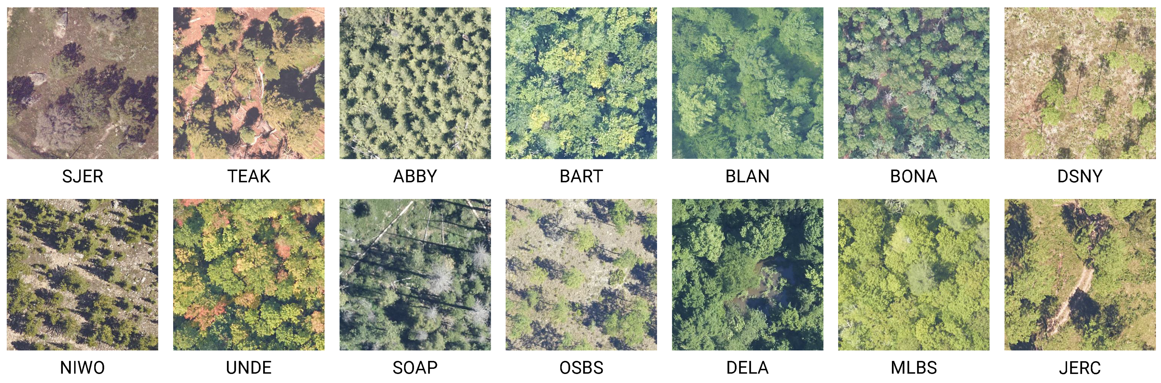
4.2. NeonTreeEvaluation Dataset

We also evaluate the models using NeonTreeEvaluation Dataset [16], which is collected from 22 sites across the United States by multiple types of sensors. The forest types vary in different sites. (Examples are shown in Figure 8). In this work, we only use the fully labeled RGB data, as follows: (1) A test set of 194 images containing 6634 annotated trees. The size of each image is 400 × 400 pixels and corresponds to a 40 m × 40 m region in the real world. (2) A training set including 15 much larger images, containing 17,790 annotated trees. We crop them into 3395 400 × 400 training images as consistent with the test images.

5. Experiments

5.1. Evaluation Metric

By following the works for crowd density estimation, we evaluate different methods for tree counting using Mean absolute error (MAE) and Root Mean Squared Error (RMSE), which are defined as follows:
M A E = 1 N i = 1 N z i z ^ i , R M S E = 1 N i = 1 N z i z ^ i 2
where N is the total number of blocks of in the test set, z i denotes the true number of trees in the ith block, and z ^ i is the predicted number of trees in the ith block inferred by algorithms. For the NeonTreeEvaluation Dataset, a block is simply a test image. For the Yosemite Tree Dataset, we set the block size to 960 × 960 and 4800 × 4800 and report the results.

5.2. Comparison to State-of-Art Methods

We compare DENT with the state-of-the-art methods of different fashions, including density-based methods and detection-based methods. The tested density-based methods include fully convolutional networks originally designed for segmentation and crowd counting. The tested detection-based methods include one-stage and two-stage, anchor-based and anchor-free detectors. For the methods of Faster-RCNN, RetinaNet, YOLOv3, CenterNet, CSRNet, SANet, and CANNet we use their official implementations. For the other methods, we use their third-party open-source implementations.
The results are shown in Table 1 and Table 2. The two heads of DENT, i.e., the DMG and the tree counter, achieve a closed performance. On the Yosemite Dataset, they are nearly on par with CANNet and outperform the other state-of-the-art methods in terms of MAE and RMSE for every test region and block size setting. On the cross-site NeonTreeEvaluation Dataset, they significantly outperform all the other methods.

5.3. Technical Details

We implement DENT using PyTorch [55]. The DMG is based on the ResNet18 released in the PyTorch model zoo. The bert encoder is based on the BERT model released in the Hugging Face (https://huggingface.co/) (accessed on 31 December 2021) model zoo. We set d model = 512 and h = 8 for the multi-head attention. The dimension of the intermediate layer in the feed-forward networks is 2048. Under this setting, the DENT model has 17.82 M parameters. The standard deviation of the Gaussian kernel for density map generation is σ = 15 .
On the Yosemite Tree Dataset, we crop 320 × 320 subimages from the study areas for training and testing. While on the NeonTreeEvaluation Dataset, as the test set are officially provided as 400 × 400 images, we crop 400 × 400 subimages for training from the large training images. As the downsampling rate of the whole DENT is 32, we pad the input images with zero values to 416 × 416 in both the training phase and test phase. The batch sizes we used to train DENT on Yosemite Tree Dataset and NeonTreeEvaluation Dataset are 48 and 32 respectively. Except for those mentioned above, we use the same setting to train DENT on the two datasets.
Pretraining and initialization. The ResNet in the Multi-RF network is pre-trained on the ImageNet dataset [56,57]. All the other components of DENT are learned from scratch. All the parameters of the transformer are initialized with Xavier [58]. The token type embeddings are initialized using a normal distribution.
Loss. The total loss during training is the weighted sum of the losses of the DMG and tree counter:
L = L DMG + λ L CNT
where λ is a weighting factor to balance the losses of the two heads. In our experiments, we use λ = 1 by default.
Optimizer. We use Adam [59] to minimize the loss for a total of 300 epochs without weight decay. The initial learning rate is 10 5 for the first 100 epochs. And then we apply a learning rate decay by a factor of 0.5 for every 50 epochs. We also apply gradient clipping to stabilize the training. The max norm of the gradients is set to 0.1.
Regularization and Data Augmentation. For reducing overfitting, dropout and random-flip are applied. Specifically, a dropout of 0.1 is added before each Add&Norm layer in the transformer encoder. The training images along with the target tree density map are randomly flipped horizontally and/or vertically.

5.4. Ablation Study

To evaluate the effects of the Multi-RF CNN and the transformer layers, ablation experiments are done on the test set (union of Region A and Region C) of Yosemite Tree Dataset for 960 × 960 blocks. The results are provided in Table 3. We start from a ResNet18 without a transformer. The output is projected to a single-channel linearly using a 1 × 1 convolutional layer. Interestingly this baseline already achieves lower errors compared with some existing methods (Table 1). After Adding two extra paths to the ResNet18 to get a Multi-RF network, the counting errors are lowered (The third row in Table 1). Adding two transformer layers as encoder make performance gain on both ResNet18 and Multi-RF network. We also try different numbers of transformer layers. Two layers work best in our experiments. More layers worsen the results and take a longer training time to converge.

5.5. Inference Time

To demonstrate the computational efficiency of DENT we test it on the whole 19,200 × 38,400 study area and report the inference time. The tests are done with a single NVIDIA Tesla V100 SXM2 GPU with CUDA 11.3. Every neural layer runs in native PyTorch with batch size = 1 in the default FP32 precision. We run 10 times for each case and report the average. The inference time of our basic implementation is 47.8 s.
Faster version. Due to the shift-invariance of convolution, when a study area is scanned by the Multi-RF CNN, the size of the scan window (input size) does not affect the final feature map. (This is true only when every layer in the backbone has padding size = 0. And beware that if padding size = 0 is used at test time, it should be used at training time as well to avoid accuracy drop.) We adopt a two-stage inference mode to improve the GPU utilization and lower the time cost: At the first stage, the backbone takes in a larger input image (The resolution is still 11.8 cm GSD. But each input image covers a larger area in the real world.) and generates a larger feature map. At the second stage, the transformer along with the DMG and the tree counter scans the feature map using its original input size. We test this strategy with a 4800 × 4800 input size for the Multi-RF CNN, the inference time is shortened to 16.0 s. When the DMG is pruned as discussed in Section 3.4, the inference time can be further shortened to 11.5 s. Even further improvement is possible with tricks like batch processing and low precision inference but beyond the scope of this paper. A comparison of these different implementations of DENT and the state-of-art object detectors in terms of inference time is shown in Table 4.

6. Conclusions and Future Work

We presented a deep neural regressor, DENT, based on CNN and transformer for tree counting in aerial images. We built a large benchmark dataset, Yosemite Tree Dataset, to evaluate different tree counting algorithms. We also used an existing cross-site dataset to test the robustness of the methods. Our approach achieved competitive results and outperformed the state-of-art methods. The ablation study further supported the effectiveness of the design.
With the advancement of drones, aerial imagery is becoming more and more affordable. However, due to the limited visual field, the captured photos need to be stitched to create the whole picture of a large study field. This procedure can be laborious. For this reason, an accurate video-based tree counting algorithm would be more automatic and appealing. The emerging applications of video-based density estimation methods for crowd counting inspired us. We will explore video-based tree counting algorithms in future work.

Author Contributions

Methodology, Data Curation, and Software, G.C.; Supervision, Y.S. All authors have read and agreed to the published version of the manuscript.

Funding

This research received no external funding.

Conflicts of Interest

The author declares no conflict of interest.

References

  1. Krizhevsky, A.; Sutskever, I.; Hinton, G.E. ImageNet classification with deep convolutional neural networks. In Proceedings of the 25th International Conference on Neural Information Processing Systems, NIPS’12, Lake Tahoe, NV, USA, 3–6 December 2012; Curran Associates Inc.: Red Hook, NY, USA, 2012; Volume 1, pp. 1097–1105. [Google Scholar]
  2. Simonyan, K.; Zisserman, A. Very deep convolutional networks for large-scale image recognition. In Proceedings of the International Conference on Learning Representations, San Diego, CA, USA, 7–9 May 2015. [Google Scholar]
  3. He, K.; Zhang, X.; Ren, S.; Sun, J. Deep residual learning for image recognition. In Proceedings of the 2016 IEEE Conference on Computer Vision and Pattern Recognition (CVPR), Las Vegas, NV, USA, 27–30 June 2016; pp. 770–778. [Google Scholar]
  4. Szegedy, C.; Liu, W.; Jia, Y.; Sermanet, P.; Reed, S.; Anguelov, D.; Erhan, D.; Vanhoucke, V.; Rabinovich, A. Going deeper with convolutions. In Proceedings of the 2015 IEEE Conference on Computer Vision and Pattern Recognition (CVPR), Boston, MA, USA, 7–12 June 2015; pp. 1–9. [Google Scholar]
  5. Szegedy, C.; Vanhoucke, V.; Ioffe, S.; Shlens, J.; Wojna, Z. Rethinking the inception architecture for computer vision. In Proceedings of the 2016 IEEE Conference on Computer Vision and Pattern Recognition (CVPR), Las Vegas, NV, USA, 27–30 June 2016; pp. 2818–2826. [Google Scholar]
  6. Ren, S.; He, K.; Girshick, R.; Sun, J. Faster R-CNN: Towards real-time object detection with region proposal networks. In Proceedings of the 28th International Conference on Neural Information Processing Systems, NIPS’15, Montreal, QC, Canada, 7–12 December 2015; MIT Press: Cambridge, MA, USA, 2015; Volume 1, pp. 91–99. [Google Scholar]
  7. Liu, W.; Anguelov, D.; Erhan, D.; Szegedy, C.; Reed, S.; Fu, C.Y.; Berg, A.C. SSD: Single shot multiBox detector. In European Conference on Computer Vision (ECCV), Proceedings of the 14th European Conference, Amsterdam, The Netherlands, 11–14 October 2016; Leibe, B., Matas, J., Sebe, N., Welling, M., Eds.; Springer International Publishing: Cham, Switzerland, 2016; pp. 21–37. [Google Scholar]
  8. Lin, T.Y.; Goyal, P.; Girshick, R.; He, K.; Dollár, P. Focal loss for dense object detection. In Proceedings of the IEEE International Conference on Computer Vision (ICCV), Venice, Italy, 22–29 October 2017; pp. 2999–3007. [Google Scholar]
  9. Redmon, J.; Farhadi, A. Yolov3: An incremental improvement. arXiv 2018, arXiv:1804.02767. [Google Scholar]
  10. Zhou, X.; Wang, D.; Krähenbühl, P. Objects as points. arXiv 2019, arXiv:1904.07850. [Google Scholar]
  11. Carion, N.; Massa, F.; Synnaeve, G.; Usunier, N.; Kirillov, A.; Zagoruyko, S. End-to-end object detection with transformers. In European Conference on Computer Vision (ECCV), Proceedings of the 16th European Conference, Glasgow, UK, 23–28 August 2020; Vedaldi, A., Bischof, H., Brox, T., Frahm, J.M., Eds.; Springer International Publishing: Cham, Switzerland, 2020; pp. 213–229. [Google Scholar]
  12. Mubin, N.A.; Nadarajoo, E.; Shafri, H.Z.M.; Hamedianfar, A. Young and mature oil palm tree detection and counting using convolutional neural network deep learning method. Int. J. Remote Sens. 2019, 40, 7500–7515. [Google Scholar] [CrossRef]
  13. Li, W.; Fu, H.; Yu, L.; Cracknell, A. Deep learning based oil palm tree detection and counting for high-resolution remote sensing images. Remote Sens. 2017, 9, 22. [Google Scholar] [CrossRef] [Green Version]
  14. Xia, M.; Li, W.; Fu, H.; Yu, L.; Dong, R.; Zheng, J. Fast and robust detection of oil palm trees using high-resolution remote sensing images. In Automatic Target Recognition XXIX; Hammoud, R.I., Overman, T.L., Eds.; International Society for Optics and Photonics, SPIE: Bellingham, WA, USA, 2019; Volume 10988, pp. 65–73. [Google Scholar]
  15. Machefer, M.; Lemarchand, F.; Bonnefond, V.; Hitchins, A.; Sidiropoulos, P. Mask R-CNN Refitting Strategy for Plant Counting and Sizing in UAV Imagery. Remote Sens. 2020, 12, 3015. [Google Scholar] [CrossRef]
  16. Weinstein, B.G.; Marconi, S.; Bohlman, S.; Zare, A.; White, E. Individual tree-crown detection in RGB imagery using semi-supervised deep learning neural networks. Remote Sens. 2019, 11, 1309. [Google Scholar] [CrossRef] [Green Version]
  17. Roslan, Z.; Awang, Z.; Husen, M.N.; Ismail, R.; Hamzah, R. Deep learning for tree crown detection in tropical forest. In Proceedings of the 2020 14th International Conference on Ubiquitous Information Management and Communication (IMCOM), Taichung, Taiwan, 3–5 January 2020; pp. 1–7. [Google Scholar]
  18. Zheng, J.; Li, W.; Xia, M.; Dong, R.; Fu, H.; Yuan, S. Large-scale oil palm tree detection from high-resolution remote sensing images using faster-rcnn. In Proceedings of the IGARSS 2019-2019 IEEE International Geoscience and Remote Sensing Symposium, Yokohama, Japan, 28 July–2 August 2019; pp. 1422–1425. [Google Scholar]
  19. Zhang, Y.; Zhou, D.; Chen, S.; Gao, S.; Ma, Y. Single-image crowd counting via multi-column convolutional neural network. In Proceedings of the 2016 IEEE Conference on Computer Vision and Pattern Recognition (CVPR), Las Vegas, NV, USA, 27–30 June 2016; pp. 589–597. [Google Scholar]
  20. Sam, D.B.; Surya, S.; Babu, R.V. Switching convolutional neural network for crowd counting. In Proceedings of the 2017 IEEE Conference on Computer Vision and Pattern Recognition (CVPR), Honolulu, HI, USA, 21–26 July 2017; pp. 4031–4039. [Google Scholar]
  21. Li, Y.; Zhang, X.; Chen, D. CSRNet: Dilated convolutional neural networks for understanding the highly congested scenes. In Proceedings of the 2018 IEEE/CVF Conference on Computer Vision and Pattern Recognition (CVPR), Salt Lake City, UT, USA, 18–23 June 2018; pp. 1091–1100. [Google Scholar]
  22. Cao, X.; Wang, Z.; Zhao, Y.; Su, F. Scale aggregation network for accurate and efficient crowd counting. In Proceedings of the European Conference on Computer Vision (ECCV), Munich, Germany, 8–14 September 2018; Ferrari, V., Hebert, M., Sminchisescu, C., Weiss, Y., Eds.; Springer International Publishing: Cham, Switzerland, 2018; pp. 757–773. [Google Scholar]
  23. Liu, W.; Salzmann, M.; Fua, P. Context-aware crowd counting. In Proceedings of the 2019 IEEE/CVF Conference on Computer Vision and Pattern Recognition (CVPR), Long Beach, CA, USA, 15–20 June 2019; pp. 5094–5103. [Google Scholar]
  24. Djerriri, K.; Ghabi, M.; Karoui, M.S.; Adjoudj, R. Palm trees counting in remote sensing imagery using regression convolutional neural network. In Proceedings of the IGARSS 2018-2018 IEEE International Geoscience and Remote Sensing Symposium, Valencia, Spain, 22–27 July 2018; pp. 2627–2630. [Google Scholar]
  25. Yao, L.; Liu, T.; Qin, J.; Lu, N.; Zhou, C. Tree counting with high spatial-resolution satellite imagery based on deep neural networks. Ecol. Indic. 2021, 125, 107591. [Google Scholar] [CrossRef]
  26. Weinstein, B.G.; Marconi, S.; Bohlman, S.A.; Zare, A.; White, E.P. Cross-site learning in deep learning RGB tree crown detection. Ecol. Inform. 2020, 56, 101061. [Google Scholar] [CrossRef]
  27. Vaswani, A.; Shazeer, N.; Parmar, N.; Uszkoreit, J.; Jones, L.; Gomez, A.N.; Kaiser, L.; Polosukhin, I. Attention is all you need. In Proceedings of the 31st International Conference on Neural Information Processing Systems, NIPS’17, Long Beach, CA, USA, 4–9 December 2017; Curran Associates Inc.: Red Hook, NY, USA, 2017; pp. 6000–6010. [Google Scholar]
  28. Dosovitskiy, A.; Beyer, L.; Kolesnikov, A.; Weissenborn, D.; Zhai, X.; Unterthiner, T.; Dehghani, M.; Minderer, M.; Heigold, G.; Gelly, S.; et al. An Image is Worth 16×16 Words: Transformers for Image Recognition at Scale. In Proceedings of the International Conference on Learning Representations, Virtual, 3–7 May 2021. [Google Scholar]
  29. Mekhalfi, M.L.; Nicolò, C.; Bazi, Y.; Rahhal, M.M.A.; Alsharif, N.A.; Maghayreh, E.A. Contrasting YOLOv5, Transformer, and EfficientDet Detectors for Crop Circle Detection in Desert. IEEE Geosci. Remote Sens. Lett. 2022, 19, 1–5. [Google Scholar] [CrossRef]
  30. Bazi, Y.; Bashmal, L.; Rahhal, M.M.A.; Dayil, R.A.; Ajlan, N.A. Vision Transformers for Remote Sensing Image Classification. Remote Sens. 2021, 13, 516. [Google Scholar] [CrossRef]
  31. Ronneberger, O.; Fischer, P.; Brox, T. U-net: Convolutional networks for biomedical image segmentation. In International Conference on Medical Image Computing and Computer-Assisted Intervention (MICCAI), Proceedings of the 18th International Conference, Munich, Germany, 5–9 October 2015; Springer International Publishing: Cham, Switzerland, 2015; pp. 234–241. [Google Scholar]
  32. Rowley, H.; Baluja, S.; Kanade, T. Human face detection in visual scenes. In Advances in Neural Information Processing Systems; Touretzky, D., Mozer, M.C., Hasselmo, M., Eds.; MIT Press: Cambridge, MA, USA, 1996; Volume 8. [Google Scholar]
  33. Viola, P.; Jones, M. Rapid object detection using a boosted cascade of simple features. In Proceedings of the 2001 IEEE Computer Society Conference on Computer Vision and Pattern Recognition (CVPR), Kauai, HI, USA, 8–14 December 2001; Volume 1, pp. 511–518. [Google Scholar]
  34. Dalal, N.; Triggs, B. Histograms of oriented gradients for human detection. In Proceedings of the 2005 IEEE Computer Society Conference on Computer Vision and Pattern Recognition (CVPR), San Diego, CA, USA, 20–26 June 2005; Volume 1, pp. 886–893. [Google Scholar]
  35. Felzenszwalb, P.F.; Girshick, R.B.; McAllester, D.; Ramanan, D. Object detection with discriminatively trained part-based models. IEEE Trans. Pattern Anal. Mach. Intell. 2009, 32, 1627–1645. [Google Scholar] [CrossRef] [Green Version]
  36. Harzallah, H.; Jurie, F.; Schmid, C. Combining efficient object localization and image classification. In Proceedings of the 2009 IEEE 12th International Conference on Computer Vision (ICCV), Kyoto, Japan, 27 September–4 October 2009; pp. 237–244. [Google Scholar]
  37. Lowe, D. Object recognition from local scale-invariant features. In Proceedings of the Seventh IEEE International Conference on Computer Vision (ICCV), Corfu, Greece, 20–25 September 1999; Volume 2, pp. 1150–1157. [Google Scholar]
  38. Pollock, R. The Automatic Recognition of Individual Trees in Aerial Images of Forests Based on a Synthetic Tree Crown Image Model. Ph.D. Thesis, University of British Columbia, Vancouver, BC, Canada, 1996. [Google Scholar]
  39. Larsen, M.; Rudemo, M. Using ray-traced templates to find individual trees in aerial photographs. In Proceedings of the Scandinavian Conference on Image Analysis, Lappenranta, Finland, 9–11 June 1997; Volume 2, pp. 1007–1014. [Google Scholar]
  40. Vibha, L.; Shenoy, P.D.; Venugopal, K.; Patnaik, L. Robust technique for segmentation and counting of trees from remotely sensed data. In Proceedings of the 2009 IEEE International Advance Computing Conference, Patiala, India, 6–7 March 2009; pp. 1437–1442. [Google Scholar]
  41. Hung, C.; Bryson, M.; Sukkarieh, S. Vision-based shadow-aided tree crown detection and classification algorithm using imagery from an unmanned airborne vehicle. In Proceedings of the 34th International Symposium for Remote Sensing of the Environment (ISRSE), Sydney, Australia, 10–15 April 2011. [Google Scholar]
  42. Manandhar, A.; Hoegner, L.; Stilla, U. Palm tree detection using circular autocorrelation of polar shape matrix. ISPRS Ann. Photogramm. Remote Sens. Spat. Inf. Sci. 2016, 3, 465–472. [Google Scholar] [CrossRef] [Green Version]
  43. Wang, Y.; Zhu, X.; Wu, B. Automatic detection of individual oil palm trees from UAV images using HOG features and an SVM classifier. Int. J. Remote Sens. 2019, 40, 7356–7370. [Google Scholar] [CrossRef]
  44. Li, W.; Fu, H.; Yu, L. Deep convolutional neural network based large-scale oil palm tree detection for high-resolution remote sensing images. In Proceedings of the 2017 IEEE International Geoscience and Remote Sensing Symposium (IGARSS), Fort Worth, TX, USA, 23–28 July 2017; pp. 846–849. [Google Scholar]
  45. Li, W.; Dong, R.; Fu, H.; Yu, L. Large-scale oil palm tree detection from high-resolution satellite images using two-stage convolutional neural networks. Remote Sens. 2019, 11, 11. [Google Scholar] [CrossRef] [Green Version]
  46. Huang, G.; Liu, Z.; Maaten, L.V.D.; Weinberger, K.Q. Densely connected convolutional networks. In Proceedings of the 2017 IEEE Conference on Computer Vision and Pattern Recognition (CVPR), Honolulu, HI, USA, 21–26 July 2017; pp. 2261–2269. [Google Scholar]
  47. Freudenberg, M.; Nölke, N.; Agostini, A.; Urban, K.; Wörgötter, F.; Kleinn, C. Large scale palm tree detection in high resolution satellite images using U-Net. Remote Sens. 2019, 11, 312. [Google Scholar] [CrossRef] [Green Version]
  48. Miyoshi, G.T.; Arruda, M.d.S.; Osco, L.P.; Marcato Junior, J.; Gonçalves, D.N.; Imai, N.N.; Tommaselli, A.M.G.; Honkavaara, E.; Gonçalves, W.N. A novel deep learning method to identify single tree species in UAV-based hyperspectral images. Remote Sens. 2020, 12, 1294. [Google Scholar] [CrossRef] [Green Version]
  49. Araujo, A.; Norris, W.; Sim, J. Computing receptive fields of convolutional neural networks. Distill 2019, 4, e21. [Google Scholar] [CrossRef]
  50. Ba, J.; Kiros, J.R.; Hinton, G.E. Layer normalization. arXiv 2016, arXiv:1607.06450. [Google Scholar]
  51. Parmar, N.J.; Vaswani, A.; Uszkoreit, J.; Kaiser, L.; Shazeer, N.; Ku, A.; Tran, D. Image transformer. In Proceedings of the International Conference on Machine Learning (ICML), Stockholm, Sweden, 10–15 July 2018. [Google Scholar]
  52. Devlin, J.; Chang, M.W.; Lee, K.; Toutanova, K. Bert: Pre-training of deep bidirectional transformers for language understanding. arXiv 2018, arXiv:1810.04805. [Google Scholar]
  53. Lei, J.; Wang, L.; Shen, Y.; Yu, D.; Berg, T.L.; Bansal, M. Mart: Memory-augmented recurrent transformer for coherent video paragraph captioning. arXiv 2020, arXiv:2005.05402. [Google Scholar]
  54. Badrinarayanan, V.; Kendall, A.; Cipolla, R. Segnet: A deep convolutional encoder-decoder architecture for image segmentation. IEEE Trans. Pattern Anal. Mach. Intell. 2017, 39, 2481–2495. [Google Scholar] [CrossRef] [PubMed]
  55. Paszke, A.; Gross, S.; Chintala, S.; Chanan, G.; Yang, E.; DeVito, Z.; Lin, Z.; Desmaison, A.; Antiga, L.; Lerer, A. Automatic differentiation in pytorch. In Proceedings of the Neural Information Processing Systems Workshop, Long Beach, CA, USA, 4–9 December 2017. [Google Scholar]
  56. Deng, J.; Dong, W.; Socher, R.; Li, L.J.; Li, K.; Li, F.-F. Imagenet: A large-scale hierarchical image database. In Proceedings of the 2009 IEEE Conference on Computer Vision and Pattern Recognition, Miami, FL, USA, 20–25 June 2009; pp. 248–255. [Google Scholar]
  57. Russakovsky, O.; Deng, J.; Su, H.; Krause, J.; Satheesh, S.; Ma, S.; Huang, Z.; Karpathy, A.; Khosla, A.; Bernstein, M.; et al. ImageNet large scale visual recognition challenge. Int. J. Comput. Vis. (IJCV) 2015, 115, 211–252. [Google Scholar] [CrossRef] [Green Version]
  58. Glorot, X.; Bengio, Y. Understanding the difficulty of training deep feedforward neural networks. In JMLR Workshop and Conference Proceedings, Proceedings of the Thirteenth International Conference on Artificial Intelligence and Statistics, Sardinia, Italy, 13–15 May 2010; PMLR: New York City, NY, USA, 2010; pp. 249–256. [Google Scholar]
  59. Kingma, D.P.; Ba, J. Adam: A method for stochastic optimization. arXiv 2014, arXiv:1412.6980. [Google Scholar]
Figure 1. Comparison among different types of annotations for tree counting methods. (a) The original image. (b) Bounding boxes. (c) Keypoints. (d) Tree density map.
Remotesensing 14 00476 g001
Figure 2. The architecture of the proposed DENT Network. (a) Visual features are extracted using a Multi-Receptive Field convolutional network (Multi-RF CNN). (b) Positional encoding and token type embedding are applied to the visual features. The visual features are flattened as a sequence [ f 0 , f 1 , . . . , f L ] . (c) f cnt , the embedding of CNT token, works as a count query. (d) The visual feature sequence and the count query are concatenated as the input of the transformer encoder. On top of the transformer encoder, there are two heads: A Density Map Generator (DMG) predicts the density of objects at different positions. A counter predicts the count of the objects in the whole input image.
Remotesensing 14 00476 g002
Figure 3. Architecture of the proposed Multi-Receptive Field network. This CNN has three different paths to output feature maps, each has its own receptive field. (a) The receptive fields of Path A and C are visualized as boxes. (b) The backbone is built using a residual convolutional block. (c) The three paths diverge from Block 2. Path B contains two 1 × 1 conv. layers. Path C contains only an average pooling layer. (d) The output feature maps are concatenated along the channel axis to compose the final output.
Remotesensing 14 00476 g003
Figure 4. (a) The architecture of an transformer encoder layer. (b) The architecture of the multi-head attention sublayer.
Remotesensing 14 00476 g004
Figure 5. A comparison between the granularities of the DMG and the tree counter. (a) An example image from a 4800 × 4800 region, which is 566 m × 566 m in real world. (b) The corresponding 150 × 150 desity map generated by DMG. (c) The corresponding 15 × 15 coarser density map generated using the tree counter.
Remotesensing 14 00476 g005
Figure 6. (a) The study area of the Yosemite Tree Dataset. (b) Example images cropped from different locations of the dataset.
Remotesensing 14 00476 g006
Figure 7. Histograms of tree counts of Yosemite Tree Dataset.
Remotesensing 14 00476 g007
Figure 8. Examples of the test images in NeonTreeEvaluation Dataset [16]. The four-letter captions under the images are abbreviations of the site names. The forest types vary across different sites.
Remotesensing 14 00476 g008
Table 1. Counting errors of different approaches on Yosemite Tree Dataset. The bold numbers are the lowest values in each column.
Block Size: 960 × 960Block Size: 4800 × 4800
113 m × 113 m in Real World566 m × 566 m in Real World
Region ARegion CRegion ARegion C
MethodMAERMSEMAERMSEMAERMSEMAERMSE
UNet [31]16.320.712.917.7318.5367.0203.8228.0
MCNN [19]19.725.316.821.0311.0371.1283.3378.0
MCNN (End-to-end) [19]21.827.618.422.7388.2453.6239.4286.5
SwitchCNN [20]17.222.214.818.5271.1317.9175.7212.2
SegNet [54]12.717.015.919.4270.6299.7209.8228.5
CSRNet [21]20.926.319.124.6287.0364.7295.3301.3
SANet [22]18.423.517.622.1272.1344.6285.6297.9
CANNet [23]10.813.812.016.2122.6161.1130.2159.5
Faster-RCNN-ResNet50 [6]13.918.115.020.0260.2269.7237.0278.0
Faster-RCNN-ResNet101 [6]13.417.415.920.9235.9256.6240.6285.2
RetinaNet-ResNet50 [8]14.318.115.018.6224.1248.7187.5240.0
RetinaNet-ResNet101 [8]16.020.216.221.1290.7317.2233.2301.8
YOLOv3 [9]17.322.615.620.1353.2383.6256.9286.9
CenterNet-DLA34 [10]14.920.714.619.0344.9398.0250.0299.9
CenterNet-ResNet50 [10]13.717.513.717.4311.1335.3237.9257.8
CenterNet-ResNet101 [10]12.116.213.417.2237.6271.4212.0241.4
DENT-DMG10.713.711.916.5148.7163.9123.9158.3
DENT-CNT10.713.712.016.6140.6154.4133.7169.3
Table 2. Counting errors of different approaches on NeonTreeEvaluation Dataset. The bold numbers are the lowest values in each column.
MethodMAERMSE
UNet [31]34.756.4
MCNN [19]14.724.7
MCNN End-to-end [19]15.525.7
SwitchCNN [20]15.225.1
SegNet [54]28.947.5
CSRNet [21]33.952.2
SANet [22]18.430.1
CANNet [23]14.623.1
Faster-RCNN-ResNet50 [6]11.115.7
Faster-RCNN-ResNet101 [6]11.918.2
RetinaNet-ResNet50 [8]10.915.9
RetinaNet-ResNet101 [8]12.016.8
YOLOv3 [9]15.231.8
CenterNet-DLA34 [10]10.217.2
CenterNet-ResNet50 [10]13.023.5
CenterNet-ResNet101 [10]12.520.4
DENT-DMG7.512.3
DENT-CNT7.612.2
Table 3. Comparison of models with different CNNs and number of transformer layers on Yosemite Tree Dataset for block size 960 × 960. The models are tested on the union of Region A and Region C. When #transformer layers = 0 , the CNN features are linearly projected to the predicted density map, otherwise, the density map is generated by DMG. The bold numbers are the lowest values in each column.
Visual Feature Extractor#Transformer LayersMAERMSE
ResNet18013.417.7
ResNet18212.816.9
Multi-RF013.017.0
Multi-RF112.016.5
Multi-RF211.315.2
Multi-RF311.816.7
Table 4. Inference time comparison on the Yosemite Tree Counting Dataset. The bold numbers are the lowest values in each column.
MethodBackboneInference Time (Seconds)
Faster-RCNN [6]ResNet50290.9
RetinaNet [8]ResNet50270.3
YOLOv3 [9]Darknet53163.2
CenterNet [10]DLA3461.5
DENTResNet1847.8
DENT-fasterResNet1816.0
DENT-faster without DMGResNet1811.5
Publisher’s Note: MDPI stays neutral with regard to jurisdictional claims in published maps and institutional affiliations.

