Article

Grassland Phenology Response to Climate Conditions in Biobio, Chile from 2001 to 2020

by
Marcelo-Alejandro Doussoulin-Guzmán
1,
Fernando-Juan Pérez-Porras
2,
Paula Triviño-Tarradas
2,
Andrés-Felipe Ríos-Mesa
3,
Alfonso García-Ferrer Porras
1 and
Francisco-Javier Mesas-Carrascosa
2,*
1
Department of Animal Production, Faculty of Agronomy, Universidad de Concepción, Chillán 3812120, Chile
2
Department of Graphic Engineering and Geomatics, University of Cordoba, Campus de Rabanales, Crta. IV, km. 396, E-14071 Córdoba, Spain
3
Agroindustrial Engineering Faculty, University Pontificia Bolivariana, Medellín 050031, Colombia
*
Author to whom correspondence should be addressed.
Remote Sens. 2022, 14(3), 475; https://doi.org/10.3390/rs14030475
Submission received: 13 December 2021 / Revised: 13 January 2022 / Accepted: 17 January 2022 / Published: 20 January 2022
(This article belongs to the Special Issue Remote Sensing for Agricultural, Environmental and Forestry Policies)

Abstract

:
Plant phenology is affected by climate conditions and therefore provides a sensitive indicator to changes in climate. Studying the evolution and change in plant phenology aids in a better understanding of and predicting changes in ecosystems. Vegetation Indices (VIs) have been recognized for their utility in indicating vegetation activity. Understanding climatic variables and their relationship to VI support the knowledge base of how ecosystems are changing under a new climatic scenario. This study evaluates grassland growth phenology in the Biobio, Chile, biweekly with Moderate Resolution Imaging Spectroradiometer (MODIS) Normalized Difference Vegetation Index (NDVI) time series. Four growth parameters for the six agro-climatic regions were analyzed from 2001 to 2020: start and end of the season, time and value of maximum NDVI. For this purpose, the NDVI time series were smoothed using Savitzky–Golay filtering. In addition, by using monthly gridded database climate data, we studied correlations between phenology markers and rainfall, maximum temperature and minimum temperature. The results show that both the start and end of the growing season did not significantly change; however, all agro-climatic regions grow faster and more vigorously. Thus, climatic conditions in Biobio have become more conducive to grassland growth over the 2001–2020 period.

Graphical Abstract

1. Introduction

Vegetation phenology is the study of biological patterns in plant growth over time, such as germination, flowering, fruiting, lead emergence, etc. Moreover, it examines how these patterns relate to environmental factors, such as rainfall and air temperature, thus providing information about vegetation productivity, carbon reserve and carbon dynamics [1], which, in turn, yields data on the responses and adaptations of vegetation to climate change [2]. Therefore, monitoring vegetation with phenological metrics provides data to track changes in vegetation linked to events such as drought, fire, climate fluctuations or directional climate change [3]. The impact of climate change on vegetation causes variations in the phenological patterns of vegetation such as temporal displacement of phenological cycles, changes in plant morphology, colonization by other species, or even extinction of other species. Thus, these processes generate important indicators in ecosystem functions and species composition [4,5].
Grasslands are widely distributed around the world and play an important role in carbon storage [6], which is a crucial factor in the mitigation of climate change [7]. Grasslands also provide essential resources for animal life and humankind as well as maintain the stability of ecological systems [8]. Grasslands are especially important to food supply as ruminants produce 37% more food, milk and meat than from pig and poultry [9].
As noted above, grassland plant growth is sensitive to regional and global climatic conditions. Previous research has described how grasslands show complex and varied responses to climate change [10,11]. Some studies concluded that warmer springs result in an earlier start of season (SOS) [12,13]. However, if rainfall decreases, increasing temperatures do not have a significant impact on phenology [14]. Due to the varied effects of climate change on grassland phenology, it is important to understand the responses to phenological events.
Changes in vegetation phenology were studied at a global level as well as regionally in areas of Africa [15], Europe [16], the Tibetan Plateau [17] and the northern high latitudes [1]. Results show that the magnitude of these changes varies depending on location, species and the temporal windows analyzed. Changes in phenology are mainly a response to human activity, rainfall, and temperature [18]. Of all the phenological stages, the SOS and the end of the growing season (EOS) are the most sensitive to climate change [19], more specifically to the effects of global warming caused by the increased atmospheric concentration of greenhouse gasses [20] and water availability [21]. At the same time, the sensitivity to rainfall and temperature differs from region to region [22]. The consequence of this is that the estimated long-term trends in phenological changes are different from one location to another and even for the same location. For example, Jeong et al. [23] showed different values of SOS and EOS in the northern hemisphere depending on the temporal window analyzed.
The two approaches, ground observations and earth observation (EO), can be, respectively, conducted to monitor vegetation phenology at a small scale [24,25] or at a large scale [26,27]. The former provides highly accurate and detailed species-specific phenological information, which is conducted through (a) visual observation of the states of the plant life cycle [24], (b) gas exchange measurement [28] or, (c) on-ground near-spectral measurements [29]. However, ground observations are inefficient, time-limited and expensive [30]. Despite these disadvantages, ground observations are very useful in precision agriculture for crop-specific phenological monitoring as they provide information for crop management such as irrigation, fertilization, and other such practices. On the other hand, EO images from sensors onboard satellite platforms offer vegetation data derived from various spatial, spectral, radiometric and temporal resolutions [31,32] and have lower costs and better spatial-temporal continuity [20]. However, specific phenological events are not all directly detected, and therefore, vegetation patterns are calculated using Land Surface Phenology (LSP) [33], which is more generalized. Remote phenological studies can be divided into two groups, those which analyze trends in Vegetation Indices (VI) and those that derive the duration of status of phenophases to detect changes in phenological patterns. In both cases, data from remote sensing are obtained through temporal series of vegetation indices (VI), mainly the Normalized Difference Vegetation Index (NDVI) [34,35] and the Enhanced Vegetation Index (EVI) [36,37]. Of all the Earth observation projects, products obtained from Moderate Resolution Imaging Spectroradiometer (MODIS) are the most efficient to develop long-term time series of vegetation phenology [38]. MODIS vegetation products are used to monitor the phenology of forestall [39,40,41] and agricultural [42,43] ecosystems, drought monitoring [44,45] and classify crop species [46].
The process of deriving phenological information from remote sensing data includes three steps: (a) analyzing and improving the quality of VI time series, (b) VI time-series smoothing and, finally, (c) identifying relevant periods such as SOS or EOS [31,47]. Firstly, to reduce noise, such as the presence of clouds and/or shadows, off-nadir viewing effect or other errors, Maximum Value Composite (MVC) is applied to obtain temporally composite data [48]. The outputted VI time-series still includes noise artifacts, making smoothing necessary to minimize these residuals to be more representative [49]. The methods of VI time-series smoothing are classified into three groups: empirical methods [50,51], curve fitting methods [52,53] and data transformation [54]. Finally, phenological metrics extraction methods can be divided into two categories, threshold-based and change detection methods.
The objective of this study was to track phenological changes in Biobio grasslands. The study was carried out with the specific aims: (i) Are there significant differences in the timing of phenological markers? (ii) What climatic variables contribute to them? (iii) Are there any trends in these markers in the 2001–2020 period?

2. Materials and Methods
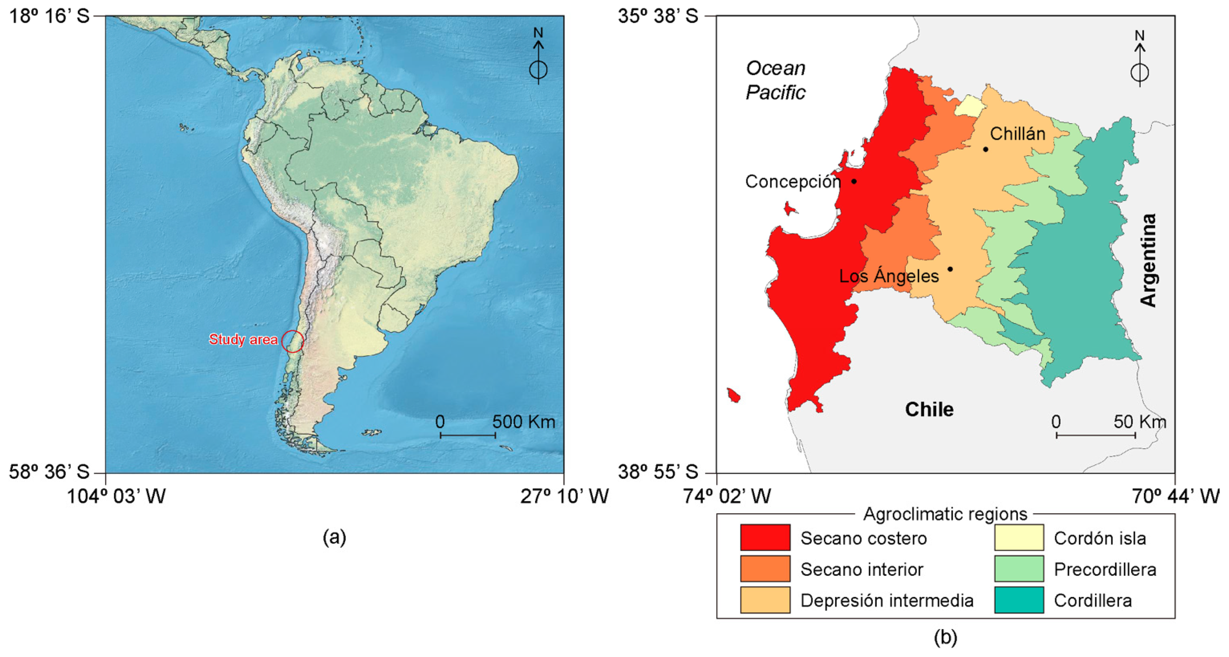
2.1. Study Area

The Biobio Region (Chile) (central coordinates 37°15′ S, 72°30′ W, WGS-84) covers an area of 37,068 km2 (Figure 1a) and is divided in six agro-climatic regions: Secano Costero, Secano Interior, Depresión Intermedia, Cordón Isla, Precordillera and Cordillera (Figure 1b). This region is in a transition area ranging from a warm Mediterranean climate to a humid and temperate climate which makes it sensitive to ecological changes, such as human land use and the effects of climate change. Its bioclimatic variables per Hijmans et al. [55] and through monthly rainfall and temperature values show a total annual range of precipitation from 750 mm to 2000 mm, with the precipitation in the driest month being lower than 35 mm while in wettest month ranging from 150 mm to 350 mm. The temperature in the warmest month is around 25 °C while the coldest month ranges from 0 °C to 7 °C, with the annual mean temperature equal to 10 °C. Most of the region is covered by forest, followed by croplands and grasslands.
The Grasslands in the Biobio region are composed of temperate climate forage species and are classified as natural and sown grassland. Natural grassland yields range from 1.7 to 8.0 tonnes DM × ha−1 × year−1 while sown grassland yields can exceed 15 tonnes, DM × ha−1 × year−1. The natural grasslands are composed of species such as Avena barbata, Bromus mollis, Hordeum murinum, Aira caryophyllea, Paspalum dilatatatum, Brisa minor, Hypochoeris glabra, Erodium cicutarium, Lolium rigidum, Lolium multiflorum, Trifolium glomeratum and Medicago polymorpha; the sown grassland are composed of Lolium perenne, Lolium multiflorum, Dactilis glomerata, Festuca arundinacea, Phalaris aquatica, Trifolium suterráneum, Trifolium michelianum, Trifolium pratense, Trifolium incarnatum, Trifolium repens, Lotus pedunculatus, Medicago sativa and others [56].

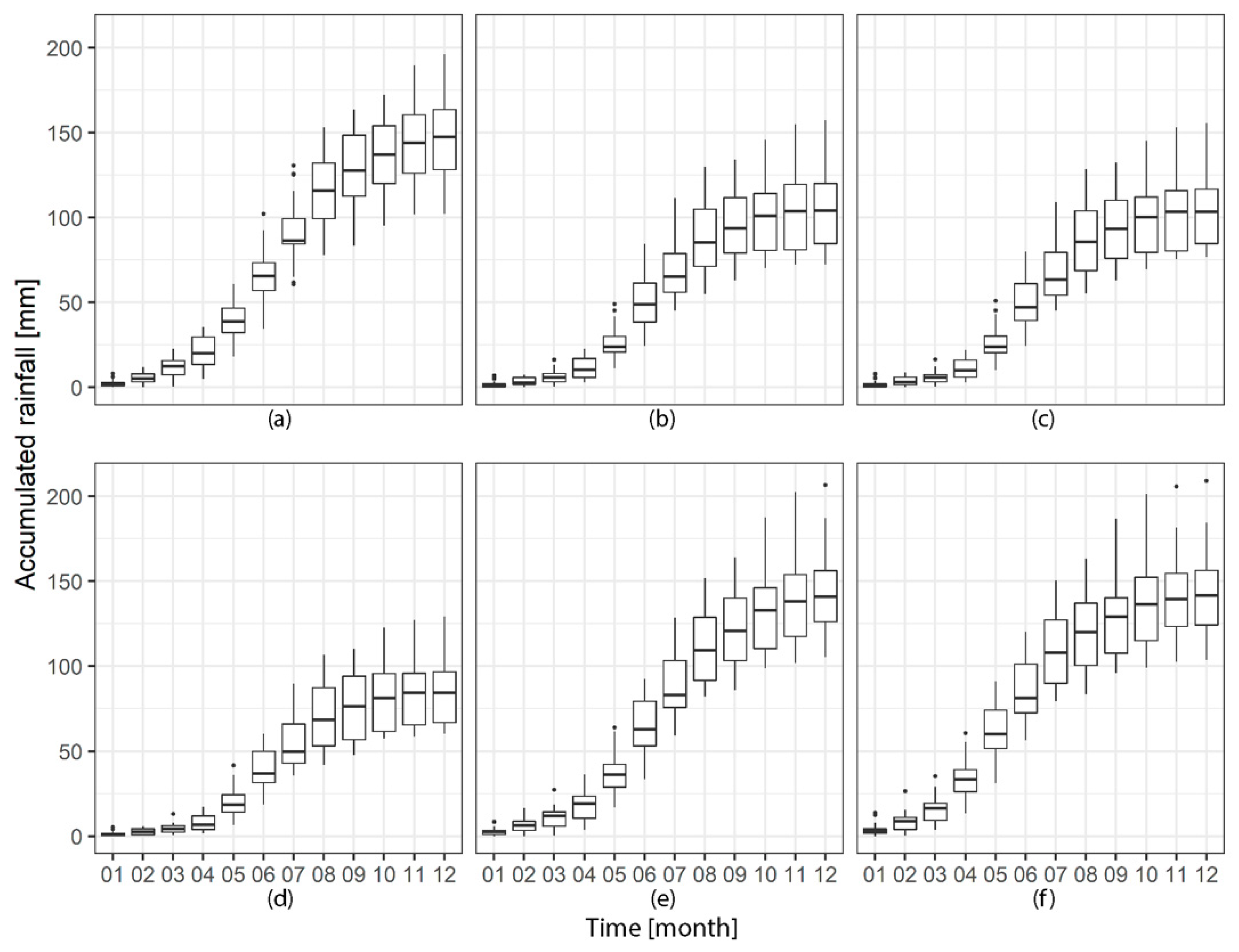
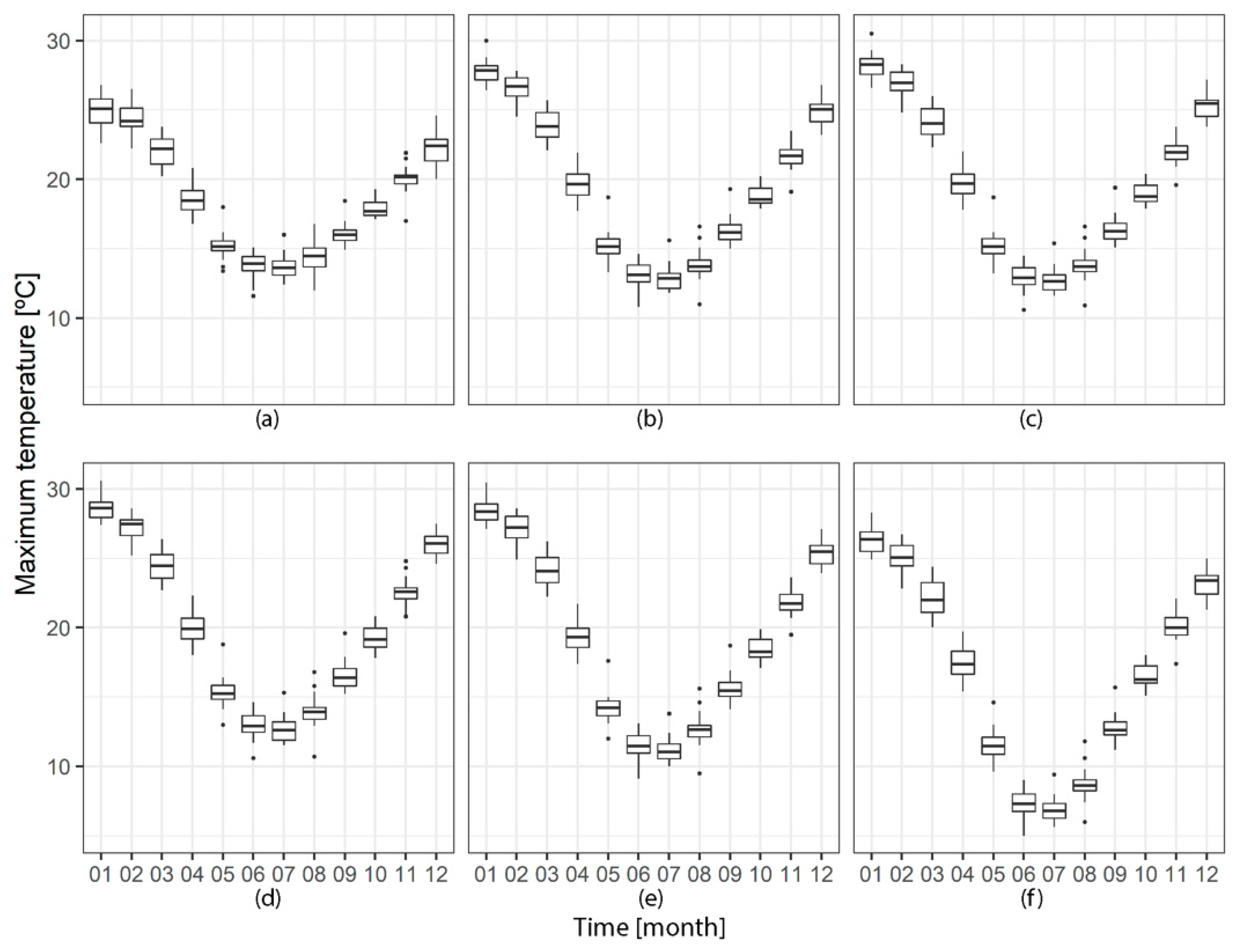
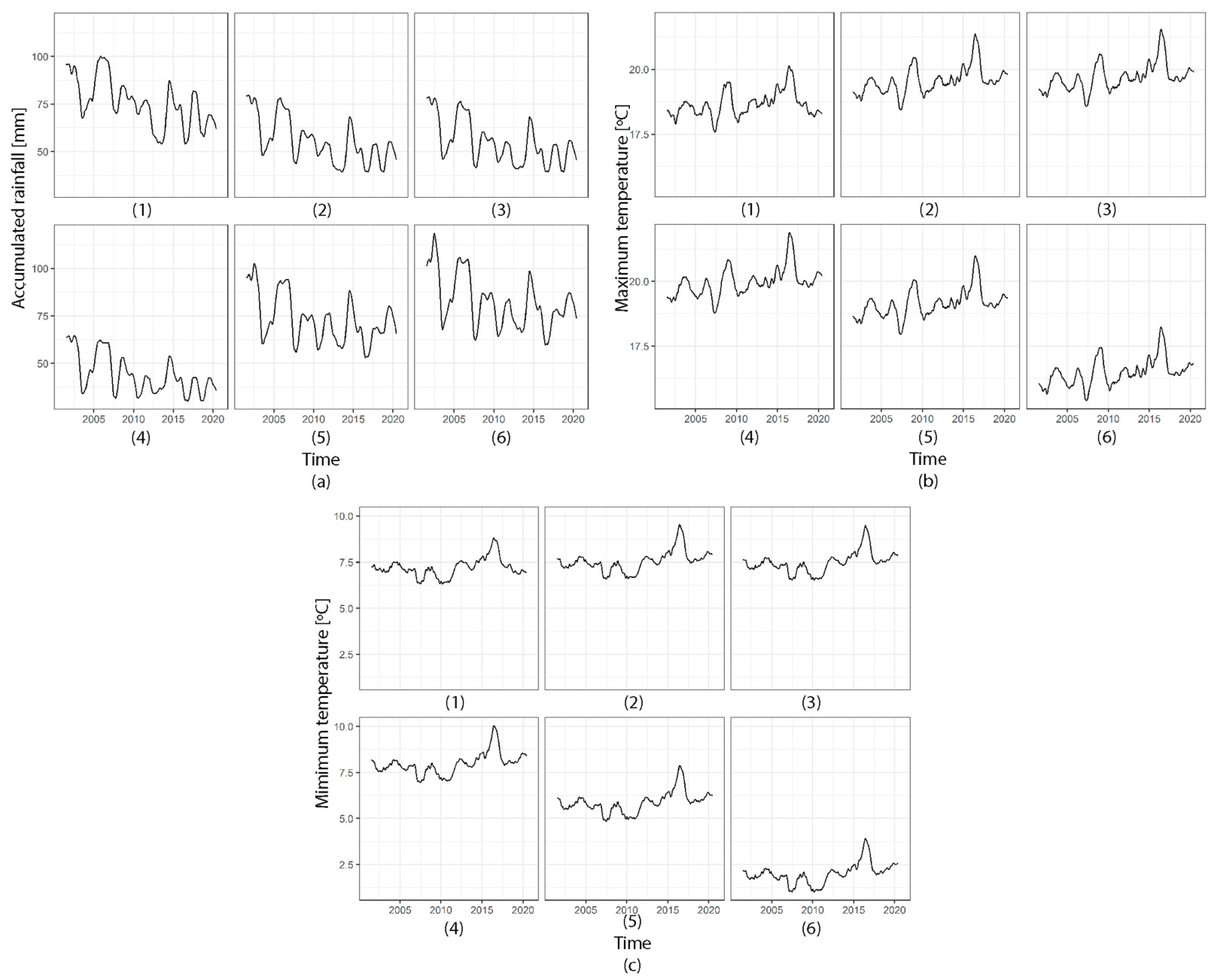
2.2. Evolution of Climatic Variables

This section explains the evolution of the accumulated rainfall and maximum and minimum temperature variables for the six agro-climatic regions of the study area over the period of 2001–2020. The per-year graph densities are shown in Figure 2, which includes the agro-climatic region and climatic variable, the differences between the monthly mean values and their corresponding monthly mean value over the whole time series. In addition, in Appendix A, Figure A1, Figure A2 and Figure A3, represented in the boxplot, graphs the temporal evolution of these variables on a monthly scale for the period studied.
The variations in accumulated rainfall are represented in Figure 2a. When the density graph shifts to the right of 0 in any given year, it means that that year had greater rainfall within the period analyzed. On the other hand, when shifted to the left, that year was dry. In addition, the density graphs in Figure 2a present a binomial distribution, implying an irregular distribution of rainfall between very rainy and very dry periods and presenting similar behaviors across the agro-climatic regions in overall accumulated rainfall. In general terms, between 2001 and 2010, the annual density graphs show a distribution shifted to the right, and therefore accumulated rainfall was higher than the mean of the total period. On the other hand, from 2010 onwards, the curves shifted to the left and, therefore, it was drier. Thus, the accumulated rainfall has been decreasing over the years. There are, however, years with extreme accumulated rainfall values, both due to excess and deficiency. Thus, years such as 2001, 2002, 2005, 2006 and 2014 show higher values than the average of the values recorded between 2001 and 2020, while years such as 2007, 2010, 2012, 2013, 2016 and 2018 had values lower than the average.
In regard to temperature, density graphs shifted to the right of 0 mean warmer years, while those shifted to the left mean colder years. The density graphs with variations of the maximum temperatures with respect to their monthly mean values (Figure 2b) show a tendency to shift to the right with respect to the central value of 0, which indicates an increase in maximum temperatures at the end of the temporal series. The year 2016, in particular, stands out for its increase in maximum temperatures to levels much higher than those in other years within the study period. In addition, it can be seen that the peaks of the density graphs are left at 0 at the beginning of the time series, which means that monthly maximum temperatures were lower than the mean values for 2001–2020. As the time series progresses, the crests of the density graphs move to the right, thus showing increasing maximum temperatures. As with accumulated rainfall, this trend appears across all the agro-climatic regions. Finally, the minimum temperatures, shown in Figure 2c, display the same behavior as the maximum temperatures in such a way that the minimum temperatures at the beginning of the time series were lower than the mean monthly values of the time series analyzed and gradually shift to the right indicating an increase.
The time series of accumulated rainfall, maximum temperature and minimum temperature was decomposed into three components: trend, seasonal and irregular components through an additive model. Each agro-climatic region in Figure 3 shows the trend of the climatic variables analyzed. All of the regions show a downward trend related to accumulated rainfall (Figure 3a). This progressive decrease follows sinusoidal behavior, with very wet years interspersed with drier ones. Moreover, this trend is evident from the beginning of all the agro-climatic series. The Cordón Isla region (Figure 3(a.4)) is the driest of all the regions with a mean value of 860 mm × year−1. On the other hand, Secano Costero, Precordillera, and Cordillera regions are the rainiest with 1478, 1434 and 1431 mm × year−1 average, respectively. Finally, Secano Interior and Depresión Intermedia have a mean accumulated rainfall equal to 1071 and 1059 mm × year−1, respectively. In addition, the Precordillera, Cordillera and Secano Costero regions present the most variability with a standard deviation equal to ±270.9, 268 and 265 mm × year−1. The Cordón Isla, on the other hand, has the least variability with ±214.0 mm × year−1. Lastly, the Secano Interior and Depresión Intermedia regions have a standard deviation equal to ±244 and 231 mm × year−1, respectively. The wettest year was 2002 in all regions, reaching values between 2093 mm in the Cordillera region and 1293 mm in Cordón Isla. The year 2013 was the driest year in the regions of Secano Costero, Secano Interior and Depresión Intermedia, with values equal to 1022, 724 and 767 mm, respectively, while 2007 was the driest year in the regions of Cordón Isla, Precordillera and Cordillera, with annual rainfall values equal to 601, 1055 and 1037 mm.
In the case of temperatures, both maximum (Figure 3b) and minimum (Figure 3c) temperatures show an upward trend in all the agro-climatic regions, with maximum temperatures being more evident compared to minimum temperatures. In the case of maximum temperatures (Figure 3b), the trend curves obtained show that from 2001 to 2010, the upward trend is moderate. From 2010 onwards, the increase in maximum temperatures is greater. The Cordillera region has the lowest mean maximum temperatures (16.5 °C) and Cordon Isla has the highest (20.0 °C). The year 2016 had the highest maximum temperatures, with an average value for all regions equal to 20.7 °C, while 2007 had the lowest maximum temperatures, with an average value equal to 17.8 °C. The standard deviation of maximum temperatures in all regions was equal to ±0.5 °C. On the other hand, the minimum temperatures (Figure 3c) between 2001 and 2010 present a negative trend, showing lower temperatures. However, from 2010 onwards, minimum temperatures change to an upward trend. The Cordillera region has the lowest mean minimum temperature (2.01 °C) and Cordon Isla has the highest (7.98 °C). As with maximum temperature, the year 2016 presented the highest minimum temperatures, with an average value for all regions equal to 8.30 °C, while the year 2007 had the lowest minimum temperatures, with an average value equal to 5.35 °C. The standard deviation of maximum temperatures for all regions is equal to ±0.5 °C. Based on the resulting trends obtained for accumulated rainfall, maximum temperatures and minimum temperatures in the 2001–2020 period, the six agro-climatic regions in Biobío are undergoing a reduction in water and an increase in temperature.

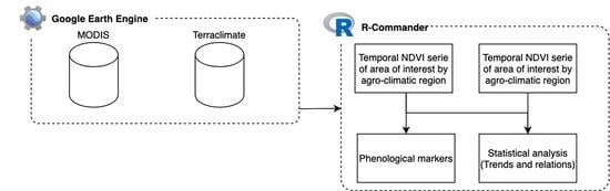
2.3. Datasets and Image Processing

Figure 4 summarizes the methodology applied to this research. MODIS MOD13Q1 normalized difference vegetation index (NDVI) [57] was used as the remote sensing dataset, while TERRACLIMATE [58] was used as the climate database. The extraction of remote sensing and climate data for the study area between 2001 and 2020 was carried out with Google Earth Engine (GEE) using Earth Engine Python API as the client server to connect with Earth Engine Services. These extracted data, stored in Google Drive, were downloaded for further processing on a local machine. Information on the areas occupied by grasslands as well as the delimitation of the agro-climatic regions was obtained from the Corporación Nacional Forestal (CONAF) [59]. Grassland areas for each region were used to determine accumulated rainfall, maximum and minimum temperature, and NDVI trends. These data were then analyzed to determine the statistical relationships between climatic variables and NDVI. The phenological markers of the grassland were determined according to each agro-climatic region.
MODIS MOD13Q1 [57] data were used to study spatiotemporal changes in the grasslands. This dataset was computed from atmospherically corrected surface reflectance scenes with a temporal resolution of 16 days and a spatial resolution of 250 m. These were masked for water, clouds, cloud-shadow and heavy aerosols. Monthly climate data of maximum and minimum temperatures as well as rainfall were extracted from the TERRACLIMATE database.
A total of 480 MOD13Q1 NDVI images, as well as 240 images for each climatic variable, maximum and minimum temperature, and rainfall, from TERRACLIMATE from 2001 to 2021 were extracted. In addition, as TERRACLIMATE data have a monthly resolution, MOD13Q1 NDVI data were processed using the Maximum Value Composites (MVC) method to acquire monthly NDVI. We used the MVC method to avoid the influence of solar altitude angle, clouds and/or atmospheric effects [60], thus permitting the study of the relationships between the two types of variables.

2.4. NDVI Time-Series

The phenological markers SOS, EOS, the peak of maximum NDVI and the grassland values from 2001 to 2020 were extracted from the MOD13Q1 dataset. Firstly, referencing land coverage and land use (LCLU) maps from CONAF [59], pure pixels occupied by grasslands were identified. In order to perform this, the polygons categorized as grasslands were extracted and intersected with the MODIS pixel grid. On this spatial division, only those pixels completely occupied by grassland were selected for each agro-climatic region, thereby removing mixed pixels. For each MOD13Q1 scene and agro-climatic region, the median NDVI was determined, obtaining six NDVI time-series, one for each agroclimatic region, with a temporal resolution of 16 days. R-commander was used for this purpose.
The six NDVI time-series were processed with TIMESAT software v3.3 [53] where annual NDVI values were smoothed using the Savitzky–Golay filter [61]. The phenological markers were determined as the 20% of the season amplitude from the left and right minimum values of NDVI fitted values, respectively [62,63]. Based on previous research [64], grassland phenology for each agro-climatic region was summarized as they are relatively homogeneous both in climate and biological diversity.

2.5. Statistical Analysis

First, to obtain an overview of the dynamics of the climate variables, the mean value of these variables for the period of 2001–2020 was determined for each month. Subsequently, for each month and year, their difference with the monthly mean value for the whole period was determined. These differences were represented by annual density plots to describe the behavior of the variables over the period analyzed.
Secondly, climatic variables and NDVI time series were decomposed into trend, cycle and residual. Trend corresponds to a long-term process that occurs over time, and the cycle explains the cyclical process that operates for each cycle once the trend is accounted for and residual, obtained after accounting for trend and cycle, explains local process caused by variability between cycles. Next, via cross-correlation analysis, the relationships between NDVI values and climatic variables for each agro-climatic region were examined in order to evaluate the climatic dependency of the Biobio grasslands.
Finally, as in other research [65,66], temporal trends in the data sets were evaluated with a linear regression model in which time was the independent variable while phenological markers were the dependent variables.

3. Results

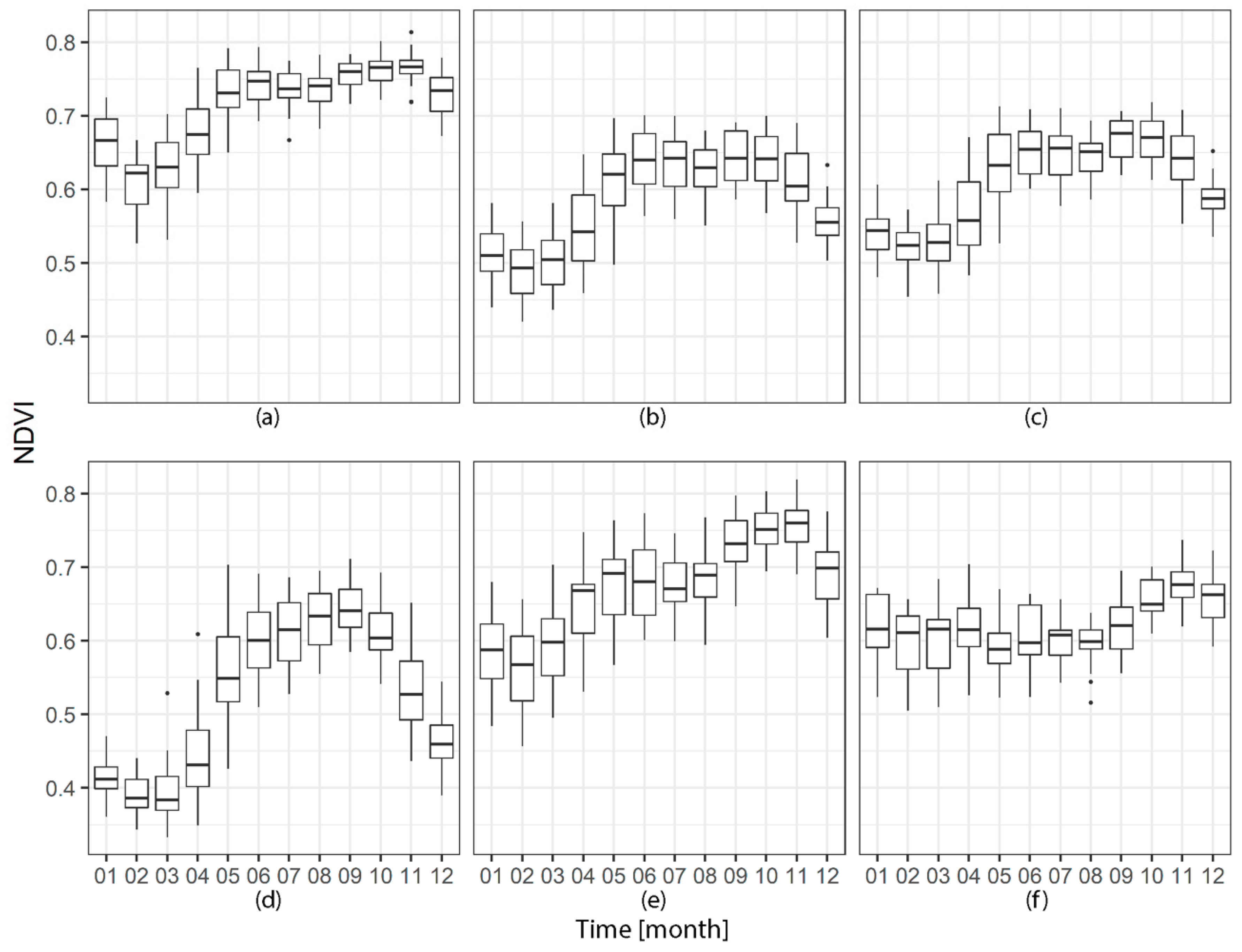
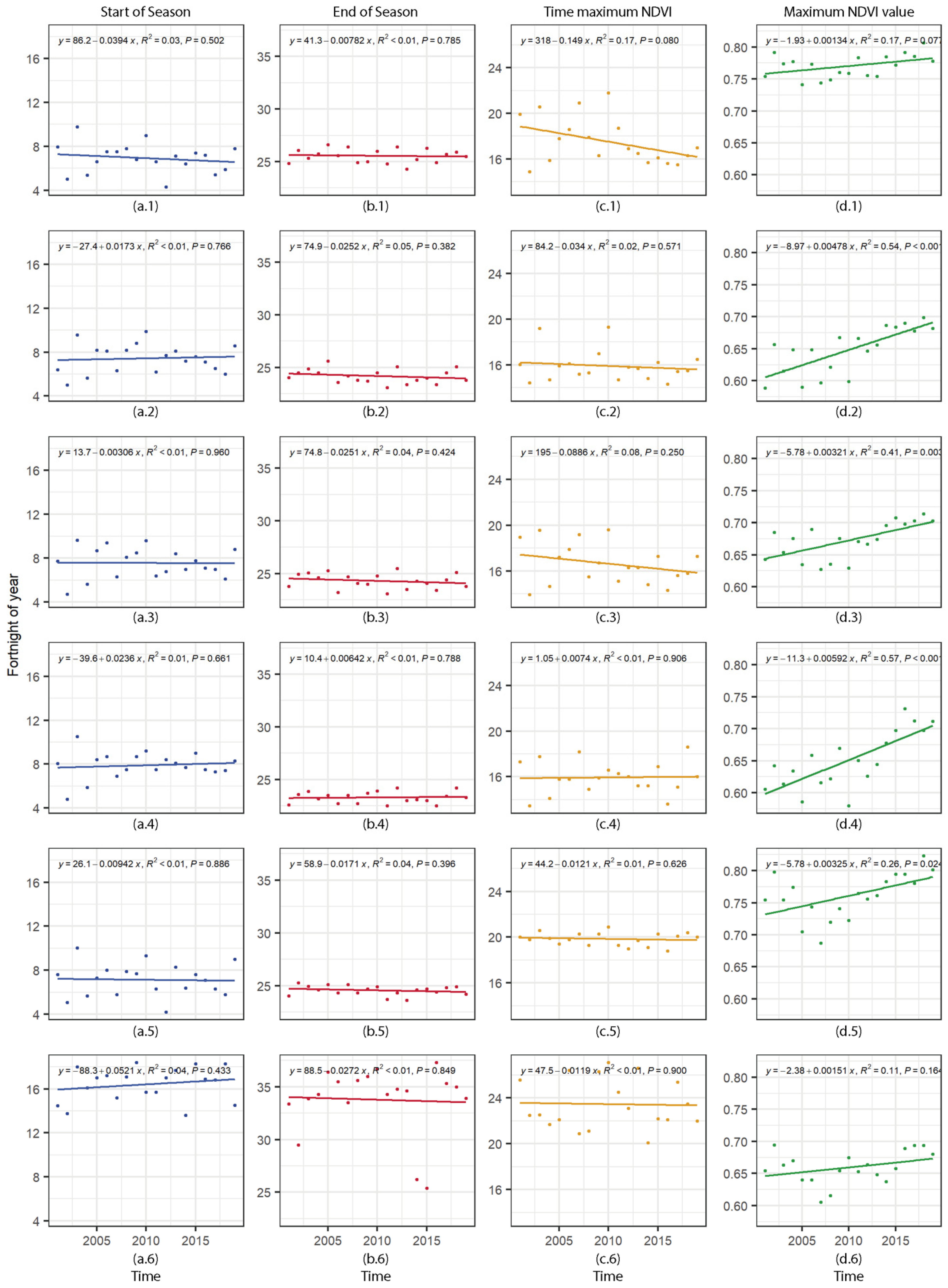
3.1. NDVI Time-Series

The evolution of the monthly mean NDVI for the six regions studied is shown in Figure 5. Each region shows a different development curve. Thus, in regions such as the Cordillera (Figure 5f), there is little variation in NDVI throughout the year, while in Cordón Isla (Figure 5d), there is a greater difference in the NDVI values recorded in the different seasons of the year. For the Secano Costero region (Figure 5a), the month with the lowest NDVI value was February (0.62), rising to stabilize in May, reaching the maximum value in November (0.76). In addition, the month with the highest interquartile range was January (0.06), and the lowest was November (0.01), both close to SOS and EOS. The regions of Secano Interior (Figure 5b), and Depresión Intermedia (Figure 5c) show a similar NDVI evolution. In the case of the Secano Interior region (Figure 5b), the minimum and maximum NDVI values appear in February (0.49) and July (0.64), respectively, with December and April showing the lowest and highest variability, the interquartile ranges being equal to 0.03 and 0.08. The Depression Intermedia region (Figure 5c) had the highest NDVI value in September (0.67) and the lowest in February (0.52), the months with the highest variability being the same as in Secano Interior.
Cordon Isla (Figure 5d) is the region with the greatest differences in NDVI between months. The lowest NDVI value is March (0.383), and the highest is September (0.641). From March to May, the NDVI increases progressively, the latter being the one with the largest interquartile range (0.08). Until September, the NDVI remains stable at high values and then starts to decrease. For the Precordillera region (Figure 5e), the NDVI has its lowest values in February (0.56). From February onwards, the index increases progressively until November (0.76), where it starts to decrease. Finally, the Cordillera region (Figure 5f) is the one with the most stable NDVI value annually, with respective maximum and minimum values of 0.67 in November and 0.58 in May, registering the highest interquartile range in the season of growth for grasslands (December–March).
Seasonal parameters, SOS and EOS, extracted from TIMESAT for each agro-climatic region are shown in Table 1, where the term season refers to the annual cycle of NDVI. In addition, Figure A4 in Appendix A represents the NDVI time series and phenological markers SOS and EOS for each agro-climatic region. Based on these data, in the Biobío region, the average SOS between 2001 and 2020 is on the day of the year (DOY) 133, while EOS is on 388, resulting in a mean duration of the grassland cycle equal to 255. However, each agro-climatic region presented different phenological markers. The grasslands in the Secano Costero region are the ones that start the cycle earlier (SOS equals DOY 103). As they move away from the coast towards the interior, SOS increases until reaching the Precordillera region, where SOS decreases. Thus, mean SOS in Secano Interior, Depresión Intermedia, Cordón Isla and Precordillera appears on DOY 111, 113, 118 and 107, respectively. Finally, the grasslands in the Cordillera region present the greatest delayed mean SOS with a DOY equal to 245. On the other hand, EOS markers in grasslands according to the agro-climatic region do not show a pattern similar to SOS. The Cordillera region presents a mean EOS in DOY 506, i.e., the grassland cycle is between two years, while Cordon Isla presents in DOY 349. On the other hand, Secano Costero, Secano Interior, Depresión Intermedia and Precordillera present a mean SOS in DOYs equal to 383, 361, 364, 349 and 368, respectively. With these phenological markers, the average grassland cycle in the Biobio regions ranges from 279 days in Secano Costero to 231 days in Cordon Isla. In the Secano Interior and Depresión Intermedia regions, the average grassland cycle is 250 days, while in the Precordillera and Cordillera, it is 260 days.

3.2. Analysis of Relations between Climatic Variables and NDVI

Previous research projects have shown that the time lag between NDVI to climatic factors ranges from 0 to 3 months [67,68,69]. Each agro-climatic region was analyzed for the correlation coefficient values between concurrent average monthly NDVI and concurrent average monthly climatic variables (lag 0), the monthly average of the previous month (lag 1) and monthly averages of the two previous months (lag 2) (Table 2).
Positive correlation results between accumulated rainfall and NDVI were obtained in lag 0 and 1 for all agro-climatic regions, while for lag 2, the Cordillera region showed a negative correlation, mainly due to the presence of snow. Accumulated rainfall and NDVI showed a significant positive correlation from lag 0 and, therefore, an immediate positive impact on grasslands. Particularly, in Secano Costero, Precordillera and Cordillera, the response of NDVI to accumulated rainfall showed the highest correlation at lag 0 while in Secano Interior, Depresión Intermedia and Cordón Isla was at lag 1, which means that the highest positive effect appears the following month. In Lag 2, high values are maintained above all in the areas where it rains less, Secano Interior, Depresión Intermedia and Cordón Isla. However, in the areas where rainfall is less necessary, a drop in the correlation in lag 2 can be observed. For maximum and minimum temperature, except in the Cordillera region, the highest correlations were obtained in Lag 0 for both maximum and minimum temperatures. The correlation was negative, indicating that higher temperatures have a negative effect on NDVI, reducing it. Moreover, its effect on grassland appears immediately, with lag equal to 0. The Cordon Isla region showed the highest values, corresponding to the driest region of all the analyzed regions. At the opposite extreme, temperatures in the Cordillera region, both maximum and minimum, have a positive effect on vegetation, increasing the NDVI. The result of an increase in temperature is reflected in the following two months (Lag 2). The results obtained show how climatic variables are related to NDVI values. Thus, an increase in rainfall results in an increase in NDVI values, while they decrease with increasing temperatures.
Having proved that climatic variables influence grassland development in Biobio, with a growing tendency towards reduced rainfall and increased maximum and minimum temperatures, the general trend and phenological markers of NDVI in each region between 2001 and 2020 are presented below. Trends of NDVI values for each region are shown in Figure 6. The trends of the NDVI series of the agro-climatic regions in Biobio show a similar pattern, differentiating an initial period with little change in the NDVI and a second period with an increase in the index. Thus, between 2001 and 2007, NDVI values do not show a clear change in their evolution. In 2008 there was a reduction in the NDVI value in each region, and from that year onwards, there was an increase in NDVI, with greater or lesser intensity depending on the agro-climatic region. Such NDVI trends are aligned with the evolution of the climatic variables presented in Section 3.1. Of all the regions, the Secano Costero region is the one with the highest NDVI values and the smallest increase, presenting stability compared to the other regions. On the other hand, the Precordillera region presents the highest increase in NDVI, reaching similar values to the Secano Costero region in recent years. The Secano Interior and Depresión Intermedia regions behave similarly, with shared increases in NDVI, but more moderately than in the Precordillera region. The Cordillera region has NDVI values in the same range as the two previous regions, although with more accentuated fluctuations over time.
Figure 7 represents the trends of phenological markers: SOS (Figure 7a), EOS (Figure 7b), the peak of the season (Figure 7c) and NDVI (Figure 7d) over time during the 2001–2020 period. In general, the trend changes in grassland phenology at the peak of maximum NDVI and its value in the period 2001–2020 are more pronounced than SOS and EOS. In the Secano Costero region, the temporal relationships between SOS (Figure 7(a.1)) and EOS (Figure 7(b.1)) slope negatively, which means both growth periods occur earlier, although the duration of the cycle stays the same. This same behavior appears in the Depresión Intermedia (Figure 7(a.3,b.3) and Precordillera (Figure 7(a.5,b.5)) regions. On the other hand, the Secano Interior and Cordillera region present with positive slopes in SOS (Figure 7(a.2,a.6)) and a negative slope in EOS (Figure 7(b.2,b.6)). This means a reduction in the phenological cycle of the grasslands in these regions due to the delay of SOS and the advancement of EOS. Finally, the Cordon Isla region has a positive slope in both SOS (Figure 7(a.4)) and EOS (Figure 7(b.4)) so that there is a delay in the entire grassland cycle in this region without major changes in the duration of the cycle. Based on the low values obtained in the slopes of the SOS and EOS trends, there appear to be no important changes in the start or end of the phenological cycle of the grasslands.
When analyzing the results obtained in the trend at the moment of reaching the maximum NDVI (Figure 7c), as well as its value (Figure 7d), there is a general trend to reach maximum NDVI earlier (negative slope) and with a higher value in the index (positive slope). It is in the regions of Secano Costero (Figure 7(c.1)) and Depresión Intermedia (Figure 7(c.3)) where there is a more evident advance in reaching maximum vigor, with a higher negative slope. Secano Interior (Figure 7(c.2)), Precordillera (Figure 7(c.5)) and Cordillera (Figure 7(c.6)) show this advance as well but in a less accentuated manner. Cordón Isla (Figure 7(c.4)) is the only region that shows a delay in this marker. Finally, all regions show an upward trend in NDVI, with Cordon Isla (Figure 7(d.4)) showing the greatest increment over time, while the Secano Costero (Figure 7(d.1)) and Cordillera (Figure 7(d.6)) regions show the smallest.

4. Discussion

Phenological observations provide localized information with high temporal resolutions in different biological phases. Phenology varies over geographic gradients according to climate zone and vegetation type. Phenology also varies within communities, and the phenology of individual plants plays a key role in determining how ecosystems are structured and how they function [70]. Temperate forest trends are attributed to warming temperatures [23,71]. In addition, boreal and subalpine forests show similar trends to those observed in temperate forests, which are attributed to a warming climate [72,73]; moreover, there is little evidence that rainfall has a significant influence on boreal forest phenology [74]. In Subalpine meadows and the Arctic and alpine tundras, in high latitudes and high altitude ecosystems, there are two main factors that regulate SOS, the timing of snowmelt and the temperatures that follow [75] while warm might delay EOS [76]; however, it has not been extensively studied. On the other hand, the impacts of climate change on tropical forests vary across regional-to-continental scales. Decreasing precipitation and reduced cloudiness in Amazonia may result in different phenological shifts than, for example, in central Africa, where precipitation is projected to increase [77]. Mediterranean areas include a diverse range of plant types, and phenological responses to environmental cues vary accordingly. Temperature is a key factor for most species, but rainfall, through its influence on soil moisture, is also important [78,79]. Finally, in subtropical desert ecosystems, phenological variations resulting from climate change may occur due to changes in the timing and quantity of rainfall and increases in temperature [80]. Therefore, phenology varies over geographic gradients according to climate zone and vegetation type.
In contrast to direct phenological observations, satellite data have the advantage of high spatial coverage. It allows global, regional, and local studies. NDVI and climatic time series provide key information in the study of vegetation. The analysis of vegetation requires a spatial and temporal approach to explain changes and dynamics in vegetation. Temporal, seasonal and phenological metrics obtained by vegetation index series from remote sensing scenes provide useful information to understand vegetation conditions at regional scales. Taking into account previous research, the climatic response of grasslands varies geographically. Previous studies have shown that a warming climate has a positive impact on greening in the northern hemisphere, relying on the continuously warming air and spatially uneven trends of precipitation [81,82]. However, increased temperatures could not be the primary control of grassland. Rainfall is a factor that plays a relevant role in grassland. In the Biobio region, temperature increase from 2001 to 2020 has extended the period where conditions are favorable to plant growth; however, the grasslands have not benefitted from these conditions. Instead, grasslands in Biobio have shown little change at SOS and EOS. However, photosynthetic capacity, measured by NDVI, has increased significantly in all the agro-climatic regions of Biobio. These trends show how grasslands grow faster and more vigorously as temperatures increase. On the other hand, the incapacity of grasslands to exploit thermal resources can be potentially explained by a mismatch between current vegetation and climate conditions, which could be explained by the novel conditions caused by climate change, such as the reduction in rainfall. These results presented here align with other research, such as those in the Tibetan Plateau [83].
Grasslands are very sensitive to rainfall, so more arid conditions would lead to lower productivity. However, a decrease in winter frosts through higher minimum temperatures, higher temperatures in general and higher solar radiation would compensate for the negative effect of lower rainfall and may even result in a slight increase in productivity [84]. This contradictory situation could also be explained by the beneficial effect of high CO2 concentrations in the atmosphere, which stimulates net plant photosynthesis [85], improving their growth and productivity [86,87], and water use efficiency [88]. CO2 concentration can be measured through the use of onboard sensors on satellite platforms such as Sentinel 5P, GOSAT or OCO-2. These platforms have only recently been launched, however, and there are not enough data to create robust time-series data to analyze; thus, future work should evaluate climate and atmospheric variables together.
Therefore, recent warming trends have been associated with earlier vegetation activity in spring and an overall extension in the length of the growing season [89]. On the other hand, there is less of a consensus on how climate change is affecting end-of-season phenology, although many biological events are observed to be occurring later [90].
While no comparisons have been made in this study between ground observations and the remote sensing-based results, this type of activity is needed to more fully understand and validate remote sensing-based observations of large-scale phenology in terrestrial vegetation.
On the other hand, variations in climate conditions have an important impact on water balance and material circulation in watersheds. Thus, the influence of climate change on water quality has been previously documented [91,92]. It is assumed that climate change can influence water environments by affecting water flow, pollutant transformation and migration, as well as toxicity [93,94]. Moreover, transformation and migration patterns of toxic pollutants in the water environment are complex processes, and the influencing mechanism of climate change on heavy metals is still unknown. Recently, a few studies demonstrated the impact of meteorological factors on heavy metals using model simulation methods or short-term water quality data [95,96]. High heavy metal concentrations in soils were cited as one of the factors limiting vegetation establishment and growth in areas suffering high anthropogenic impact [97,98,99]. Thus, heavy metal toxicity first affects the growth of vegetation roots because they are more sensitive to heavy metal stress. In addition, heavy metal pollution limits root growth and results in decreased root weight [100,101]. Based on previous research in the study area [102,103,104,105], future projects should analyze the influence of heavy metal and contaminant concentrations in soil, together with climatic variables and vegetation indices, to study changes in the phenology of vegetation, including grasslands.
Based on article 4.8 of the United Nations Framework Convention on Climate Change [106], Chile meets 7 of the 9 vulnerability characteristics to be identified as a region in the world affected by the alteration of the current global climate pattern. The map of grassland phenology in the Biobio region can support decision-making in monitoring vulnerability to climate variations and therefore serves as a useful tool for assessing measures taken against climate change.

5. Conclusions

In a scenario where climatic conditions are changing, monitoring tools are required to understand impacts on vegetation better. Therefore, an understanding of the drivers involved in phenology is needed even when detailed field observations are lacking, and meteorological stations are scarce. This result makes remote sensing datasets for vegetation monitoring a particularly useful tool under these scenarios. In this study, we evaluated the timing of phenology markers and their response to climate conditions in six agro-climatic regions in Biobio. Our results suggest that climatic conditions in Biobio have become more conducive to grassland growth over the 2001–2020 period. During this period, rainfall has decreased; however, favorable thermal conditions have extended. In this context, the grasslands have shown more intensive photosynthetic activity but without extending the period of activity. The six areas analyzed show that between 2001 and 2010, the evolution of NDVI values was stable. However, between 2010 and 2020, there was an increase in NDVI values to a greater or lesser extent depending on the area analyzed. The Precordillera region shows the greatest increase, while Secano Costero is the most stable.
In general, the results from this study highlight the relationship between grassland phenology and their response to the climatic variables of accumulated rainfall and temperature, both maximum and minimum, which has implications for developing policy frameworks for grassland management and protection and its relationship with future climate change.

Author Contributions

Conceptualization, M.-A.D.-G., F.-J.P.-P. and F.-J.M.-C.; methodology, M.-A.D.-G., F.-J.P.-P. and F.-J.M.-C.; validation, P.T.-T.; A.-F.R.-M. and A.G.-F.P.; formal analysis, M.-A.D.-G. and F.-J.M.-C.; writing—original draft preparation, F.-J.M.-C.; writing—review and editing, M.-A.D.-G., F.-J.P.-P. and F.-J.M.-C. All authors have read and agreed to the published version of the manuscript.

Funding

This research received no external funding.

Institutional Review Board Statement

Not applicable.

Informed Consent Statement

Not applicable.

Data Availability Statement

Not applicable.

Conflicts of Interest

The authors declare no conflict of interest.

Appendix A

Figure A1. Box-plot of accumulated rainfall per month for the agro-climatics areas of Biobio: (a) Secano Costero, (b) Secano interior, (c) Depresión Intermedia, (d) Cordón Isla, (e) Precordillera and (f) Cordillera.
Remotesensing 14 00475 g0a1
Figure A2. Box-plot of maximum temperature per month for the agro-climatics areas of Biobio: (a) Secano Costero, (b) Secano interior, (c) Depresión Intermedia, (d) Cordón Isla, (e) Precordillera and (f) Cordillera.
Remotesensing 14 00475 g0a2
Figure A3. Box-plot of minimum temperature per month for the agro-climatics areas of Biobio: (a) Secano Costero, (b) Secano interior, (c) Depresión Intermedia, (d) Cordón Isla, (e) Precordillera and (f) Cordillera.
Remotesensing 14 00475 g0a3
Figure A4. NDVI seasonal analysis with raw MODIS and fitted data marked as start of season and end of season from 2001 to 2020 in the six agro-climatics regions of Biobio: (a) Secano Costero, (b) Secano Interior, (c) Depresión Intermedia, (d) Cordón Isla, (e) Precordillera and (f) Cordillera.
Remotesensing 14 00475 g0a4

References

  1. Myneni, R.B.; Keeling, C.D.; Tucker, C.J.; Asrar, G.; Nemani, R.R. Increased plant growth in the northern high latitudes from 1981 to 1991. Nature 1997, 386, 698–702. [Google Scholar] [CrossRef]
  2. Piao, S.; Liu, Q.; Chen, A.; Janssens, I.A.; Fu, Y.; Dai, J.; Liu, L.; Lian, X.; Shen, M.; Zhu, X. Plant phenology and global climate change: Current progresses and challenges. Glob. Chang. Biol. 2019, 25, 1922–1940. [Google Scholar] [CrossRef] [PubMed]
  3. Justice, C.O.; Holben, B.N.; Gwynne, M.D. Monitoring East African vegetation using AVHRR data. Int. J. Remote Sens. 1986, 7, 1453–1474. [Google Scholar] [CrossRef]
  4. McCloy, K.R. Development and Evaluation of Phenological Change Indices Derived from Time Series of Image Data. Remote Sens. 2010, 2, 2442–2473. [Google Scholar] [CrossRef] [Green Version]
  5. Peñuelas, J.; Filella, I.; Zhang, X.; Llorens, L.; Ogaya, R.; Lloret, F.; Comas, P.; Estiarte, M.; Terradas, J. Complex spatiotemporal phenological shifts as a response to rainfall changes. New Phytol. 2004, 161, 837–846. [Google Scholar] [CrossRef]
  6. Conant, R.T. Challenges and Opportunities for Carbon Sequestration in Grassland Systems; A Technical Report on Grassland Management and Climate Change Mitigation; Food and Agriculture Organization of the United Nations: Rome, Italy, 2010. [Google Scholar]
  7. Lal, R. Soil Carbon Sequestration Impacts on Global Climate Change and Food Security. Science 2004, 304, 1623–1627. [Google Scholar] [CrossRef] [Green Version]
  8. Hall, D.O.; Scurlock, J.M.O.; Ojima, D.S.; Parton, W.J. Grasslands and the Global Carbon Cycle: Modeling the Effects of Climate Change. In The Carbon Cycle; Wigley, T.M.L., Schimel, D.S., Eds.; Cambridge University Press: Cambridge, UK, 2000; pp. 102–114. [Google Scholar]
  9. O’Mara, F.P. The role of grasslands in food security and climate change. Ann. Bot. 2012, 110, 1263–1270. [Google Scholar] [CrossRef] [Green Version]
  10. Bloor, J.M.G.; Pichon, P.; Falcimagne, R.; Leadley, P.W.; Soussana, J.-F. Effects of Warming, Summer Drought, and CO2 Enrichment on Aboveground Biomass Production, Flowering Phenology, and Community Structure in an Upland Grassland Ecosystem. Ecosystems 2010, 13, 888–900. [Google Scholar] [CrossRef]
  11. Piao, S.; Fang, J.; Zhou, L.; Ciais, P.; Zhu, B. Variations in satellite-derived phenology in China’s temperate vegetation. Glob. Chang. Biol. 2006, 12, 672–685. [Google Scholar] [CrossRef]
  12. Xia, J.; Wan, S. Independent effects of warming and nitrogen addition on plant phenology in the Inner Mongolian steppe. Ann. Bot. 2013, 111, 1207–1217. [Google Scholar] [CrossRef] [PubMed]
  13. Wu, X.; Liu, H. Consistent shifts in spring vegetation green-up date across temperate biomes in China, 1982–2006. Glob. Chang. Biol. 2013, 19, 870–880. [Google Scholar] [CrossRef] [PubMed]
  14. Hovenden, M.J.; Wills, K.E.; Schoor, J.K.V.; Williams, A.L.; Newton, P.C.D. Flowering phenology in a species-rich temperate grassland is sensitive to warming but not elevated CO2. New Phytol. 2008, 178, 815–822. [Google Scholar] [CrossRef] [Green Version]
  15. Vrieling, A.; de Leeuw, J.; Said, M.Y. Length of Growing Period over Africa: Variability and Trends from 30 Years of NDVI Time Series. Remote Sens. 2013, 5, 982–1000. [Google Scholar] [CrossRef] [Green Version]
  16. Fu, Y.H.; Piao, S.; de Beeck, M.O.; Cong, N.; Zhao, H.; Zhang, Y.; Menzel, A.; Janssens, I.A. Recent spring phenology shifts in western Central Europe based on multiscale observations. Glob. Ecol. Biogeogr. 2014, 23, 1255–1263. [Google Scholar] [CrossRef]
  17. Zhang, G.; Zhang, Y.; Dong, J.; Xiao, X. Green-up dates in the Tibetan Plateau have continuously advanced from 1982 to 2011. Proc. Natl. Acad. Sci. USA 2013, 110, 4309–4314. [Google Scholar] [CrossRef] [PubMed] [Green Version]
  18. Zhang, X.; Friedl, M.A.; Schaaf, C.B.; Strahler, A.H.; Liu, Z. Monitoring the response of vegetation phenology to precipitation in Africa by coupling MODIS and TRMM instruments. J. Geophys. Res. Atmos. 2005, 110. Available online: https://agupubs.onlinelibrary.wiley.com/doi/full/10.1029/2004JD005263 (accessed on 11 December 2021). [CrossRef]
  19. Fu, Y.H.; Zhao, H.; Piao, S.; Peaucelle, M.; Peng, S.; Zhou, G.; Ciais, P.; Huang, M.; Menzel, A.; Peñuelas, J.; et al. Declining global warming effects on the phenology of spring leaf unfolding. Nature 2015, 526, 104–107. [Google Scholar] [CrossRef] [Green Version]
  20. Shen, M.; Tang, Y.; Chen, J.; Yang, X.; Wang, C.; Cui, X.; Yang, Y.; Han, L.; Li, L.; Du, J.; et al. Earlier-Season Vegetation Has Greater Temperature Sensitivity of Spring Phenology in Northern Hemisphere. PLoS ONE 2014, 9, e88178. [Google Scholar] [CrossRef] [PubMed]
  21. Forkel, M.; Migliavacca, M.; Thonicke, K.; Reichstein, M.; Schaphoff, S.; Weber, U.; Carvalhais, N. Codominant water control on global interannual variability and trends in land surface phenology and greenness. Glob. Chang. Biol. 2015, 21, 3414–3435. [Google Scholar] [CrossRef] [PubMed]
  22. Workie, T.G.; Debella, H.J. Climate change and its effects on vegetation phenology across ecoregions of Ethiopia. Glob. Ecol. Conserv. 2018, 13, 00366. [Google Scholar] [CrossRef]
  23. Jeong, S.-J.; Ho, C.-H.; Gim, H.-J.; Brown, M.E. Phenology shifts at start vs. end of growing season in temperate vegetation over the Northern Hemisphere for the period 1982–2008. Glob. Chang. Biol. 2011, 17, 2385–2399. [Google Scholar] [CrossRef]
  24. Chmielewski, F.-M.; Müller, A.; Bruns, E. Climate changes and trends in phenology of fruit trees and field crops in Germany, 1961–2000. Agric. For. Meteorol. 2004, 121, 69–78. [Google Scholar] [CrossRef]
  25. Crimmins, T.M.; Crimmins, M.A.; Bertelsen, C.D. Complex responses to climate drivers in onset of spring flowering across a semi-arid elevation gradient. J. Ecol. 2010, 98, 1042–1051. [Google Scholar] [CrossRef]
  26. Dash, J.; Jeganathan, C.; Atkinson, P.M. The use of MERIS Terrestrial Chlorophyll Index to study spatio-temporal variation in vegetation phenology over India. Remote Sens. Environ. 2010, 114, 1388–1402. [Google Scholar] [CrossRef]
  27. Zhang, X.; Friedl, M.A.; Schaaf, C.B.; Strahler, A.H.; Hodges, J.C.F.; Gao, F.; Reed, B.C.; Huete, A. Monitoring vegetation phenology using MODIS. Remote Sens. Environ. 2003, 84, 471–475. [Google Scholar] [CrossRef]
  28. Jin, C.; Xiao, X.; Merbold, L.; Arneth, A.; Veenendaal, E.; Kutsch, W.L. Phenology and gross primary production of two dominant savanna woodland ecosystems in Southern Africa. Remote Sens. Environ. 2013, 135, 189–201. [Google Scholar] [CrossRef]
  29. Hufkens, K.; Friedl, M.; Sonnentag, O.; Braswell, B.H.; Milliman, T.; Richardson, A.D. Linking near-surface and satellite remote sensing measurements of deciduous broadleaf forest phenology. Remote Sens. Environ. 2012, 117, 307–321. [Google Scholar] [CrossRef]
  30. Zhu, W.; Tian, H.; Xu, X.; Pan, Y.; Chen, G.; Lin, W. Extension of the growing season due to delayed autumn over mid and high latitudes in North America during 1982–2006. Glob. Ecol. Biogeogr. 2012, 21, 260–271. [Google Scholar] [CrossRef]
  31. White, M.A.; de Beurs, K.M.; Didan, K.; Inouye, D.W.; Richardson, A.D.; Jensen, O.P.; O’Keefe, J.; Zhang, G.; Nemani, R.R.; van Leeuwen, W.J.D.; et al. Intercomparison, interpretation, and assessment of spring phenology in North America estimated from remote sensing for 1982–2006. Glob. Chang. Biol. 2009, 15, 2335–2359. [Google Scholar] [CrossRef]
  32. Xie, Y.; Sha, Z.; Yu, M. Remote sensing imagery in vegetation mapping: A review. J. Plant Ecol. 2008, 1, 9–23. [Google Scholar] [CrossRef]
  33. de Beurs, K.M.; Henebry, G.M. Land surface phenology and temperature variation in the International Geosphere-Biosphere Program high-latitude transects. Glob. Chang. Biol. 2005, 11, 779–790. [Google Scholar] [CrossRef]
  34. Wu, C.; Peng, D.; Soudani, K.; Siebicke, L.; Gough, C.M.; Arain, M.A.; Bohrer, G.; Lafleur, P.M.; Peichl, M.; Gonsamo, A.; et al. Land surface phenology derived from normalized difference vegetation index (NDVI) at global FLUXNET sites. Agric. For. Meteorol. 2017, 233, 171–182. [Google Scholar] [CrossRef]
  35. Hou, X.; Gao, S.; Niu, Z.; Xu, Z. Extracting grassland vegetation phenology in North China based on cumulative SPOT-VEGETATION NDVI data. Int. J. Remote Sens. 2014, 35, 3316–3330. [Google Scholar] [CrossRef]
  36. Wang, C.; Li, J.; Liu, Q.; Zhong, B.; Wu, S.; Xia, C. Analysis of Differences in Phenology Extracted from the Enhanced Vegetation Index and the Leaf Area Index. Sensors 2017, 17, 1982. [Google Scholar] [CrossRef] [Green Version]
  37. Cao, R.; Chen, J.; Shen, M.; Tang, Y. An improved logistic method for detecting spring vegetation phenology in grasslands from MODIS EVI time-series data. Agric. For. Meteorol. 2015, 200, 9–20. [Google Scholar] [CrossRef]
  38. Ahl, D.E.; Gower, S.T.; Burrows, S.N.; Shabanov, N.V.; Myneni, R.B.; Knyazikhin, Y. Monitoring spring canopy phenology of a deciduous broadleaf forest using MODIS. Remote Sens. Environ. 2006, 104, 88–95. [Google Scholar] [CrossRef] [Green Version]
  39. Testa, S.; Soudani, K.; Boschetti, L.; Mondino, E.B. MODIS-derived EVI, NDVI and WDRVI time series to estimate phenological metrics in French deciduous forests. Int. J. Appl. Earth Obs. Geoinf. 2018, 64, 132–144. [Google Scholar] [CrossRef]
  40. Li, X.; Du, H.; Zhou, G.; Mao, F.; Zhang, M.; Han, N.; Fan, W.; Liu, H.; Huang, Z.; He, S.; et al. Phenology estimation of subtropical bamboo forests based on assimilated MODIS LAI time series data. ISPRS J. Photogramm. Remote Sens. 2021, 173, 262–277. [Google Scholar] [CrossRef]
  41. Moon, M.; Seyednasrollah, B.; Richardson, A.D.; Friedl, M.A. Using time series of MODIS land surface phenology to model temperature and photoperiod controls on spring greenup in North American deciduous forests. Remote Sens. Environ. 2021, 260, 112466. [Google Scholar] [CrossRef]
  42. Yang, Y.; Ren, W.; Tao, B.; Ji, L.; Liang, L.; Ruane, A.C.; Fisher, J.B.; Liu, J.; Sama, M.; Li, Z.; et al. Characterizing spatiotemporal patterns of crop phenology across North America during 2000–2016 using satellite imagery and agricultural survey data. ISPRS J. Photogramm. Remote Sens. 2020, 170, 156–173. [Google Scholar] [CrossRef]
  43. Choudhary, K.; Shi, W.; Boori, M.S.; Corgne, S. Agriculture Phenology Monitoring Using NDVI Time Series Based on Remote Sensing Satellites: A Case Study of Guangdong, China. Opt. Mem. Neural Netw. 2019, 28, 204–214. [Google Scholar] [CrossRef]
  44. Liang, L.; Zhao, S.-H.; Qin, Z.-H.; He, K.-X.; Chen, C.; Luo, Y.-X.; Zhou, X.-D. Drought Change Trend Using MODIS TVDI and Its Relationship with Climate Factors in China from 2001 to 2010. J. Integr. Agric. 2014, 13, 1501–1508. [Google Scholar] [CrossRef]
  45. Klisch, A.; Atzberger, C. Operational Drought Monitoring in Kenya Using MODIS NDVI Time Series. Remote Sens. 2016, 8, 267. [Google Scholar] [CrossRef] [Green Version]
  46. Li, R.; Xu, M.; Chen, Z.; Gao, B.; Cai, J.; Shen, F.; He, X.; Zhuang, Y.; Chen, D. Phenology-based classification of crop species and rotation types using fused MODIS and Landsat data: The comparison of a random-forest-based model and a decision-rule-based model. Soil Tillage Res. 2021, 206, 104838. [Google Scholar] [CrossRef]
  47. Liu, Q.; Piao, S.; Janssens, I.A.; Fu, Y.; Peng, S.; Lian, X.; Ciais, P.; Myneni, R.B.; Peñuelas, J.; Wang, T. Extension of the growing season increases vegetation exposure to frost. Nat. Commun. 2018, 9, 426. [Google Scholar] [CrossRef] [Green Version]
  48. Zheng, Y.; Wu, B.; Zhang, M.; Zeng, H. Crop Phenology Detection Using High Spatio-Temporal Resolution Data Fused from SPOT5 and MODIS Products. Sensors 2016, 16, 2099. [Google Scholar] [CrossRef] [PubMed] [Green Version]
  49. Atkinson, P.M.; Jeganathan, C.; Dash, J.; Atzberger, C. Inter-comparison of four models for smoothing satellite sensor time-series data to estimate vegetation phenology. Remote Sens. Environ. 2012, 123, 400–417. [Google Scholar] [CrossRef]
  50. Julien, Y.; Sobrino, J.A. Comparison of cloud-reconstruction methods for time series of composite NDVI data. Remote Sens. Environ. 2010, 114, 618–625. [Google Scholar] [CrossRef]
  51. Jin, Z.; Xu, B. A Novel Compound Smoother—RMMEH to Reconstruct MODIS NDVI Time Series. IEEE Geosci. Remote Sens. Lett. 2013, 10, 942–946. [Google Scholar] [CrossRef]
  52. Elmore, A.J.; Guinn, S.M.; Minsley, B.J.; Richardson, A.D. Landscape controls on the timing of spring, autumn, and growing season length in mid-Atlantic forests. Glob. Chang. Biol. 2012, 18, 656–674. [Google Scholar] [CrossRef] [Green Version]
  53. Jönsson, P.; Cai, Z.; Melaas, E.; Friedl, M.A.; Eklundh, L. A Method for Robust Estimation of Vegetation Seasonality from Landsat and Sentinel-2 Time Series Data. Remote Sens. 2018, 10, 635. [Google Scholar] [CrossRef] [Green Version]
  54. Zhang, G.P.; Qi, M. Neural network forecasting for seasonal and trend time series. Eur. J. Oper. Res. 2005, 160, 501–514. [Google Scholar] [CrossRef]
  55. Hijmans, R.J.; Cameron, S.E.; Parra, J.L.; Jones, P.G.; Jarvis, A. Very high resolution interpolated climate surfaces for global land areas. Int. J. Climatol. 2005, 25, 1965–1978. [Google Scholar] [CrossRef]
  56. Dietl, W.; Fernandez, F.; Venegas, C. Manejo Sostenible de Praderas: Su Flora y Vegetación; Instituto de Investigaciones Agropecuarias: Santiago de Chile, Chile, 2009. [Google Scholar]
  57. Didan, K. MOD13Q1 MODIS/Terra Vegetation Indices 16-Day L3 Global 250 m SIN Grid V006; Technical Report; NASA EOSDIS Land Processes DAAC: Sioux Falls, SD, USA, 2018.
  58. Abatzoglou, J.T.; Dobrowski, S.Z.; Parks, S.A.; Hegewisch, K.C. TerraClimate, a high-resolution global dataset of monthly climate and climatic water balance from 1958–2015. Sci. Data 2018, 5, 170191. [Google Scholar] [CrossRef] [Green Version]
  59. Corporación Nacional Forestal Sistema de Información Territorial CONAF. Available online: http://sit.conaf.cl/ (accessed on 7 December 2021).
  60. Gu, Z.; Duan, X.; Shi, Y.; Li, Y.; Pan, X. Spatiotemporal variation in vegetation coverage and its response to climatic factors in the Red River Basin, China. Ecol. Indic. 2018, 93, 54–64. [Google Scholar] [CrossRef]
  61. Chen, J.; Jönsson, P.; Tamura, M.; Gu, Z.; Matsushita, B.; Eklundh, L. A simple method for reconstructing a high-quality NDVI time-series data set based on the Savitzky–Golay filter. Remote Sens. Environ. 2004, 91, 332–344. [Google Scholar] [CrossRef]
  62. Cong, N.; Piao, S.; Chen, A.; Wang, X.; Lin, X.; Chen, S.; Han, S.; Zhou, G.; Zhang, X. Spring vegetation green-up date in China inferred from SPOT NDVI data: A multiple model analysis. Agric. For. Meteorol. 2012, 165, 104–113. [Google Scholar] [CrossRef]
  63. Zhou, D.; Zhao, S.; Zhang, L.; Liu, S. Remotely sensed assessment of urbanization effects on vegetation phenology in China’s 32 major cities. Remote Sens. Environ. 2016, 176, 272–281. [Google Scholar] [CrossRef] [Green Version]
  64. Riley, J.L.; Green, S.E.; Brodribb, K.E. A Conservation Blueprint for Canada’s Prairies and Parklands; Nature Conservancy of Canada: Toronto, ON, Canada, 2007; ISBN 1897386133. [Google Scholar]
  65. Tian, F.; Fensholt, R.; Verbesselt, J.; Grogan, K.; Horion, S.; Wang, Y.J. Evaluating temporal consistency of long-term global NDVI datasets for trend analysis. Remote Sens. Environ. 2015, 163, 326–340. [Google Scholar] [CrossRef]
  66. Fensholt, R.; Rasmussen, K.; Nielsen, T.T.; Mbow, C. Evaluation of earth observation based long term vegetation trends—Intercomparing NDVI time series trend analysis consistency of Sahel from AVHRR GIMMS, Terra MODIS and SPOT VGT data. Remote Sens. Environ. 2009, 113, 1886–1898. [Google Scholar] [CrossRef]
  67. Anderson, L.O.; Malhi, Y.; Aragão, L.E.O.C.; Ladle, R.; Arai, E.; Barbier, N.; Phillips, O. Remote sensing detection of droughts in Amazonian forest canopies. New Phytol. 2010, 187, 733–750. [Google Scholar] [CrossRef] [PubMed]
  68. Chen, T.; de Jeu, R.A.M.; Liu, Y.Y.; van der Werf, G.R.; Dolman, A.J. Using satellite based soil moisture to quantify the water driven variability in NDVI: A case study over mainland Australia. Remote Sens. Environ. 2014, 140, 330–338. [Google Scholar] [CrossRef]
  69. Zoungrana, B.J.-B.; Conrad, C.; Amekudzi, L.K.; Thiel, M.; Da, E.D. Land Use/Cover Response to Rainfall Variability: A Comparing Analysis between NDVI and EVI in the Southwest of Burkina Faso. Climate 2015, 3, 63–77. [Google Scholar] [CrossRef] [Green Version]
  70. Cleland, E.E.; Chuine, I.; Menzel, A.; Mooney, H.A.; Schwartz, M.D. Shifting plant phenology in response to global change. Trends Ecol. Evol. 2007, 22, 357–365. [Google Scholar] [CrossRef] [PubMed]
  71. Vitasse, Y.; Delzon, S.; Dufrêne, E.; Pontailler, J.-Y.; Louvet, J.-M.; Kremer, A.; Michalet, R. Leaf phenology sensitivity to temperature in European trees: Do within-species populations exhibit similar responses? Agric. For. Meteorol. 2009, 149, 735–744. [Google Scholar] [CrossRef]
  72. Pudas, E.; Leppälä, M.; Tolvanen, A.; Poikolainen, J.; Venäläinen, A.; Kubin, E. Trends in phenology of Betula pubescens across the boreal zone in Finland. Int. J. Biometeorol. 2008, 52, 251–259. [Google Scholar] [CrossRef]
  73. Nordli, Ø.; Wielgolaski, F.E.; Bakken, A.K.; Hjeltnes, S.H.; Måge, F.; Sivle, A.; Skre, O. Regional trends for bud burst and flowering of woody plants in Norway as related to climate change. Int. J. Biometeorol. 2008, 52, 625–639. [Google Scholar] [CrossRef]
  74. Shutova, E.; Wielgolaski, F.E.; Karlsen, S.R.; Makarova, O.; Berlina, N.; Filimonova, T.; Haraldsson, E.; Aspholm, P.E.; Flø, L.; Høgda, K.A. Growing seasons of Nordic mountain birch in northernmost Europe as indicated by long-term field studies and analyses of satellite images. Int. J. Biometeorol. 2006, 51, 155–166. [Google Scholar] [CrossRef]
  75. Høye, T.T.; Ellebjerg, S.M.; Philipp, M. The Impact of Climate on Flowering in the High Arctic—The Case of Dryas in a Hybrid Zone. Arct. Antarct. Alp. Res. 2007, 39, 412–421. [Google Scholar] [CrossRef]
  76. Arft, A.M.; Walker, M.D.; Gurevitch, J.; Alatalo, J.M.; Bret-Harte, M.S.; Dale, M.; Diemer, M.; Gugerli, F.; Henry, G.H.R.; Jones, M.H.; et al. Responses of tundra plants to experimental warming: Meta-analysis of the international tundra experiment. Ecol. Monogr. 1999, 69, 491–511. [Google Scholar] [CrossRef]
  77. Pérez, A.J.; López, F.; Benlloch, J.V.; Christensen, S. Colour and shape analysis techniques for weed detection in cereal fields. Comput. Electron. Agric. 2000, 25, 197–212. [Google Scholar] [CrossRef]
  78. Peñuelas, J.; Filella, I.; Comas, P. Changed plant and animal life cycles from 1952 to 2000 in the Mediterranean region. Glob. Chang. Biol. 2002, 8, 531–544. [Google Scholar] [CrossRef] [Green Version]
  79. Gordo, O.; Sanz, J.J. Impact of climate change on plant phenology in Mediterranean ecosystems. Glob. Chang. Biol. 2010, 16, 1082–1106. [Google Scholar] [CrossRef]
  80. Bowers, J.E. Has climatic warming altered spring flowering date of Sonoran Desert shrubs? Southwest. Nat. 2007, 52, 347–355. [Google Scholar] [CrossRef]
  81. Nemani, R.R.; Keeling, C.D.; Hashimoto, H.; Jolly, W.M.; Piper, S.C.; Tucker, C.J.; Myneni, R.B.; Running, S.W. Climate-Driven Increases in Global Terrestrial Net Primary Production from 1982 to 1999. Science 2003, 300, 1560–1563. [Google Scholar] [CrossRef] [Green Version]
  82. Tucker, C.J.; Slayback, D.A.; Pinzon, J.E.; Los, S.O.; Myneni, R.B.; Taylor, M.G. Higher northern latitude normalized difference vegetation index and growing season trends from 1982 to 1999. Int. J. Biometeorol. 2001, 45, 184–190. [Google Scholar] [CrossRef]
  83. Yu, H.; Xu, J.; Okuto, E.; Luedeling, E. Seasonal Response of Grasslands to Climate Change on the Tibetan Plateau. PLoS ONE 2012, 7, e49230. [Google Scholar] [CrossRef]
  84. Muck, P.; Jadrijevic, M.; Santis, G. Plan de Adaptación al Cambio Climático del Sector Silvoagropecuario; ODEPA: Santiago, Chile, 2013. Available online: https://mma.gob.cl/wp-content/uploads/2015/02/Plan_Adaptacion_CC_S_Silvoagropecuario.pdf (accessed on 11 December 2021).
  85. Paepe, R.; Fairbridge, R.W.; Jelgersma, S. Greenhouse Effect, Sea Level and Drought; Springer Science & Business Media: Berlin, Germany, 2012; Volume 325. [Google Scholar]
  86. Poorter, H.; Navas, M.-L. Plant growth and competition at elevated CO2: On winners, losers and functional groups. New Phytol. 2003, 157, 175–198. [Google Scholar] [CrossRef] [Green Version]
  87. Cure, J.D.; Acock, B. Crop responses to carbon dioxide doubling: A literature survey. Agric. For. Meteorol. 1986, 38, 127–145. [Google Scholar] [CrossRef]
  88. Morgan, J.A.; Pataki, D.E.; Körner, C.; Clark, H.; del Grosso, S.J.; Grünzweig, J.M.; Knapp, A.K.; Mosier, A.R.; Newton, P.C.D.; Niklaus, P.; et al. Water relations in grassland and desert ecosystems exposed to elevated atmospheric CO2. Oecologia 2004, 140, 11–25. [Google Scholar] [CrossRef]
  89. Linderholm, H.W. Growing season changes in the last century. Agric. For. Meteorol. 2006, 137, 1–14. [Google Scholar] [CrossRef]
  90. Rosenzweig, C.; Karoly, D.; Vicarelli, M.; Neofotis, P.; Wu, Q.; Casassa, G.; Menzel, A.; Root, T.L.; Estrella, N.; Seguin, B.; et al. Attributing physical and biological impacts to anthropogenic climate change. Nature 2008, 453, 353–357. [Google Scholar] [CrossRef]
  91. Ritson, J.P.; Graham, N.J.D.; Templeton, M.R.; Clark, J.M.; Gough, R.; Freeman, C. The impact of climate change on the treatability of dissolved organic matter (DOM) in upland water supplies: A UK perspective. Sci. Total Environ. 2014, 473–474, 714–730. [Google Scholar] [CrossRef] [PubMed] [Green Version]
  92. Hobaek, A.; Løvik, J.E.; Rohrlack, T.; Moe, S.J.; Grung, M.; Bennion, H.; Clarke, G.; Piliposyan, G.T. Eutrophication, recovery and temperature in Lake Mjøsa: Detecting trends with monitoring data and sediment records. Freshw. Biol. 2012, 57, 1998–2014. [Google Scholar] [CrossRef]
  93. Ockenden, M.C.; Deasy, C.E.; Benskin, C.M.H.; Beven, K.J.; Burke, S.; Collins, A.L.; Evans, R.; Falloon, P.D.; Forber, K.J.; Hiscock, K.M.; et al. Changing climate and nutrient transfers: Evidence from high temporal resolution concentration-flow dynamics in headwater catchments. Sci. Total Environ. 2016, 548–549, 325–339. [Google Scholar] [CrossRef] [Green Version]
  94. Yuan, Y.; Zhang, C.; Zeng, G.; Liang, J.; Guo, S.; Huang, L.; Wu, H.; Hua, S. Quantitative assessment of the contribution of climate variability and human activity to streamflow alteration in Dongting Lake, China. Hydrol. Process. 2016, 30, 1929–1939. [Google Scholar] [CrossRef]
  95. Lychagin, M.; Chalov, S.; Kasimov, N.; Shinkareva, G.; Jarsjö, J.; Thorslund, J. Surface water pathways and fluxes of metals under changing environmental conditions and human interventions in the Selenga River system. Environ. Earth Sci. 2017, 76, 1. [Google Scholar] [CrossRef]
  96. Chen, M.; Qin, X.; Zeng, G.; Li, J. Impacts of human activity modes and climate on heavy metal “spread” in groundwater are biased. Chemosphere 2016, 152, 439–445. [Google Scholar] [CrossRef] [PubMed]
  97. Dazy, M.; Béraud, E.; Cotelle, S.; Grévilliot, F.; Férard, J.-F.; Masfaraud, J.-F. Changes in plant communities along soil pollution gradients: Responses of leaf antioxidant enzyme activities and phytochelatin contents. Chemosphere 2009, 77, 376–383. [Google Scholar] [CrossRef]
  98. Nechita, C.; Iordache, A.M.; Lemr, K.; Levanič, T.; Pluhacek, T. Evidence of declining trees resilience under long term heavy metal stress combined with climate change heating. J. Clean. Prod. 2021, 317, 128428. [Google Scholar] [CrossRef]
  99. Fang, A.; Bao, M.; Chen, W.; Dong, J. Assessment of Surface Ecological Quality of Grassland Mining Area and Identification of Its Impact Range. Nat. Resour. Res. 2021, 30, 3819–3837. [Google Scholar] [CrossRef]
  100. Das, P.; Samantaray, S.; Rout, G.R. Studies on cadmium toxicity in plants: A review. Environ. Pollut. 1997, 98, 29–36. [Google Scholar] [CrossRef]
  101. Singh, R.; Jwa, N.-S. Understanding the Responses of Rice to Environmental Stress Using Proteomics. J. Proteome Res. 2013, 12, 4652–4669. [Google Scholar] [CrossRef] [PubMed]
  102. Sanchez-Hernandez, J.C.; Fossi, M.C.; Leonzio, C.; Focardi, S.; Barra, R.; Gavilan, J.F.; Parra, O. Use of biochemical biomarkers as a screening tool to focus the chemical monitoring of organic pollutants in the Biobio river basin (Chile). Chemosphere 1998, 37, 699–710. [Google Scholar] [CrossRef]
  103. Rodríguez-Oroz, D.; Vidal, R.; Fernandoy, F.; Lambert, F.; Quiero, F. Metal concentrations and source identification in Chilean public children’s playgrounds. Environ. Monit. Assess. 2018, 190, 703. [Google Scholar] [CrossRef] [PubMed]
  104. Alonso, Á.; Figueroa, R.; Castro-Diez, P. Pollution Assessment of the Biobío River (Chile): Prioritization of Substances of Concern Under an Ecotoxicological Approach. Environ. Manag. 2017, 59, 856–869. [Google Scholar] [CrossRef]
  105. Bravo-Linares, C.; Schuller, P.; Castillo, A.; Salinas-Curinao, A.; Ovando-Fuentealba, L.; Muñoz-Arcos, E.; Swales, A.; Gibbs, M.; Dercon, G. Combining Isotopic Techniques to Assess Historical Sediment Delivery in a Forest Catchment in Central Chile. J. Soil Sci. Plant Nutr. 2020, 20, 83–94. [Google Scholar] [CrossRef]
  106. United Nations. United Nations Framework Convention on Climate Change; United Nations: New York, NY, USA, 1992. [Google Scholar]
Figure 1. Study area: (a) general context and (b) agro-climatic regions in Biobio (Chile).
Remotesensing 14 00475 g001
Figure 2. Variation density distribution graph of (a) accumulated rainfall, (b) maximum and (c) minimum temperature in Biobio from 2001 to 2020 for the agro-climatics areas: (1) Secano Costero, (2) Secano interior, (3) Depresión Intermedia, (4) Cordón Isla, (5) Precordillera and, (6) Cordillera.
Remotesensing 14 00475 g002
Figure 3. Trends of: (a) accumulated rainfall, (b) maximum and (c) minimum temperature in Biobio from 2001 to 2020 for the agro-climatics areas: (1) Secano Costero, (2) Secano interior, (3) Depresión Intermedia, (4) Cordón Isla, (5) Precordillera and, (6) Cordillera.
Remotesensing 14 00475 g003
Figure 4. Flowchart describing the methodology of remote sensing and climatic data to describe phenology of grasslands in Biobio from 2001 to 2020.
Remotesensing 14 00475 g004
Figure 5. Boxplot of mean monthly NDVI values in Biobio from 2001 to 2020 for the agro-climatics areas: (a) Secano Costero, (b) Secano interior, (c) Depresión Intermedia, (d) Cordón Isla, (e) Precordillera and, (f) Cordillera.
Remotesensing 14 00475 g005
Figure 6. Trends of NDVI over 2001–2020 for each agro-climatic region of Biobio.
Remotesensing 14 00475 g006
Figure 7. Evolution of phenological metrics: (a) start of season, (b) end of season, (c) peak value of season and (d) NDVI at the peak, as a function of year from 2001 to 2020 in the six agro-climatics regions of Biobio: (1) Secano Costero, (2) Secano interior, (3) Depresión Intermedia, (4) Cordón Isla, (5) Precordillera and, (6) Cordillera.
Remotesensing 14 00475 g007
Table 1. Start and End of growing Season of grassland in Biobio from 2001 to 2020 by agro-climatic regions.
Start of Growing SeasonEnd of Growing Season
YearABCDEFABCDEF
2001118.596115.5121.5114217.5372.45360.9356.85338.7360.15500.7
2002757570.57276.5207391.2367.5374.55353.55379.05442.5
2003147144145.5157.5150270379.95372.9376.35358.2374.1508.05
20048185.58488.585.5241.5386.1367.8369.3347.25369514.5
200599123130.5126109.5255399384379.5352.5376.5546
2006112.5121.5141130.5120258384354348340.5364.5532.5
2007112.594.594.5103.587228396363370.5352.5376.5502.5
2008117123121.5112.5118.5256.5373.5357361.5340.5364.5534
2009102132127.5130.5115.5276375355.5360355.5370.5540
2010135148.5144138139.5235.5390367.5372358.5373.5550.5
2011999396112.594.5235.5372346.5346.5337.5355.5514.5
201264.5115.510212663255396376.5382.5363364.5522
2013106.5121.5126121.5124.5265.5364.5351352.5345354519
201496108105115.596204378357364.5346.5369393
2015111114117135114274.5394.5360361.5345370.5381
2016108106.5106.5112.5106.5253.5373.5351351337.5366559.5
20178197.5105109.594.5252385.5367.5366351372529.5
201888.59091.511187274.5388.5376.5376.5363373.5525
2019117129132124.5135217.5382.5357357349.5363508.5
2020106.5118.5112.5120126237378345355.5358.5366498
Agro-climatic region: (A) Secano Costero, (B) Secano Interior, (C) Depresión Intermedia, (D) Cordón Isla, (E) Precordillera and (F) Cordillera.
Table 2. Correlation between monthly NDVI with accumulated rainfall, maximum and minimum temperatures at different intervals.
Accumulated RainfallMaximum TemperatureMinimum Temperature
Agro-Climatic AreaLag (0)Lag (1)Lag (2)Lag (0)Lag (1)Lag (2)Lag (0)Lag (1)Lag (2)
Secano costero0.680.640.41−0.56−0.210.21−0.49−0.270.05
Secano interior0.500.620.52−0.66−0.380.03−0.59−0.340.02
Depresion intermedia0.580.680.54−0.63−0.320.10−0.56−0.290.10
Cordón Isla0.550.710.68−0.74−0.430.02−0.71−0.420.00
Precordillera0.670.610.34−0.38−0.060.30−0.36−0.010.35
Cordillera0.360.12−0.230.210.380.450.190.410.50
All values with a significance level α  =  0.05 (p-value  <  0.001).
Publisher’s Note: MDPI stays neutral with regard to jurisdictional claims in published maps and institutional affiliations.

