A Spatiotemporal Fusion Method Based on Multiscale Feature Extraction and Spatial Channel Attention Mechanism

Abstract

Remote sensing satellite images with a high spatial and temporal resolution play a crucial role in Earth science applications. However, due to technology and cost constraints, it is difficult for a single satellite to achieve both a high spatial resolution and high temporal resolution. The spatiotemporal fusion method is a cost-effective solution for generating a dense temporal data resolution with a high spatial resolution. In recent years, spatiotemporal image fusion based on deep learning has received wide attention. In this article, a spatiotemporal fusion method based on multiscale feature extraction and a spatial channel attention mechanism is proposed. Firstly, the method uses a multiscale mechanism to fully utilize the structural features in the images. Then a novel attention mechanism is used to capture both spatial and channel information; finally, the rich features and spatial and channel information are used to fuse the images. Experimental results obtained from two datasets show that the proposed method outperforms existing fusion methods in both subjective and objective evaluations.

1. Introduction

With the development and progress of sensor technology, applications of remote sensing (RS) images in scientific research and human activities have become increasingly extensive [1,2]. For example, air pollution prediction [3], the automated detection of intra-urban surface water [4], the prediction of nitrogen accumulation in wheat [5], vegetation detection, land use detection [6], and other field applications have been carried out. Some research areas and applications require RS images with a high temporal and spatial resolution. Unfortunately, due to technology and other limitations, no single satellite sensor can currently provide global coverage with a high spatial resolution and high temporal resolution at the same time [7,8]. The increasing availability of RS data makes it possible to merge multi-sensor data [9]. Therefore, many spatiotemporal fusion algorithms have been proposed to alleviate this issue. The term ’spatiotemporal fusion algorithm’ refers to the algorithmic fusion of at least two data sources with similar spectral ranges to generate data with more information than the original data sources [10,11]. These spatiotemporal fusion algorithms have been proven to be cost effective and useful [7].

Spatiotemporal data fusion techniques have developed rapidly in recent years, and the existing spatiotemporal data fusion methods can be broadly classified into several categories according to the types of algorithms used. The weighting function-based approach predicts the pixels in a high-resolution image by combining information from all input images using some manual weighting functions. The spatiotemporal adaptive reflection fusion model (STARFM) [12] is the first proposed and most widely used weighting function-based model. STARFM divides pixels in low-resolution images into two categories, the first of which is pixels containing only one land cover type. Then, it is assumed that the change in reflectance is the same in the low-resolution images and the high-resolution images. In this case, the pixel changes of the low-resolution images can be added directly to the pixels of the high-resolution images to obtain the prediction result. In the other category, when a pixel consists of a mixture of different land cover types, the prediction result is obtained by a function that assigns a higher weight to the purer coarse pixels based on the information of the adjacent fine pixels [13]. Obviously, STARFM does not apply to heterogeneous regions, and an enhanced spatiotemporal adaptive reflection fusion model [14] improves the accuracy of prediction in heterogeneous regions by introducing a conversion factor based on STARFM that measures the rate of change in reflection for each category instead of the fixed constant rate of change in reflection [15]. The main differences between weighting function-based methods are the design of the relationship between high-resolution images and low-resolution images and the rules used to determine the weights [16].

In addition, there are many methods based on decomposition. Unmixing-based models use linear spectral mixing theory to decompose pixels in low-resolution images and predict pixels in high-resolution images. The multisensor multiresolution technique [17] proposed by Zhukov et al. is perhaps the first decomposition-based model for spatiotemporal fusion. The spatial and temporal data fusion approach improves the performance by separating the end element reflectance of the input and predicted dates in a sliding window to estimate the reflectance change, then applying the estimated change to a high-resolution image of the reference date to obtain the prediction [18]. The modified spatial and temporal data fusion approach [19] uses adaptive windows to further improve the performance on top of STDFA. Both types of models mentioned above are based on a single algorithm, but there are also spatiotemporal models based on multiple algorithms that combine the advantages of multiple algorithms. For instance, the flexible spatiotemporal data fusion method (FSDAF) combines the ideas of separation-based and weighting function-based methods and spatial interpolation [13]. FSDAF can obtain good predictions for landscapes with heterogeneity and abrupt land cover changes occurring between input images and predictions. Sub-pixel class fraction change information [20], as proposed by Li et al., can identify the image reflectance changes from different sources and improve the prediction accuracy. These traditional methods have achieved good results in some applications [21], such as surface temperature detection [22,23] and leaf area index detection [24]. However, these algorithms empirically make certain assumptions, which makes it difficult to take all cases into account, and in addition some algorithms are sensitive to data quality, making it difficult to obtain a more stable performance.

Recently, learning-based methods have developed more rapidly. Instead of obtaining predictions based on certain assumptions, they learn to extract some abstract features from the acquired historical data and then use these features to reconstruct the generated prediction images. Learning-based methods are mainly divided into dictionary-based learning methods and machine-based learning methods. Dictionary-based methods establish correspondence between high-resolution images and low-resolution images based on structural similarity to capture the main features in the prediction, including changes in land cover types. The sparse representation-based spatiotemporal reflectance fusion model [25] was probably the first to introduce dictionary pair learning techniques from natural image super-resolution to spatiotemporal data fusion. The hierarchical spatiotemporal adaptive fusion model [26] and compressed sensing for spatiotemporal fusion [27] further improve the prediction quality. However, the dictionary-based pair approach uses sparse coding, which has the advantage of being able to predict changes in land cover and changes in phenology along with a high computational complexity; therefore, this reduces its applicability [16].

With the development of deep neural network (DNN) and graphics processing unit (GPU) parallel computing [28], convolutional neural network (CNN) -based methods have come to be widely used in speech recognition [29] and computer vision tasks [30] due to their powerful expressive power. Several researchers have tried to apply CNN to spatiotemporal fusion, and spatiotemporal fusion using deep convolutional neural networks has demonstrated the effectiveness of the use of super-resolution techniques in the field of spatiotemporal fusion [31]. The two-stream convolutional neural network for spatiotemporal image fusion [32] performs fusion at the pixel level and can preserve rich texture details. The deep convolutional spatiotemporal fusion network (DCSTFN) [16] uses CNN to extract the main frame and background information from high-resolution images and high-frequency components from low-resolution images [33], and the two extracted features are fused and reconstructed to obtain the prediction results. A convolutional neural network with multiscale and attention mechanisms (AMNet) [34] improved accuracy using a spatial attention mechanism. To further improve the generalization ability and prediction accuracy of the model, Tan proposed an enhanced deep convolutional spatiotemporal fusion network (EDCSFTN) [35], where the relationship between the input and output was obtained entirely by network learning, further improving its accuracy.

However, the existing algorithms still have limitations. First, RS images contain rich feature information, and the feature extraction capability may be limited when using only the convolutional layer of a single sensing field of view. Second, some methods do not fully utilize inter-channel information or spatial information. Solving these outstanding problems may enable us to effectively improve the accuracy of reconstructed images. In this paper, a multiscale method combining channel and spatial attention mechanisms for spatiotemporal fusion is proposed to try to alleviate these two problems. The main contributions of our work are summarized as follows:

(1)

A multiscale feature extraction (MFE) module for spatiotemporal fusion, which combines the feature depth extraction features of different perception fields to enhance the feature extraction ability of the network, is proposed.

(2)

A spatial channel attention mechanism (SCA), which can focus on the relationship between channels and the relationship between spaces at the same time, is proposed.

(3)

A new compound loss function is proposed; this considers the proportion of $L1$ loss and mean square error (MSE) in different training periods to better optimize the network.

The rest of this article is organized as follows. Section 2 introduces related research work. Section 3 elaborates on the proposed network structure. Section 4 gives the experimental details and analysis and describes the experimental results. Section 5 is a summary of this article.

2. Related Work

In recent years, DNN-based spatiotemporal fusion algorithms have received increasing attention. DCSTFN uses CNN for feature extraction and fusion at the pixel level based on the linearity assumption, while EDCSFTN discards the linearity assumption based on DCSTFN and fuses at the feature level to improve performance and robustness. AMNet uses multiple networks to collaboratively generate fused images. These methods simply stack CNNs in the feature extraction part, which may limit the performance of the model. Deeper networks can learn richer feature information and correlation mappings, while deep residual learning for image recognition (ResNet) [36] makes it easier to train deep networks. Aggregated residual transformations for deep neural networks (ResNext) [37] redesigned the residual block of ResNet, which uses a homogeneous multi-branch architecture to obtain a better performance while maintaining the model complexity. Inception-ResNet and the impact of residual connections on learning (Inception) [38] and deep learning with depthwise separable convolutions (Xception) [39] extended the width of the network and significantly reduced the computational effort of the model while ensuring its performance.

The attention mechanism has recently been widely used in various computer vision tasks, which can be interpreted as a method of biasing the allocation of available resources to the most informative part of the input signal [40]. Among these, the squeeze-and-excitation network (SENET) [40] can learn the relationship between channels, has achieved remarkable results in image classification, and has been widely used. SENET first uses the squeeze operation for global information embedding and then uses the excitation operation for learning inter-channel relationships. Subsequently, BAM [41] and CBAM [42] tried to introduce the position information between the features by using a larger sized data core, but the convolution could only obtain a partial perception field of view, while its capture of spatial information was limited. The non-local method [43] has become a more popular spatial attention method recently because it can capture global spatial information, but its huge overhead makes its application range limited.

3. Methods

The proposed method uses a group of image pairs as references. The acquisition time of the reference image is denoted as $T0$, while the acquisition time of the predicted image is denoted as $T1$. The Landsat image at $T0$ is denoted as $L0$, the corresponding MODIS (Moderate Resolution Imaging Spectroradiometer) image is denoted as $M0$, the Landsat image at $T1$ is denoted as $L1$, and the corresponding MODIS image is denoted as $M1$. $L{1}_p$ represents the fusion result of the proposed method. Given $L0$, $M0$, and $M1$, the proposed method needs to try its best to obtain the closest $L{1}_p$ to $L1$.

3.1. Overall Architecture

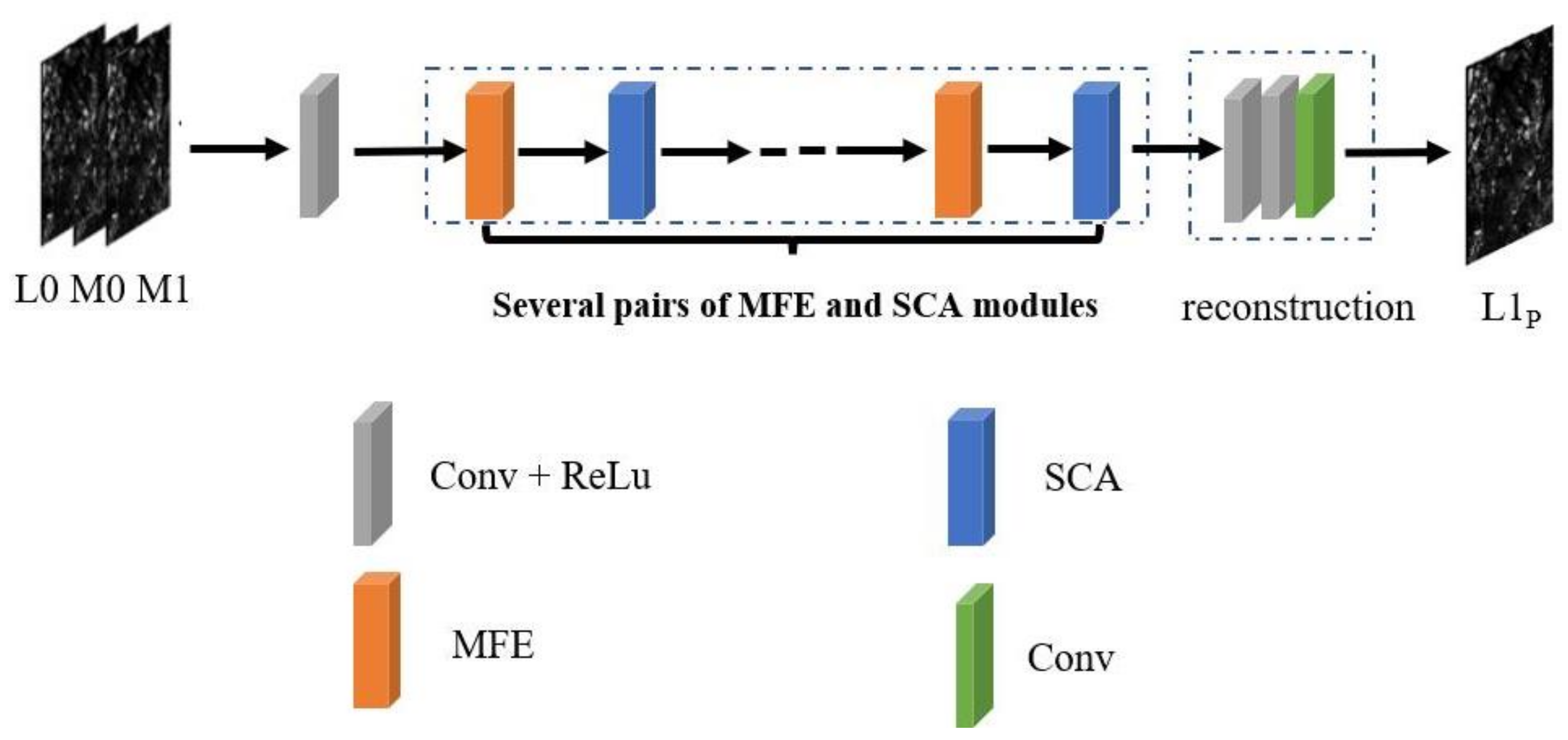
As shown in Figure 1, the proposed method can be expressed as:

$$L{1}_p=M_{re}(M_{SCA}\left(M_{MFE}\left(Cov(L0,MO,M1)\right)\right)...)$$

(1)

where $M_{re}(.)$ denotes the reconstruction operation—that is, the 3-layer two-dimensional convolution operation. $M_{SCA}(.)$ denotes the spatial and channel attention. $M_{MFE}(.)$ represents the multiscale feature extraction. $Conv(.)$ denotes the convolution operation. $...$ denotes repeating the following operations several times. After connecting $L1$, $M0$, and $M1$ in the channel dimensions, they are used as inputs to perform shallow feature extraction through a layer of convolution; after that, they use the MFE module to extract more complex features. Then, the extracted complex features are captured by the SCA to obtain the relationship between the space and the relationship between the channels to obtain better spectral quality and spatial features. Finally, the fusion image is obtained through the reconstruction operation.

The existing spatiotemporal fusion methods all use the spatial information of high-resolution images $L0$ from the reference date and the temporal information of low-resolution images $M0$ and $M1$ [7]. Because the spatial information that $M0$ and $M1$ can provide is very limited, most of the details in the final generated image should come from the “fine” image $L0$ of the reference date, so it is important to maintain the high-frequency information in $L0$ and extract more features. Deep high-resolution representation learning for human pose estimation (HRNET) [44] maintains the resolution across the entire network and achieves good results. Therefore, the proposed model does not use the classical structure of downsampling, upsampling, and image reconstruction, but rather maintains the resolution in the whole network structure to obtain as much high-frequency information as possible.

3.2. Multiscale Feature Extraction Block

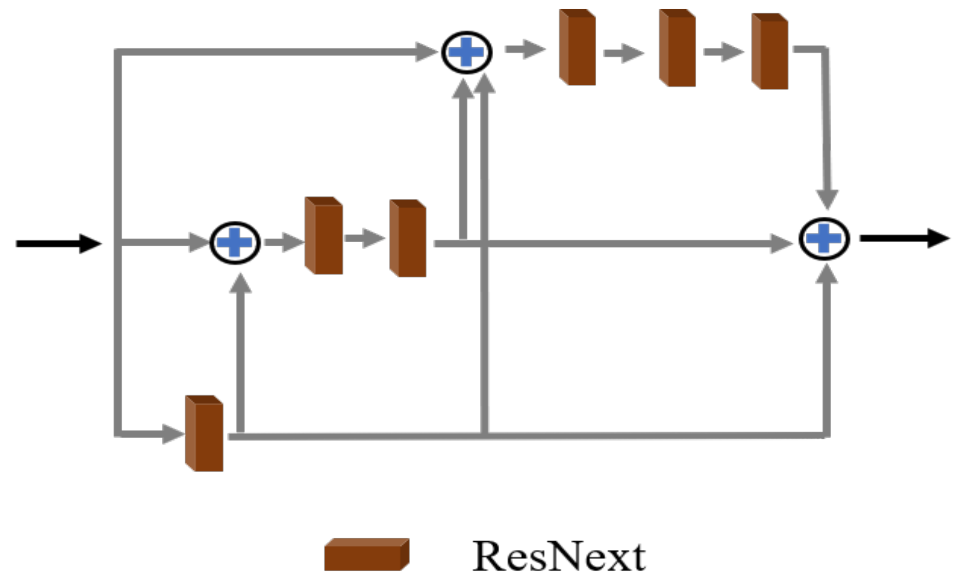
Inspired by Inception and feature pyramid networks for object detection (FPN) [45], we designed a multi-scale feature extraction module with stronger feature extraction capabilities. As Figure 2 shows, MFE has three branches. From bottom to top, rgw branches use 1, 2, and 3 ResNext modules, respectively. The more residual blocks are used, the deeper the network is. The deeper the network is, the larger the perception field is, and the richer the feature semantic information is, the less texture details will be retained [45]. To retain more semantic information and texture information at the same time, we sum the features with a smaller perceptual field of view extracted by a branch and the input as a new input and use more residual modules to obtain features with a larger perceptual field of view. Finally, the sum of the features with different perception fields extracted from the three branches is used as the output.

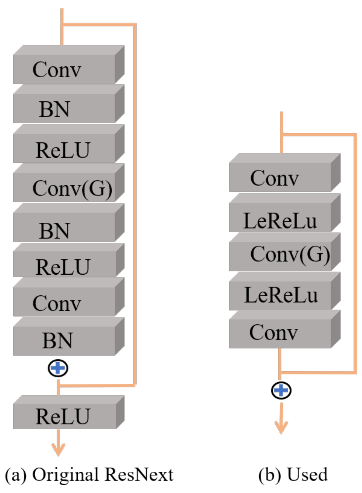
ResNext improves the residual block of ResNet to obtain a better performance with fewer parameters. Therefore, many computer vision tasks use the structure shown in Figure 3a. However, the network structure is designed for high-level visual tasks of image recognition and cannot be directly applied to low-vision tasks such as image fusion. In order to make the residual network more suitable for a spatiotemporal fusion task, we made the following changes: (1) The batch normalization (BN) layer is removed. Although the regularization method helps to train the deep network and accelerate the convergence, it may destroy the original contrast information of the image, resulting in poor fusion results [35]. (2) The activation part after summation is deleted and leaky-Relu is selected as the active function. In the residual network, it is very important to avoid changing the signal transmission of the identity mapping process, so we delete the activation operation after the summation operation. In the residual module, Leaky-ReLU is more friendly to negative signals than ReLu, so it is selected as the activation function [46].

3.3. Spatial Channel Attention Block

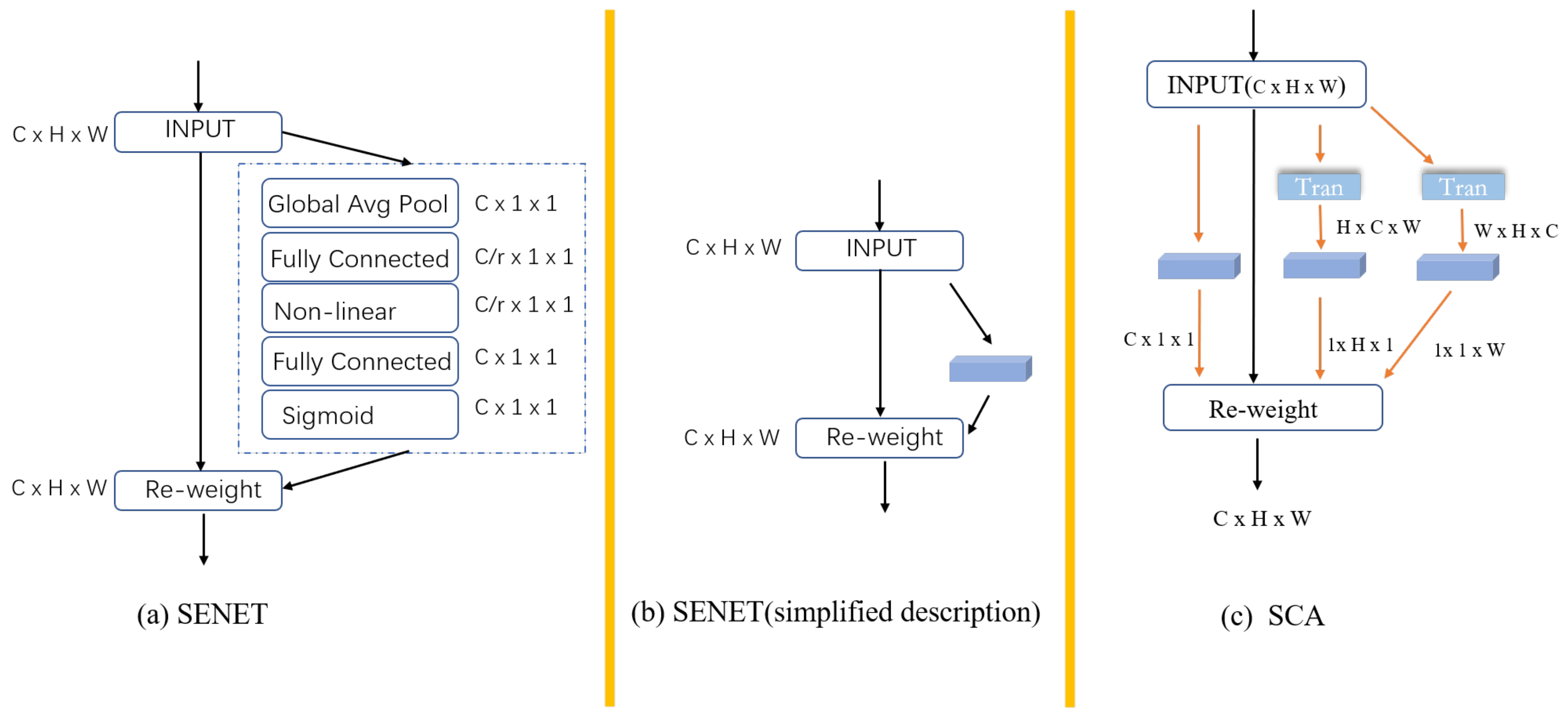
Attention mechanism have a wide range of applications to improve performance in computer vision tasks, such as pan sharpening and super-resolution. We try to use the attention mechanism to improve the results of spatiotemporal fusion. Channel attention only considers the relationship between channels and ignores the relationship between spatial locations. The relationship between rows in an image is not completely independent, the relationship between columns should not be completely independent, and this spatial location information is crucial for improving the quality of fused images. Therefore, the use of the SCA module for acquiring spatial location information at a small cost while learning inter-channel relationships is proposed. An observer can view an object from three different perspectives: front, left, and top. Similar to the observer, SCA obtains the relationships between rows, columns, and channels in three dimensions: height, width, and channels. The attention mechanism SENET, which has become very popular under computational power constraints, is used to obtain the relationships in a certain dimension, and it offers significant performance gains in exchange for lower computational costs. Figure 4a shows the SENET working mechanism in detail. If the process of capturing channel relationships is abstracted as a blue module, SENET can be depicted as shown in Figure 4b. Figure 4c shows the SCA mechanism in detail: the relationship acquisition between channels is consistent with SENET; the dimensional order of the input is changed; and then the squeeze-and-excitation mechanism is used to learn the weights between rows, the weights between columns, and the weights between channels. Finally, these three weights are multiplied with the input to obtain the result.

3.4. Compound Loss Function

The loss function is also an important factor affecting the fusion result. Using only a simple single loss function, such as $MSE$ or $L1$, it is difficult to optimize the parameters well and obtain a high-quality fusion image. Using only the $MSE$ loss function will generate a relatively smooth fusion image and will lead to losing a lot of edge information, because it is sensitive to larger outliers but not so sensitive to smaller outliers. Using $L1$ loss alone can lead to insufficient training and severe spectral noise. Some researchers have tried to use a compound loss function including perceptual loss [47] and achieved good results. However, this requires the help of a specific pre-training network, which requires additional time costs, while the result of image reconstruction also depends on the quality of the pre-trained network. In response to the above problems, we propose a novel compound loss function as Equation (2).

$$L_p=k{L}_{mse}+(1-k)L_1+\alpha L_{ssim}$$

(2)

where K is the weight factor of $L1$ loss, which changes with the advance of the training. The initial value is 0, which is equivalent to using $L_1+\alpha L_{ssim}$ to optimize rgw network. With the increase in training, k gradually increases to 1, which represents the use of $L_{mse}+\alpha L_{ssim}$ for the optimization of the network. In the experiment, each batch was set to grow by $0.02$. $\alpha$ is a factor that controls the weight of $L_{ssim}$ loss, which is set to $0.8$ based on experience. The structural similarity (SSIM) [48] index comprehensively evaluates the similarity of two images from the brightness, contrast, and structure. Multi-scale structural similarity (MS-SSIM) has a higher accuracy by evaluating SSIM at a multi-scale level. MS-SSIM is often used as an evaluation index in image reconstruction models, and its value is from 0 to 1. The closer it is to 1, the more similar the two images are [49]. It can be expressed as Equation (3):

$$L_{ssim}=1-MS\text{-}SSIM$$

(3)

SSIM can be denoted as Equation (4),

$$SSIM(x,y)=\frac{\left(2{\delta }_x{\delta }_y+C_1\right)\left(2{\eta }_{xy}+C_2\right)}{\left({\delta }_x^2+{\delta }_y^2+C_1\right)\left({\eta }_x^2+{\eta }_y^2+C_2\right)}$$

(4)

where x and y represent the target image and the predicted image, respectively; ${\delta }_x$ and ${\delta }_y$ are the mean values of the target image and the predicted image, respectively; ${\eta }_x^2$ and ${\eta }_y^2$ are the variances of the image; ${\eta }_{xy}$ represents the covariance of the image x and y; $C_1$ and $C_2$ are two variables that maintain the stability.

4. Experiments

4.1. Datasets

A classic scene in spatiotemporal data fusion is the fusion of Landsat and MODIS images. Landsat images have a spatial resolution of 30 m and a return visit time of 16 days [50]. MODIS can cover most of the Earth every day, but it obtains data with a spatial resolution of only 250 to 1000 m [50]. In this experiment, the LEVEL-2 product of Landsat 8 OLI (which has undergone preliminary radiation calibration and atmospheric correction) and the 8-day composite data MOD09A1 of MODIS are used, and the four bands of blue, green, red, and near-infrared (NIR) are used for fusion. To verify the generality of the proposed model, we selected areas in Shandong and Guangdong for experiments. Guangdong is in a coastal area, and its humid climate makes the surface of the region covered by clouds most of the time, so there are few data available for reference use after screening. The climate of Shandong is relatively drier than that of Guangdong and more cloud-free or less cloudy images are available, meaning that the dataset of Shandong is of higher quality and the heterogeneity is lower compared with that of Guangdong. For the study area in Shandong, the coordinates in the Landsat Global Reference System (WRS) are represented as $P122R034$ and the area corresponding to $h27v05$ in the MODIS Sinusoidal Tile Grid. For the study area in Guangdong, the coordinates in the WRS are represented as $P123R043$ and the area corresponding to $h28v06$ in the MODIS Sinusoidal Tile Grid. The image selection period is from 1 January 2013 to 31 December 2017. The Landsat 8 image requires a cloud coverage rate of less than $5\%$, and each scene is cropped to a size of $4800\times 4800$ (to avoid the part at the edge with no data). Considering that there are more eligible MODIS data, we choose the one closest to the date of Landsat image acquisition. The corresponding MODIS image is reprojected with a spatial resolution of 480 m and then cropped to the same area as the Landsat image with an image size of $300\times 300$. The cropped Landsat image and the corresponding MODIS image are a data pair. Finally, the Landsat and MODIS data pairs are grouped, with each group containing two Landsat and two MODIS images. Fourteen groups are chosen for each area, and the groups are then randomly divided into a training set and a test set. The training set is 10 sets of data, and the test set is 4 sets of data (the Landsat image data can be downloaded at https://earthexplorer.usgs.gov/; the MODIS image data can be downloaded at https://ladsweb.modaps.eosdis.nasa.gov/search/order/4/MOD09A1--61/2013-01-01..2017-12-31/DB/).

4.2. Experiment Settings

We use the following spatiotemporal fusion methods as references, including STARFM based on the weighted function algorithm, FSDAF based on hybrid, DCSTFN, AMNet, and EDCSTFN.

For quantitative evaluation, the following indicators are used to measure the results: spectral angle mapper (SAM) [51], relative dimensionless integrated global error (ERGAS) [52], correlation coefficient (CC), and MS-SSIM. Among these, the closer the SAM and ERGAS indexes are to 0, the closer the fusion image is to the real image. The closer the CC and MS-SSIM indicators are to 1, the closer the fusion image is to the real image.

Input settings: M0 and M1 are upsampled to the same resolution as the Landsat image using a bilinear interpolation method, and then with $L1$ in the channel dimension Concat as an input.

Network settings: The size of the convolution kernel in the “Conv + ReLu” module is 3, the step size is 1, and the output channel is 24. Three pairs of MFE and SCA are used. In the MFE module, all ResNext networks use the same settings. The three convolution operations of the ResNext network are as follows: cov (24, 30, 1), cov (30, 30, 3, g = 10), and cov (30, 24, 1). The parameters in brackets represent the input channel, output channel, and convolution core size in turn. G is the number of group convolutions. In the SCA module, the squeeze multiplier of SENET is set to 4 in the target inter-channel relationship branch. The squeeze multiplier of SENET in both the target inter-row relationship and target inter-column relationship branches is set to 32. The reconstruction module uses three-layer convolution; the convolution core size is 3; and the channels are set to 24, 12, and 4, respectively.

Training and testing settings: Inputting the entire image into the network for processing requires a large memory, which is unnecessary and not economical. It is economical and feasible to divide MODIS and Landsat images into small patch input networks in combination with hardware conditions. The patch size during training is set to 30, and the sliding step size is set to 25. The patch size during prediction is set to 30, and the sliding step size is set to 30. The initial learning rate is set to $0.001$, and a total of 70 epochs are trained. To optimize the network training parameters, we choose the Adam optimized stochastic gradient descent method. The experiment is implemented using PyTorch, and all experiments are performed with the same two GeForce RTX 2080Ti GPUs.

4.3. Results and Discussion

4.3.1. Quantitative Evaluation Comparison

The average value of each evaluation index of the fusion results is calculated separately and used as a representative of the method performance. The evaluation results of the Shandong dataset are shown in

Table 1. Quantitative assessment of different spatiotemporal fusion methods for the Shandong dataset.

Method	SAM	ERGAS	CC	SSIM
STARFM	15.4670	4.6295	0.5015	0.4190
FSDAF	13.2381	5. 0802	0.5086	0.4875
DCSTFN	7.48822	12.8310	0.6221	0.5795
AMNet	6.5622	7.3988	0.6989	0.6802
EDCSTFN	4.5044	7.2595	0.7338	0.7656
Proposed	4.1487	4.1963	0.7554	0.7922

, and the evaluation results of the Guangdong dataset are shown in

Table 2. Quantitative assessment of different spatiotemporal fusion methods for the Guangdong dataset.

Method	SAM	ERGAS	CC	SSIM
STARFM	13.7664	10.7797	0.3931	0.4337
FSDAF	12.9959	13.1992	0.3659	0.4186
DCSTFN	4.25483	8.89167	0.7449	0.8021
AMNet	3.5521	5.1040	0.7761	0.8466
EDCSTFN	3.7535	8.0302	0.7790	0.8339
Proposed	3.3246	5.0842	0.7862	0.8646

.

From Table 1 and Table 2, it is easy to find that the fusion results of FSDAF are better than those of STARFM, which may be due to the better performance results of FSDAF for heterogeneous regions. DCSTFN has a larger improvement than FSDAF, which may benefit from the stronger representation capability of CNN. The relationship between the input and output in AMNet and EDCSTFN models is completely learned by the network, rather than based on some assumptions; thus, there is a more significant improvement in the fusion results compared to DCSTFN. AMNet performs better than EDCSTFN in the Shandong dataset, but AMNet slightly outperforms EDCSTFN in the Guangdong region, probably due to the contrast caused by the complexity of the topography in the Guangdong dataset. The proposed method uses the MFE and SCA modules to effectively analyze the complex spatial information of the images and capture inter-channel information, which plays a positive role in the fusion results; therefore, it performs better in objective metrics.

4.3.2. Visual Comparison

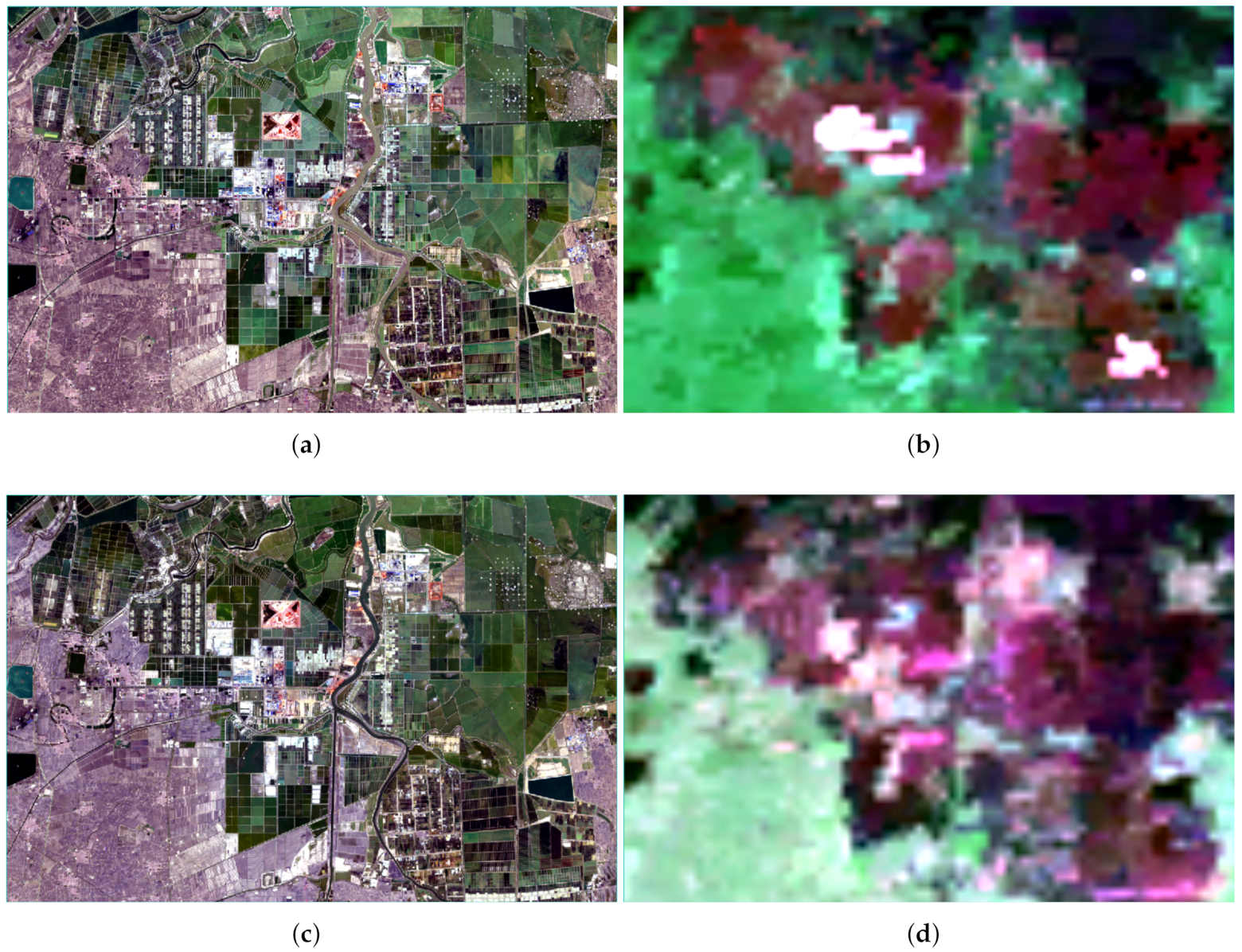
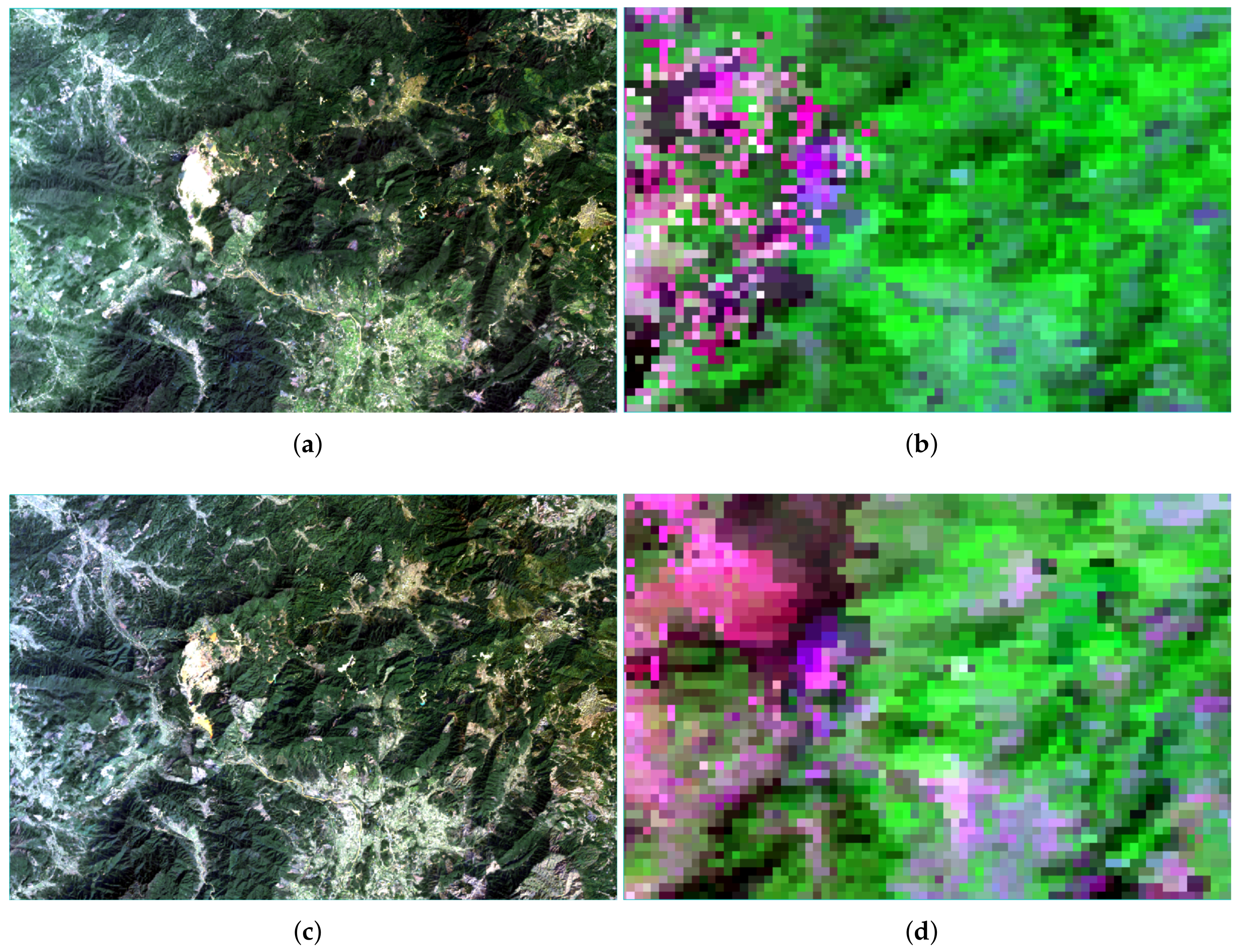
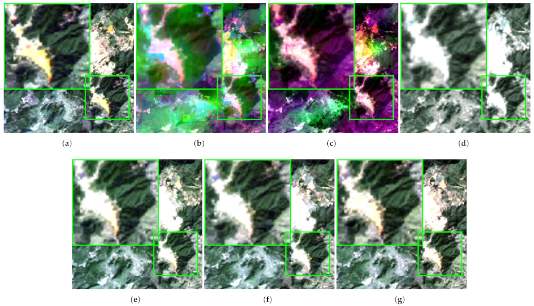
In order to visualize the performance comparison of each algorithm, we intercepted the same area of $300\times 300$ in the fusion results of different algorithms under the same test case and magnified the area of $100\times 100$ twice to compare the details. To verify the performance and robustness of the method, we selected areas with different land cover types on different data sets; the selected areas had rich color information and texture information. For the Shandong dataset, we selected a building area with rich spectral information; for the Guangdong dataset, we selected a mountainous area with rich spectral information. For the Shandong region, Figure 5 shows a sample with time 20160310 as the reference data and time 20160326 as the target data, and the fusion results were compared as shown in Figure 6. For the Guangdong region, Figure 7 shows a sample with time 20141015 as the reference data and time 20150119 as the target data, and the fusion results are compared as shown in Figure 8.

From the zoomed area in the upper left corner of the fusion results in Figure 6, it can be clearly seen that STARFM and FSDAF are richer in their color performance but poorer in texture details, and there are large differences with the real image. In particular, STARFM has obvious mosaic patches. DCSTFN, AMNet, and EDCSTFN are better at retaining texture information, but they all exhibit a “lighter” color representation. Our proposed method not only retains texture details better but also is closer to the real image in terms of spectral information.

It is easy to see from the enlarged area in the upper left corner of the fusion results of each experiment in Figure 8: STARFM and FSADF are equally bad in terms of texture information retention, and STARFM can barely see the texture information. In DCSTFN, AMNet, and EDCSTFN, the texture information is well preserved and the mountain contours can be seen, but DCSTFN has almost no spectral information, and AMNet and EDCSTFN retain only a very small amount of information in the lower right corner. Our proposed model outperforms other algorithms in terms of both spectral information retention and texture detail retention.

In summary, the fusion results of our proposed method are closer to those of the real image, both in terms of texture detail information and spectral information.

4.3.3. Computational Efficiency Comparison

We compared the DNN-based models in the benchmark experiments in two dimensions, model parameters and floating points of operations (FLOPs); the results are shown in

Table 3. Comparison of model computational efficiency.

Method	Parameters	FLOPs (G)
DCSTFN	408,961	150.481
AMNet	633,452	97.974
EDCSTFN	281,764	64.918
Proposed	133,420	10.684
Reference	↓	↓

. Parameters represent the number of parameters that the model needs to learn. In FLOPs(G), G represents $1\times {10}^6$, and FLOPs is used to measure the computational complexity of the model. From Table 3, we can find that our proposed model is much lower than the other methods in terms of the number of parameters and FLOPs, where the number of parameters is only half that of EDCSTFN and the difference between FLOPs and DCSTFN is more than 10 times. It can be considered that our proposed model is more advantageous in terms of its computational complexity.

4.3.4. Comparison of Residual Graphs

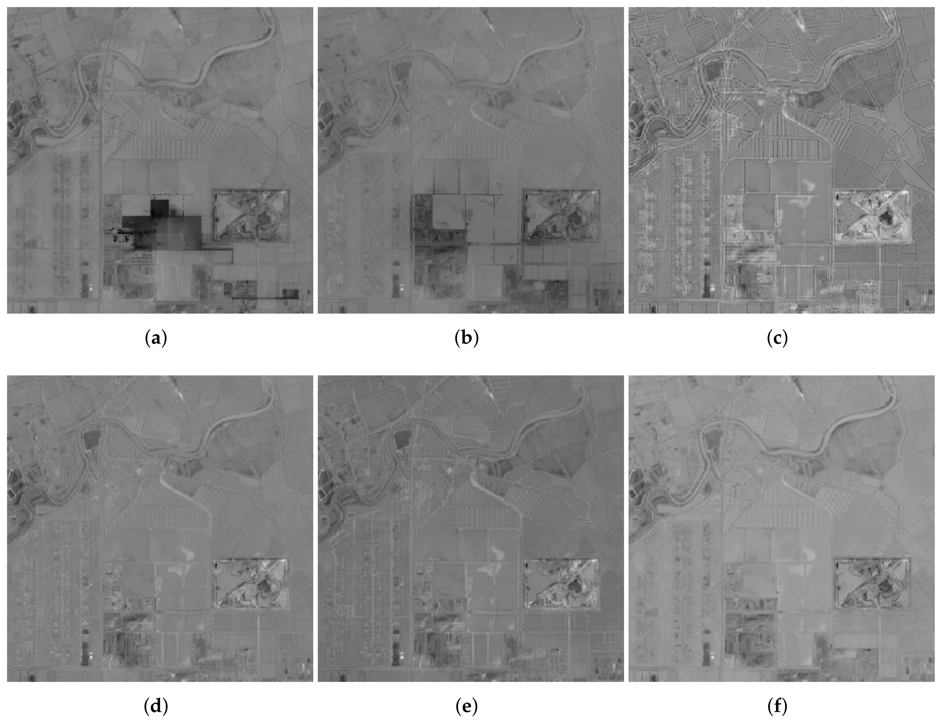
To further verify the effectiveness of the proposed method, the residual image experiment is set up by selecting regions in the visual comparison experiment. The residual image is the real image subtracted from the fused image pixel by pixel, and the average value of each band is taken. Theoretically, the closer the fused image is to the real image, the less content appears on the residual image. The results of the comparison of residual image for the Shandong and Guangdong datasets are shown in Figure 9 and Figure 10, respectively. As can be seen in Figure 9, the residual map of the proposed method has less texture. In Figure 10, the residual maps of the last three DNN-based methods are similar, and a closer look shows that the residual maps of our proposed method are generally smoother, meaning that the proposed method has the best fusion effect. In general, the DNN-based methods generally outperform the traditional algorithms.

4.3.5. Ablation Experiments

We performed ablation experiments on the Guangdong data set to demonstrate the effectiveness of the proposed module. To verify the effect of each module, we first designed the basic network structure as a comparison. The basic network uses SENET instead of the proposed SCA module, and the loss function is $L1$ + $L_{ssim}$. $L_p$ represents the compound loss function we proposed. +BN means adding the BN layer to the network, +SCA means replacing SENET with the proposed SCA module, and +$L_p$ means replacing the loss function in the base network with the proposed loss function. the results are shown in

Table 4. Performance evaluation of different module structures on the Guangdong dataset.

ID	Method	SAM	ERGAS	CC	SSIM
1	Base	3.3795	4.9559	0.7811	0.8531
2	Base + BN	3.6224	4.5479	0.7732	0.8494
3	Base + SCA	3.4346	4.5991	0.7841	0.861
4	Base + SCA + $L_p$	3.3246	5.0842	0.7862	0.8646

.

From the comparison of experiment 1 and experiment 2, it can be found that the BN layer is not suitable for spatiotemporal fusion tasks because it destroys the internal connection of the image. The comparison of experiment 1 and experiment 3 can verify that the SCA module can acquire certain spatial information while learning the relationship between channels, thereby improving the performance. The comparison between experiment 3 and experiment 4 can verify that the proposed composite loss function can more effectively optimize the network and improve its performance.

4.3.6. Sensitivity of the Method to the Amount of Training Data

To explore the sensitivity of the proposed method to the training data, we compared the performance of AMNet, EDCSTFN, and the proposed method with 3, 5, and 8 sets of training data, respectively, on the Shandong dataset. The comparison results are shown in

Table 5. Quantitative assessment of different algorithms using 3 sets of training data in the Shandong dataset.

Method	SAM	ERGAS	CC	SSIM
AMNet	4.9110	7.2776	0.7199	0.7360
EDCSTFN	4.8423	9.9645	0.7274	0.7296
Proposed	4.8621	7.2593	0.7267	0.7437

,

Table 6. Quantitative assessment of different algorithms using 5 sets of training data in the Shandong dataset.

Method	SAM	ERGAS	CC	SSIM
AMNet	4.7582	7.5967	0.7294	0.7583
EDCSTFN	4.5671	6.9118	0.7362	0.7587
Proposed	4.4496	5.4320	0.7518	0.7939

and

Table 7. Quantitative assessment of different algorithms using 8 sets of training data in the Shandong dataset.

Method	SAM	ERGAS	CC	SSIM
AMNet	7.8941	10.6959	0.6721	0.6390
EDCSTFN	4.2838	6.5594	0.7388	0.7676
Proposed	4.3316	6.0588	0.7453	0.7841

.

From Table 1 and Table 5, Table 6 and Table 7, it can be seen that in the case of different training groups, the performance of DNN-based methods has different degrees of impact, and the proposed method has considerable competitiveness. The corresponding data for each algorithm in Table 5 and Table 6 show that the performance obtained using five sets of training data is better than that obtained using three sets of training data, where the proposed method has the largest increase, probably because three sets of training data are too few for the method, which limits its performance. The corresponding data for AMNet in Table 6 and Table 7 have large fluctuations, while EDCSTFN and the proposed method show only small changes. From Table 1 and Table 7, it can be found that the performance of each algorithm fluctuates less.

4.4. Discussion

The experimental data of the Shandong and Guangdong regions shows that our proposed model has a better prediction accuracy and better visual effects than other methods. The regional geologies of Shandong and Guangdong are quite different, and the proposed model still maintains a good performance, which shows that it has better robustness. These superiorities may be due to the fact that the multiscale mechanism can extract more complex features and the attention mechanism focuses on both the relationships between channels and the spatial relationships. In the proposed method, the relationship between the fusion result and the input is obtained entirely by the network learning, without relying on specific assumptions. The proposed method can effectively capture spectral information and texture features.

Despite these improvements in our approach, there are still some areas where our work could be improved. The quality of the dataset is not high enough. For example, in areas such as Guangdong, dates in the majority of the year have cloud coverage, and it is difficult to collect enough high-quality data. In addition, there is limited ability to capture changes in scenarios where the land cover changes drastically in a short period of time. In the future, we will consider the better preprocessing of the data, such as cloud processing, and at the same time will work to collect higher-quality data and investigate methods to better capture changes.

5. Conclusions

In this paper, a multiscale mechanism that can learn complex features in image is used, and the use of a novel attention mechanism for capturing both spatial and channel information is proposed. Additionally, the use of a new composite loss function which can successfully obtain higher-quality fusion results is proposed. Comparative experiments on different regional datasets as well as ablation experiments validate the effectiveness of this method. Future work will continue to focus on the retention of structural information and additionally consider the use of Generative Adversarial Network (GAN) structures for spatiotemporal fusion.

References

1. Toth, C.; Jóźków, G. Remote sensing platforms and sensors: A survey. ISPRS J. Photogramm. Remote Sens. 2016, 115, 22–36. [Google Scholar] [CrossRef]
2. Di, L. Geospatial sensor web and self-adaptive Earth predictive systems (SEPS). In Proceedings of the Earth Science Technology Office (ESTO)/Advanced Information System Technology (AIST) Sensor Web Principal Investigator (PI) Meeting, San Diego, CA, USA, 13–14 February 2007; pp. 1–4. [Google Scholar]
3. Kalajdjieski, J.; Zdravevski, E.; Corizzo, R.; Lameski, P.; Kalajdziski, S.; Pires, I.M.; Garcia, N.M.; Trajkovik, V. Air pollution prediction with multi-modal data and deep neural networks. Remote Sens. 2020, 12, 4142. [Google Scholar] [CrossRef]
4. Li, Z.; Yang, X. Fusion of High-and Medium-Resolution Optical Remote Sensing Imagery and GlobeLand30 Products for the Automated Detection of Intra-Urban Surface Water. Remote Sens. 2020, 12, 4037. [Google Scholar] [CrossRef]
5. Xu, K.; Zhang, J.; Li, H.; Cao, W.; Zhu, Y.; Jiang, X.; Ni, J. Spectrum-and RGB-D-Based Image Fusion for the Prediction of Nitrogen Accumulation in Wheat. Remote Sens. 2020, 12, 4040. [Google Scholar] [CrossRef]
6. Amorós-López, J.; Gómez-Chova, L.; Alonso, L.; Guanter, L.; Zurita-Milla, R.; Moreno, J.; Camps-Valls, G. Multitemporal fusion of Landsat/TM and ENVISAT/MERIS for crop monitoring. Int. J. Appl. Earth Obs. Geoinf. 2013, 23, 132–141. [Google Scholar] [CrossRef]
7. Zhu, X.; Helmer, E.H.; Gao, F.; Liu, D.; Chen, J.; Lefsky, M.A. A flexible spatiotemporal method for fusing satellite images with different resolutions. Remote Sens. Environ. 2016, 172, 165–177. [Google Scholar] [CrossRef]
8. Chen, B.; Huang, B.; Xu, B. Comparison of spatiotemporal fusion models: A review. Remote Sens. 2015, 7, 1798–1835. [Google Scholar] [CrossRef] [Green Version]
9. Duan, P.; Kang, X.; Ghamisi, P.; Liu, Y. Multilevel Structure Extraction-Based Multi-Sensor Data Fusion. Remote Sens. 2020, 12, 4034. [Google Scholar] [CrossRef]
10. Hilker, T.; Wulder, M.A.; Coops, N.C.; Seitz, N.; White, J.C.; Gao, F.; Masek, J.G.; Stenhouse, G. Generation of dense time series synthetic Landsat data through data blending with MODIS using a spatial and temporal adaptive reflectance fusion model. Remote Sens. Environ. 2009, 113, 1988–1999. [Google Scholar] [CrossRef]
11. Belgiu, M.; Stein, A. Spatiotemporal image fusion in remote sensing. Remote Sens. 2019, 11, 818. [Google Scholar] [CrossRef] [Green Version]
12. Gao, F.; Masek, J.; Schwaller, M.; Hall, F. On the blending of the Landsat and MODIS surface reflectance: Predicting daily Landsat surface reflectance. IEEE Trans. Geosci. Remote Sens. 2006, 44, 2207–2218. [Google Scholar]
13. Zhu, X.; Cai, F.; Tian, J.; Williams, T.K.A. Spatiotemporal fusion of multisource remote sensing data: Literature survey, taxonomy, principles, applications, and future directions. Remote Sens. 2018, 10, 527. [Google Scholar] [CrossRef] [Green Version]
14. Zhu, X.; Chen, J.; Gao, F.; Chen, X.; Masek, J.G. An enhanced spatial and temporal adaptive reflectance fusion model for complex heterogeneous regions. Remote Sens. Environ. 2010, 114, 2610–2623. [Google Scholar] [CrossRef]
15. Emelyanova, I.V.; McVicar, T.R.; Van Niel, T.G.; Li, L.T.; Van Dijk, A.I. Assessing the accuracy of blending Landsat–MODIS surface reflectances in two landscapes with contrasting spatial and temporal dynamics: A framework for algorithm selection. Remote Sens. Environ. 2013, 133, 193–209. [Google Scholar] [CrossRef]
16. Tan, Z.; Yue, P.; Di, L.; Tang, J. Deriving high spatiotemporal remote sensing images using deep convolutional network. Remote Sens. 2018, 10, 1066. [Google Scholar] [CrossRef] [Green Version]
17. Zhukov, B.; Oertel, D.; Lanzl, F.; Reinhackel, G. Unmixing-based multisensor multiresolution image fusion. IEEE Trans. Geosci. Remote Sens. 1999, 37, 1212–1226. [Google Scholar] [CrossRef]
18. Wu, M.; Niu, Z.; Wang, C.; Wu, C.; Wang, L. Use of MODIS and Landsat time series data to generate high-resolution temporal synthetic Landsat data using a spatial and temporal reflectance fusion model. J. Appl. Remote Sens. 2012, 6, 063507. [Google Scholar]
19. Wu, M.; Huang, W.; Niu, Z.; Wang, C. Generating daily synthetic Landsat imagery by combining Landsat and MODIS data. Sensors 2015, 15, 24002–24025. [Google Scholar] [CrossRef] [Green Version]
20. Li, X.; Foody, G.M.; Boyd, D.S.; Ge, Y.; Zhang, Y.; Du, Y.; Ling, F. SFSDAF: An enhanced FSDAF that incorporates sub-pixel class fraction change information for spatio-temporal image fusion. Remote Sens. Environ. 2020, 237, 111537. [Google Scholar] [CrossRef]
21. Cammalleri, C.; Anderson, M.; Gao, F.; Hain, C.; Kustas, W. Mapping daily evapotranspiration at field scales over rainfed and irrigated agricultural areas using remote sensing data fusion. Agric. For. Meteorol. 2014, 186, 1–11. [Google Scholar] [CrossRef] [Green Version]
22. Shen, H.; Huang, L.; Zhang, L.; Wu, P.; Zeng, C. Long-term and fine-scale satellite monitoring of the urban heat island effect by the fusion of multi-temporal and multi-sensor remote sensed data: A 26-year case study of the city of Wuhan in China. Remote Sens. Environ. 2016, 172, 109–125. [Google Scholar] [CrossRef]
23. Xia, H.; Chen, Y.; Li, Y.; Quan, J. Combining kernel-driven and fusion-based methods to generate daily high-spatial-resolution land surface temperatures. Remote Sens. Environ. 2019, 224, 259–274. [Google Scholar] [CrossRef]
24. Li, Z.; Huang, C.; Zhu, Z.; Gao, F.; Tang, H.; Xin, X.; Ding, L.; Shen, B.; Liu, J.; Chen, B.; et al. Mapping daily leaf area index at 30 m resolution over a meadow steppe area by fusing Landsat, Sentinel-2A and MODIS data. Int. J. Remote Sens. 2018, 39, 9025–9053. [Google Scholar] [CrossRef]
25. Huang, B.; Song, H. Spatiotemporal reflectance fusion via sparse representation. IEEE Trans. Geosci. Remote Sens. 2012, 50, 3707–3716. [Google Scholar] [CrossRef]
26. Chen, B.; Huang, B.; Xu, B. A hierarchical spatiotemporal adaptive fusion model using one image pair. Int. J. Digit. Earth 2017, 10, 639–655. [Google Scholar] [CrossRef]
27. Wei, J.; Wang, L.; Liu, P.; Chen, X.; Li, W.; Zomaya, A.Y. Spatiotemporal fusion of MODIS and Landsat-7 reflectance images via compressed sensing. IEEE Trans. Geosci. Remote Sens. 2017, 55, 7126–7139. [Google Scholar] [CrossRef]
28. Lacey, G.; Taylor, G.W.; Areibi, S. Deep learning on fpgas: Past, present, and future. arXiv 2016, arXiv:1602.04283. [Google Scholar]
29. Liu, W.; Wang, Z.; Liu, X.; Zeng, N.; Liu, Y.; Alsaadi, F.E. A survey of deep neural network architectures and their applications. Neurocomputing 2017, 234, 11–26. [Google Scholar] [CrossRef]
30. Voulodimos, A.; Doulamis, N.; Doulamis, A.; Protopapadakis, E. Deep learning for computer vision: A brief review. Comput. Intell. Neurosci. 2018, 2018, 7068349. [Google Scholar] [CrossRef] [PubMed]
31. Song, H.; Liu, Q.; Wang, G.; Hang, R.; Huang, B. Spatiotemporal satellite image fusion using deep convolutional neural networks. IEEE J. Sel. Top. Appl. Earth Obs. Remote Sens. 2018, 11, 821–829. [Google Scholar] [CrossRef]
32. Liu, X.; Deng, C.; Chanussot, J.; Hong, D.; Zhao, B. StfNet: A two-stream convolutional neural network for spatiotemporal image fusion. IEEE Trans. Geosci. Remote Sens. 2019, 57, 6552–6564. [Google Scholar] [CrossRef]
33. Jia, D.; Song, C.; Cheng, C.; Shen, S.; Ning, L.; Hui, C. A Novel Deep Learning-Based Spatiotemporal Fusion Method for Combining Satellite Images with Different Resolutions Using a Two-Stream Convolutional Neural Network. Remote Sens. 2020, 12, 698. [Google Scholar] [CrossRef] [Green Version]
34. Li, W.; Zhang, X.; Peng, Y.; Dong, M. Spatiotemporal fusion of remote sensing images using a convolutional neural network with attention and multiscale mechanisms. Int. J. Remote Sens. 2021, 42, 1973–1993. [Google Scholar] [CrossRef]
35. Tan, Z.; Di, L.; Zhang, M.; Guo, L.; Gao, M. An Enhanced Deep Convolutional Model for Spatiotemporal Image Fusion. Remote Sens. 2019, 11, 2898. [Google Scholar] [CrossRef] [Green Version]
36. He, K.; Zhang, X.; Ren, S.; Sun, J. Deep residual learning for image recognition. In Proceedings of the IEEE Conference on Computer Vision and Pattern Recognition, Las Vegas, NV, USA, 27–30 June 2016; pp. 770–778. [Google Scholar]
37. Xie, S.; Girshick, R.; Dollár, P.; Tu, Z.; He, K. Aggregated residual transformations for deep neural networks. In Proceedings of the IEEE Conference on Computer Vision and Pattern Recognition, Honolulu, HI, USA, 21–26 July 2017; pp. 1492–1500. [Google Scholar]
38. Szegedy, C.; Ioffe, S.; Vanhoucke, V.; Alemi, A. Inception-v4, inception-resnet and the impact of residual connections on learning. In Proceedings of the AAAI Conference on Artificial Intelligence, San Francisco, CA, USA, 4–9 February 2017; Volume 31. [Google Scholar]
39. Chollet, F. Xception: Deep learning with depthwise separable convolutions. In Proceedings of the IEEE Conference on Computer Vision and Pattern Recognition, Honolulu, HI, USA, 21–26 July 2017; pp. 1251–1258. [Google Scholar]
40. Hu, J.; Shen, L.; Sun, G. Squeeze-and-excitation networks. In Proceedings of the IEEE Conference on Computer Vision and Pattern Recognition, Salt Lake City, UT, USA, 18–23 June 2018; pp. 7132–7141. [Google Scholar]
41. Park, J.; Woo, S.; Lee, J.Y.; Kweon, I.S. Bam: Bottleneck attention module. arXiv 2018, arXiv:1807.06514. [Google Scholar]
42. Woo, S.; Park, J.; Lee, J.Y.; Kweon, I.S. Cbam: Convolutional block attention module. In Proceedings of the European Conference on Computer Vision (ECCV), Munich, Germany, 8–14 September 2018; pp. 3–19. [Google Scholar]
43. Wang, X.; Girshick, R.; Gupta, A.; He, K. Non-local neural networks. In Proceedings of the IEEE Conference on Computer Vision and Pattern Recognition, Salt Lake City, UT, USA, 18–23 June 2018; pp. 7794–7803. [Google Scholar]
44. Sun, K.; Xiao, B.; Liu, D.; Wang, J. Deep high-resolution representation learning for human pose estimation. In Proceedings of the IEEE Conference on Computer Vision and Pattern Recognition, Long Beach, CA, USA, 15–20 June 2019; pp. 5693–5703. [Google Scholar]
45. Lin, T.Y.; Dollár, P.; Girshick, R.; He, K.; Hariharan, B.; Belongie, S. Feature pyramid networks for object detection. In Proceedings of the IEEE Conference on Computer Vision and Pattern Recognition, Honolulu, HI, USA, 21–26 July 2017; pp. 2117–2125. [Google Scholar]
46. Maas, A.L.; Hannun, A.Y.; Ng, A.Y. Rectifier nonlinearities improve neural network acoustic models. In Proceedings of the ICML, Citeseer, Atlanta, GA, USA, 16–21 June 2013; Volume 30, p. 3. [Google Scholar]
47. Johnson, J.; Alahi, A.; Fei-Fei, L. Perceptual losses for real-time style transfer and super-resolution. In European Conference on Computer Vision; Springer: Berlin/Heidelberg, Germany, 2016; pp. 694–711. [Google Scholar]
48. Wang, Z.; Bovik, A.C.; Sheikh, H.R.; Simoncelli, E.P. Image quality assessment: From error visibility to structural similarity. IEEE Trans. Image Process. 2004, 13, 600–612. [Google Scholar] [CrossRef] [Green Version]
49. Zhao, H.; Gallo, O.; Frosio, I.; Kautz, J. Loss functions for neural networks for image processing. arXiv 2015, arXiv:1511.08861. [Google Scholar]
50. Roy, D.P.; Wulder, M.A.; Loveland, T.R.; Woodcock, C.E.; Allen, R.G.; Anderson, M.C.; Helder, D.; Irons, J.R.; Johnson, D.M.; Kennedy, R.; et al. Landsat-8: Science and product vision for terrestrial global change research. Remote Sens. Environ. 2014, 145, 154–172. [Google Scholar] [CrossRef] [Green Version]
51. Yuhas, R.H.; Goetz, A.F.; Boardman, J.W. Discrimination among semi-arid landscape endmembers using the spectral angle mapper (SAM) algorithm. In Proceedings of the Summaries 3rd Annual JPL Airborne Geoscience Workshop, Pasadena, CA, USA, 1–5 June 1992; Volume 1, pp. 147–149. [Google Scholar]
52. Khan, M.M.; Alparone, L.; Chanussot, J. Pansharpening quality assessment using the modulation transfer functions of instruments. IEEE Trans. Geosci. Remote Sens. 2009, 47, 3880–3891. [Google Scholar] [CrossRef]
Figure 1. Proposed network, where Conv+ReLu represents the convolution operation followed by the ReLu activation function, SCA represents the proposed spatial channel attention module, MFE represents the proposed multiscale feature extraction module, and Conv represents the convolution operation.
Remotesensing 14 00461 g001
Figure 2. The proposed MFE module, where “⊕” denotes the element-wise sum.
Remotesensing 14 00461 g002
Figure 3. Comparison of ResNext blocks. “⊕” denotes element-wise sum, while Conv(G) denotes group convolution operation.
Remotesensing 14 00461 g003
Figure 4. SENET and the proposed SCA module, where “Tran” indicates an operation that changes the order of the input dimensions and C, H, and W represent the number of channels, height, and width of the feature map, respectively.
Remotesensing 14 00461 g004
Figure 5. A sample demonstration of the subjective performance comparison of the Shandong dataset. (a) L 0 . (b) M 0 . (c) L 1 . (d) M 1 .
Remotesensing 14 00461 g005
Figure 6. Visual evaluation of different spatiotemporal fusion methods for Shandong datasets at 20160326. (a) Ground truth. (b) STARFM. (c) FSDAF. (d) DCSTFN. (e) AMNet. (f) EDCSTFN. (g) Proposed.
Remotesensing 14 00461 g006
Figure 7. A sample demonstration of the subjective performance comparison of the Guangdong dataset. (a) L 0 . (b) M 0 . (c) L 1 . (d) M 1 .
Remotesensing 14 00461 g007
Figure 8. Visual evaluation of different spatiotemporal fusion methods for Guangdong datasets at 20150119 moment. (a) Ground truth. (b) STARFM. (c) FSDAF. (d) DCSTFN. (e) AMNet. (f) EDCSTFN. (g) Proposed.
Remotesensing 14 00461 g008
Figure 9. Comparison of residual images in Shandong 20160326 scene. (a) STARFM. (b) FSDAF. (c) DCSTFN. (d) AMNet. (e) EDCSTFN. (f) Proposed.
Remotesensing 14 00461 g009
Figure 10. Comparison of residual images in Guangdong 20150119 scene. (a) STARFM. (b) FSDAF. (c) DCSTFN. (d) AMNet. (e) EDCSTFN. (f) Proposed.
Remotesensing 14 00461 g010