Remote Sensing Pansharpening by Full-Depth Feature Fusion

Abstract

Pansharpening is an important yet challenging remote sensing image processing task, which aims to reconstruct a high-resolution (HR) multispectral (MS) image by fusing a HR panchromatic (PAN) image and a low-resolution (LR) MS image. Though deep learning (DL)-based pansharpening methods have achieved encouraging performance, they are infeasible to fully utilize the deep semantic features and shallow contextual features in the process of feature fusion for a HR-PAN image and LR-MS image. In this paper, we propose an efficient full-depth feature fusion network (FDFNet) for remote sensing pansharpening. Specifically, we design three distinctive branches called PAN-branch, MS-branch, and fusion-branch, respectively. The features extracted from the PAN and MS branches will be progressively injected into the fusion branch at every different depth to make the information fusion more broad and comprehensive. With this structure, the low-level contextual features and high-level semantic features can be characterized and integrated adequately. Extensive experiments on reduced- and full-resolution datasets acquired from WorldView-3, QuickBird, and GaoFen-2 sensors demonstrate that the proposed FDFNet only with less than 100,000 parameters performs better than other detail injection-based proposals and several state-of-the-art approaches, both visually and quantitatively.

1. Introduction

Due to the limited light energy and the sensitivity of remote sensing imaging sensors such as WorldView-3, QuickBird, and GaoFen-2, only multispectral (MS) images with low spatial-resolution (LR-MS) and panchromatic (PAN) gray-scaled image with high spatial-resolution (HR-PAN) can be obtained directly from optical devices. However, what is highly desirable in a wide range of applications, including change detection, classification, and object recognition, are images with rich spectral information and spatial details. The task of pansharpening is namely to obtain such high-resolution multispectral (HR-MS) images by fusing the known HR-PAN and LR-MS images, improving the spatial resolution of MS images while maintaining the high resolution in the spectral domain. Recently, pansharpening has been an active field of research, getting more and more attention in remote sensing image processing. The competition [1] initiated by the Data Fusion Committee of the IEEE Geoscience and Remote Sensing Society in 2006, and many recently published review papers proved the rapid development trend of pansharpening. In scientific research, pansharpening has also received extensive attention in the industry of some companies, e.g., Google Earth, DigitalGlobe, etc.

Over the past few decades, a large variety of pansharpening methods have been proposed. Most of them can be divided into the following four categories: Component substitution (CS) [2,3,4,5] approaches, multi-resolution analysis (MRA) [1,6,7,8,9,10,11] approaches, variational optimization (VO) [12,13,14,15,16,17,18,19,20,21,22,23,24,25,26,27,28,29,30,31,32,33] approaches, and deep learning (DL) approaches [34,35,36,37,38,39,40,41,42].

The main idea of the CS-based method can be summarized as replacing specific components of the LR-MS images with the HR-PAN image. To be more specific, the spatial component separated by a spectral transformation of the LR-MS image is first substituted with the PAN image, and then the sharpened image is transformed into the original domain through back projection. Among CS-based methods, most of them can produce results with satisfying spatial fidelity yet usually lead to severe spectral distortion. Some typical examples of methods that fall into this category are spatial details with local parameter estimation (BDSD) [2], spatial details with a strong dependency (BDSD-PC) method [3], and partial replacement of adaptive component substitution (PRACS) [4].

The MRA-based methods work to inject the spatial details extracted from the HR-PAN image into the LR-MS images through a multi-resolution analysis framework. Products obtained by MRA-based techniques usually retain spectral information well, but suffer from spatial distortion. Typical instances of such a class are smoothing filter-based intensity modulation (SFIM) [6], additive wavelet intensity ratio (AWLP) [7], generalized Laplacian pyramid (GLP) [1,43], with GLP with robust regression [44] and GLP with comprehensive regression (GLP-Reg) [11].

VO-based methods regard pansharpening as an inverse problem that is usually ill-posed. These methods need to describe the potential relationship among HR-PAN images, LR-MS images, and unknown HR-MS images by establishing equations, which could be solved by the designed optimization algorithms. Compared with CS and MRA methods, they can achieve a better balance between spectral fidelity and spatial fidelity, but at the cost of the increased computational burden. Technologies in this category include: Bayesian methods [14,15,16], variational methods [17,18,19,21,22,23,24,25,26,27,28,29], and compressed sensing technology [30,31,32]. Typical instances of this class are TV [20], LGC(CVPR19) [12], and DGS [13].

Recently, with the rapid development of deep learning and accessibility of high-performance computing hardware equipment, convolutional neural networks (CNNs) have shown outstanding performance in image processing fields, e.g., image resolution reconstruction [45,46,47,48,49], image segmentation [50,51,52], image fusion [53,54,55,56,57], image classification [58], image denoising [59], etc. Therefore, many methods [34,35,36,37,38,41,42,58,59,60,61,62,63,64,65,66,67,68,69,70,71,72,73,74,75] based on deep learning have also been applied to solve the pansharpening problem. Benefiting from the powerful nonlinear fitting and feature extraction capabilities of CNNs and the availability of big data, these DL-based methods could perform better than the above three methods to a certain degree, i.e., CS-, MRA-, and VO-based methods. Researchers have designed various CNNs with different structures and characteristics. Specifically, the general paradigm uses LR-MS images and HR-PAN images as input to the network. The desired HR-MS images can have output through the trained network. For example, Wei et al. [61] proposed the concept of residual learning to make full use of the high nonlinearity of deep learning models. Moreover, Yuan et al. [60] introduced multi-scale feature extraction into the basic convolutional neural network (CNN) architecture and proposed the multi-scale and multi-depth CNN for pansharpening. In 2018, Scarpa et al. [72] proposed a target-adaptive usage modality to achieve good performance in the presence of a mismatch with respect to the training set and across different sensors. In [61], the concept of residual learning was introduced by Wei et al. to form a very deep convolutional neural network to make full use of the high nonlinearity of deep learning models.

However, most of the existing CNN frameworks directly concatenate the HR-PAN image and LR-MS image together in the spectral channel dimension as the network’s input, neglecting the unique characteristics of the HR-PAN image and LR-MS images. This operation would result in the distinctive features in HR-PAN and LR-MS images that cannot be perceived and extracted effectively. Besides, there are essential differences between HR-PAN images and LR-MS images both in spatial and spectral dimensions, making the fusion procedure more difficult. In [41], Zhang et al. designed two independent branches for HR-PAN and LR-MS images to explore their features separately and finally performed feature fusion operations on their respective deep features. In this case, BDPN will fail to fuse the feature map in shallow depth and medium depth of the network, attenuating the fusion ability.

To address the above problem, we propose an efficient full-depth feature fusion network (FDFNet) for remote sensing pansharpening. The main contributions of this paper can be summarized as follows.

1.

A novel FDFNet is designed to learn the continuous features for the PAN image, MS images, and the fusion images through three branches, separately. These three branches are arranged in parallel. The transfer of feature maps and information interaction among the three branches are carried out at different depths of the network, enabling the network to generate specific representations for images of various properties and the relationships between them.

2.

The features extracted from the MS branch and PAN branch will be injected into the fusion branch at every different depth, promoting the network to characterize better and integrate the detailed low-level features and high-level semantic features.

Extensive experiments on reduced- and full-resolution datasets captured by WorldView-3, QuickBird, and GaoFen-2 satellites prove that the proposed FDFNet with less than 100,000 parameters could exceed the other competitive methods. And the comparisons with the LR-MS and high performance DMDNet [34] are shown in Figure 1 for a WorldView-3 dataset.

2. Related Works

In this section, a brief review of several DL-based methods [34,35,36,37] for pansharpening will be presented.

The successful use of deep CNNs in a wide range of computer vision tasks has more recently led researchers to exploit their nonlinear fitting capabilities for image fusion problems such as pansharpening. In 2016, Masi et al. [37] firstly attempted to apply CNNs to solve the pansharpening problem, particularly by replicating three convolution layers. The pansharpening neural network (PNN) was designed and trained on big data. Though with such a simple network structure, its performance surpasses almost all traditional methods, indicating the great potential of CNNs for pansharpening, and it motivates many researchers to carry out further research based on deep learning. In 2017, Yang et al. [35] proposed a neural network with residual learning modules called PanNet, which are easier for retrieving training results and could reach convergence more quickly than PNN. Another important innovation of their work is that the known HR-PAN image and LR-MS image are high-pass filtered before being input into PanNet so that the network can focus more on the feature extraction of edge details of the images. Thanks to its high-frequency operation and simple network structure, PanNet has good generalization ability, making it competent for different datasets.

In 2019, a lightweight network named detail injection-based convolutional neural networks (DiCNN1) was designed by He et al. [36], which discards the residual structure used in PanNet. It injects the LR-MS image into the HR-PAN image and then inputs it to the network that contains only three convolution layers and two ReLU activation layers. Though the number of parameters of DiCNN is small, its performance is superior to PanNet, and it also surpasses PanNet in terms of processing speed, making it more efficient in real application scenarios.

Most recently, Hu et al. [71] proposed multi-scale dynamic convolutions that extract detailed features of PAN images at different scales to obtain effective detail features. In [70], a simple multibranched feature extraction architecture was introduced by Lei et al. They used a gradient calculator to extract spatial structure information of panchromatic maps and designed structural and spectral compensation to fully extract and preserve the spatial structural and spectral information of images. Jin et al. [42] proposed a Laplacian pyramid pansharpening network architecture which is designed according to the sensors’ modulation transfer functions.

In addition, Fu et al. [34] proposed a deep multi-scale detail network (DMDNet), which adopts grouped multi-scale dilated convolutions to sharpen MS images. By grouping a common convolution kernel, the computational burden can be reduced with almost no reduction in feature extraction and characterization capabilities. In addition, the use of multi-scale dilated convolution can not only expand the receptive field of the network but also perceive spatial features on different scales. Innovative use of dilated convolution and multi-scale convolution to replace the general convolution for feature characterization make DMDNet achieve state-of-the-art performance.

The above four DL-based methods can be uniformly expressed as follows:

$$\mathrm{HRMS}={\mathcal{N}}_{\theta }\left(\left[\mathrm{PAN};\mathrm{LRMS}\right]\right),$$

(1)

where ${\mathcal{N}}_{\theta }(·)$ represents the process in DL-based methods with the parameters $\theta$, and $[;]$ represents the concatenation of $\mathrm{PAN}$ and $\mathrm{LRMS}$.

3. Proposed Methods

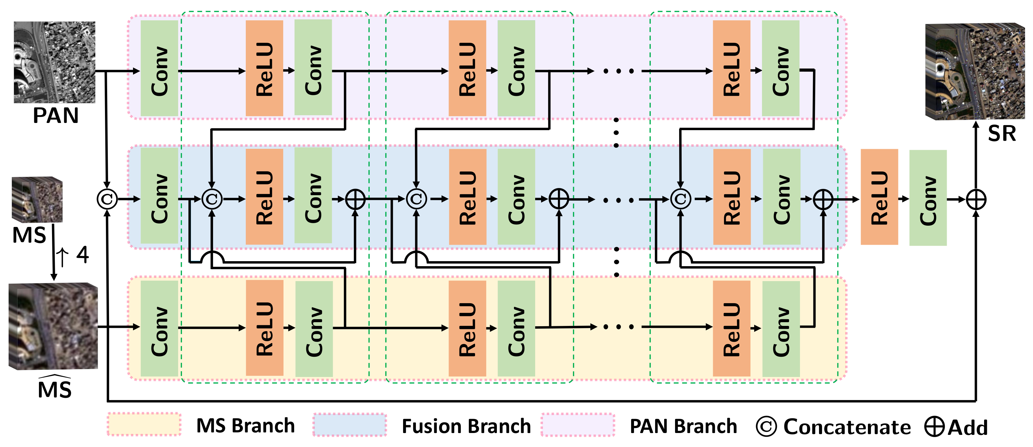
In this section, we will state the motivation of our work, and then introduce the details of the proposed FDFNet. Figure 2 shows the architecture of our proposed network.

3.1. Motivation

Although the methods mentioned above provided various empirical approaches to depict the relationships between images, three main limitations have not been addressed. First, they neglected the difference between the LR-MS image and HR-PAN images in terms of the spectral and spatial information, and were just fused through concatenation or summation at first, and then the fused image directly inputted into the network, leading to the features being separately contained in the HR-PAN image and LR-MS image, which cannot be effectively extracted. Second, the existing methods only perform feature fusion at the first or last layers in the network. Thus the resulting fusion image may be inadequate for discriminative representation and integration reasonably. Third, separate feature extraction and fusion operations will make the network structure complex and computationally expensive, resulting in a cumbersome model.

In response to the above concerns, we managed to extract the rich textures and details contained in the spatial domain of the PAN image and the spectral features contained in the MS image through two independent branches to maintain the integrity of the spectral information of the multispectral image and reduce the distortion of the spatial information. In order to reduce the computational burden of feature fusion, the features obtained from the PAN branch and MS branch at the same depth are injected into the fusion branch parallel to the other two branches. While performing feature extraction, the full-depth feature fusion of the network is realized. In this way, the network can maximize the use of features at different depths and branches, that is, low-level detailed texture features and high-level semantic features to restore distortion-free fusion images.

3.2. Parallel Full-Depth Feature Fusion Network

Consider a PAN image $\mathrm{PAN}\in {\mathbb{R}}^{\mathrm{H}\times \mathrm{W}\times 1}$ and a MS image $\mathrm{MS}\in {\mathbb{R}}^{\frac{\mathrm{H}}{4}\times \frac{\mathrm{W}}{4}\times \mathrm{b}}$, where b represents the number of band in the MS image. Firstly, $\mathrm{MS}$ will be upsampled to the same size as $\mathrm{PAN}$ by a polynomial kernel with 23 coefficients [76], and let $\widetilde{\mathrm{MS}}\in {\mathbb{R}}^{H\times W\times b}$ represent the upsampled image. Next, $\mathrm{PAN}$ and $\widetilde{\mathrm{MS}}$ will be concatenated together as an original fusion product $\mathrm{M}\in {\mathbb{R}}^{\mathrm{H}\times \mathrm{W}\times (\mathrm{b}+1)}$. Then, $\mathrm{PAN}$, $\widetilde{\mathrm{MS}}$, and $\mathrm{M}$ will be sent to three parallel convolutional layers respectively to increase the number of channels for later feature extraction.

The three feature maps, ${\mathrm{I}}_{\mathrm{pan}}$, ${\mathrm{I}}_{\mathrm{ms}}$, and ${\mathrm{I}}_{\mathrm{fuse}}$, obtained by the above operation will be fed into the head structure of three parallel branches. The three branches developed accordingly are called the PAN branch, MS branch, and fusion branch. Moreover, the features exacted from the PAN branch and MS branch will be injected into the fusion branch through the constructed parallel feature fusion block (PFFB). The details about PFFB can refer to Section 3.3 and Figure 3. In particular, there are 4 PFFBs contained in the proposed FDFNet.

The underlying detailed information and deep semantic information are fused through the distribution of PFFB in each depth of the network characteristics. We believe that such a full-depth fusion is beneficial to improving the network’s feature representation ability. After 4 PFFBs, the feature map from the fusion branch will be selected out and sent to a convolutional layer with beforehand ReLU activation to reduce its channels to the same as that of $\widetilde{\mathrm{MS}}$. The output feature is denoted as $\mathrm{S}\in {\mathbb{R}}^{\mathrm{H}\times \mathrm{W}\times \mathrm{b}}$. Finally, we add $\mathrm{S}$ and $\widetilde{\mathrm{MS}}$ that transferred by a long skip to yield the final super-resolution image $\mathrm{SR}\in {\mathbb{R}}^{\mathrm{H}\times \mathrm{W}\times \mathrm{b}}$. The whole process can be expressed as follows:

$$\mathrm{SR}={\mathcal{F}}_{\theta }([\widetilde{\mathrm{MS}};\mathrm{PAN}];\widetilde{\mathrm{MS}};\mathrm{PAN})+\widetilde{\mathrm{MS}},$$

(2)

where ${\mathcal{F}}_{\theta }(·)$ represents the FDFNet with its parameters $\theta$. For more details about FDFNet, refer to Figure 2.

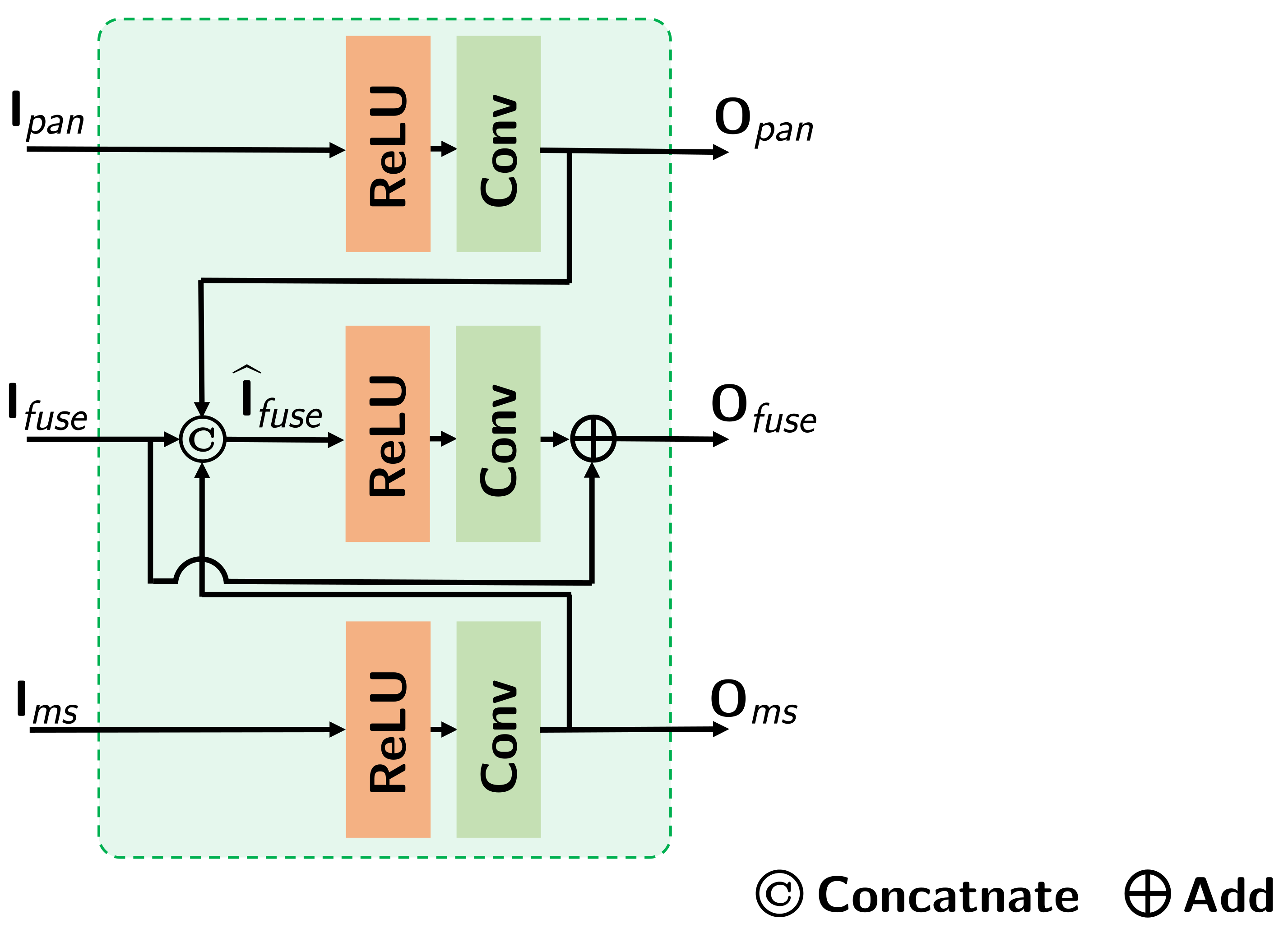
3.3. Parallel Feature Fusion Block

In order to realize the transfer and fusion of feature maps among the three branches, i.e., PAN branch, MS branch, and the fusion branch, we designed a parallel feature fusion block (PFFB). To facilitate the description, let ${\mathrm{I}}_{\mathrm{pan}}\in {\mathbb{R}}^{\mathrm{H}\times \mathrm{W}\times {\mathrm{C}}_{\mathrm{pan}}}$, ${\mathrm{I}}_{\mathrm{ms}}\in {\mathbb{R}}^{\mathrm{H}\times \mathrm{W}\times {\mathrm{C}}_{\mathrm{ms}}}$, and ${\mathrm{I}}_{\mathrm{fuse}}\in {\mathbb{R}}^{\mathrm{H}\times \mathrm{W}\times {\mathrm{C}}_{\mathrm{fuse}}}$, respectively, represent the input feature of PAN branch, the MS branch, and the fusion branch, while ${\mathrm{O}}_{\mathrm{pan}}\in {\mathbb{R}}^{\mathrm{H}\times \mathrm{W}\times {\mathrm{C}}_{\mathrm{pan}}}$, ${\mathrm{O}}_{\mathrm{ms}}\in {\mathbb{R}}^{\mathrm{H}\times \mathrm{W}\times {\mathrm{C}}_{\mathrm{ms}}}$, and ${\mathrm{O}}_{\mathrm{fuse}}\in {\mathbb{R}}^{\mathrm{H}\times \mathrm{W}\times {\mathrm{C}}_{\mathrm{fuse}}}$ represent output feature of PAN branch, the MS branch, and the fusion branch respectively, where H and W are the size in spatial dimension, and $C_{pan}$, $C_{ms}$, and $C_{fuse}$ denote the channels of the feature maps.

Firstly, ${\mathrm{I}}_{\mathrm{pan}}$ and ${\mathrm{I}}_{\mathrm{ms}}$ will be subjected to feature extraction operations and get their output features ${\mathrm{O}}_{\mathrm{pan}}$ and ${\mathrm{O}}_{\mathrm{ms}}$. After that, ${\mathrm{O}}_{\mathrm{pan}}$, ${\mathrm{O}}_{\mathrm{ms}}$, and ${\mathrm{I}}_{\mathrm{fuse}}$ will be concatenated together as ${\widehat{\mathrm{I}}}_{fuse}\in {\mathbb{R}}^{H\times W\times (C_{pan}+C_{ms}+C_{fuse})}$. The process can be expressed as follows:

$${\mathrm{O}}_{\mathrm{pan}}={\mathcal{C}}_{\mathrm{s}}\left(\mathcal{A}\left({\mathrm{I}}_{\mathrm{pan}}\right)\right);$$

(3)

$${\mathrm{O}}_{\mathrm{ms}}={\mathcal{C}}_{\mathrm{s}}\left(\mathcal{A}\left({\mathrm{I}}_{\mathrm{ms}}\right)\right);$$

(4)

$${\widehat{\mathrm{I}}}_{fuse}=[{\mathrm{O}}_{\mathrm{pan}};{\mathrm{O}}_{\mathrm{ms}};{\mathrm{I}}_{\mathrm{fuse}}],$$

(5)

where ${\mathcal{C}}_s(·)$ and $\mathcal{A}(·)$ represents the convolutional layer in which the input channel is the same as the output channel, and $\mathcal{A}(·)$ represents ReLU activation. Finally, ${\widehat{\mathrm{I}}}_{fuse}$ will be subjected to feature extraction operation and added with ${\mathrm{I}}_{\mathrm{fuse}}$ by a short connection as the output feature ${\mathrm{O}}_{\mathrm{fuse}}$. The final process in PFFB can be expressed as follows:

$${\mathrm{O}}_{\mathrm{fuse}}={\mathcal{C}}_{\mathrm{r}}\left(\mathcal{A}\left({\widehat{\mathrm{I}}}_{\mathrm{fuse}}\right)\right)+{\mathrm{I}}_{\mathrm{fuse}},$$

(6)

where ${\mathcal{C}}_r(·)$ represents the convolutional layer which will reduce the channels of the exacted feature to the same as ${\mathrm{I}}_{\mathrm{fuse}}$. For more details about PFFB, refer to Figure 3.

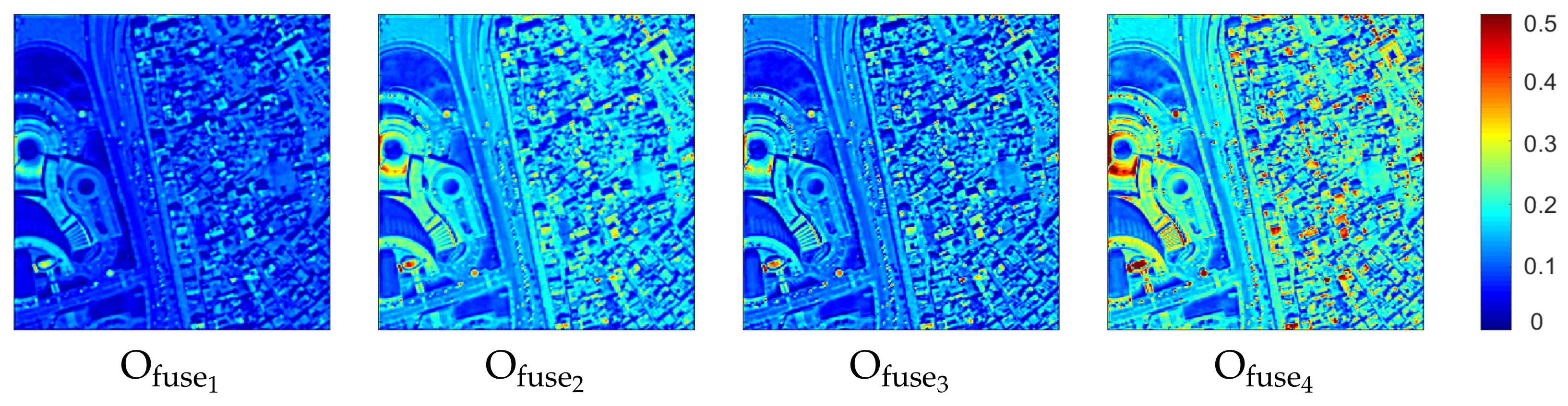
We show the output of 4 PFFBs, i.e., ${\mathrm{O}}_{{\mathrm{fuse}}_{\mathrm{i}}},i=1,\dots ,4$ in Figure 4. It can be seen that as the depth becomes deeper, more and more details are perceived. The contours of buildings and streets are also more clearly portrayed, ultimately in the form of high-frequency information. Compared with the previous three images, the last feature map ${\mathrm{O}}_{{\mathrm{fuse}}_4}$ shows a greater difference between its maximum and minimum values. More sporadic red portions imply more chromatic aberration, sharper edge outlines, and high-frequency information, all of which are in line with our expectations.

The closer to the bottom layer, the more blurred our information and the smaller the targets that can be detected, as the ${\mathrm{O}}_{{\mathrm{fuse}}_1}$ shows in Figure 4, which is also indispensable. To get in-depth high-frequency information while retaining shallow information simultaneously, we try to skip connections between neighboring PFFB modules. By leveraging on the skip connection, the product of the previous block can be transferred to the deep layers, which retains the shallow features and enriches the deep semantics.

3.4. Loss Function

To depict the difference between SR and the ground-truth (GT) image, we adopt the mean square error (MSE) to optimize the proposed framework in the training process. The loss function can be expressed as follows:

$$\mathcal{L}\left(\theta \right)=\frac{1}{N}\sum _{i=1}^N∥{\mathcal{F}}_{\theta }([{\widetilde{\mathrm{MS}}}^{\left(i\right)};{\mathrm{PAN}}^{\left(\mathrm{i}\right)}];{\widetilde{\mathrm{MS}}}^{\left(\mathrm{i}\right)};{\mathrm{PAN}}^{\left(\mathrm{i}\right)})+{{\widetilde{\mathrm{MS}}}^{\left(i\right)}-{\mathrm{GT}}^{\left(\mathrm{i}\right)}∥}_F^2,$$

(7)

where N represents the number of training samples, and ${∥·∥}_F$ is the Frobenius Norm.

4. Experiments

This section is for experimental evaluation. The proposed FDFNet is compared with some recent competitive approaches on various datasets obtained by WorldView-3 (WV3), QuickBird (QB), and GaoFen-2 (GF2) satellites. First, the preprocessing of the dataset and the training details will be described. Then, the quantitative metrics and visual results on reduced-resolution and full-resolution will be presented to illustrate the effectiveness of the full-depth feature fusion scheme. Finally, extensive ablation studies analyze how the proposed full-depth fusion scheme benefits the fusion process. Moreover, once our paper is accepted, the source code of training and testing will be open-sourced.

4.1. Dataset

To benchmark the effectiveness of FDFNet for pansharpening, we adopted a wide range of datasets, including 4-band datasets captured by QuickBird (QB) and GaoFen-2 (GF2) satellites and 8-band datasets captured by WorldView-3 (WV3). The former 4-band dataset contains four standard colors (red, green, blue, and near-infrared). Based on these, the 8-band dataset adds four new bands (coastal, yellow, red edge, and near-infrared). The spatial resolution ratio between PAN and MS is equal to 4. As the ground truth (GT) images are not available, Wald’s protocol [77] is performed to ensure the baseline image generation. In particular, the steps for generating the training and testing data for performance assessment are as follows: (1) Downsample the original HR-PAN and LR-MS image by a downsampling factor 4 through satellite corresponding modulation transfer function (MTF) based filters; (2) take the downsampled HR-PAN image as the simulated PAN image and the downsampled LR-MS image as the simulated LR-MS image; and (3) take the original MS image as the simulated GT image. The specific information of different simulated dataset are listed as follows:

• For WV3 data, we downloaded the datasets from the public website (http://www.digitalglobe.com/samples?search=Imagery, accessed on 6 April 2021) and obtained 12,580 PAN/MS/GT image pairs ($70\%$/$20\%$/$10\%$ as training/validation/testing dataset) with a size of 64 × 64 × 1, 16 × 16 × 8, and 64 × 64 × 8, respectively, the resolution of PAN and MS are 0.5 m and 2 m per pixel. For testing, we used not only the 1258 small patches mentioned above, but also the large patches of a new WorldView-3 dataset that captured Rio’s scenarios (size: $256\times 256\times 4$);
• For QB data, we downloaded a large dataset ($4906\times 4906\times 4$) acquired over the city of Indianapolis and cut it into two parts. The left part ($4906\times 2906\times 4$) is used to simulate 20,685 training PAN/MS/GT image pairs with the size 64 × 64 × 1, 16 × 16 × 4, and 64 × 64 × 4, respectively, the resolution of PAN and MS are 0.61 m and 2.4 m per pixel, and the right part ($4906\times 1000\times 4$) is used to simulate 48 testing data (size: $256\times 256\times 4$);
• For GF2 data, we downloaded a large dataset ($6907\times 7300\times 4$) over the city of Beijing from the website (http://www.rscloudmart.com/dataProduct/sample, accessed on 6 April 2021) to simulate 21,607 training PAN/MS/GT image pairs with the size 64 × 64 × 1, 16 × 16 × 4, and 64 × 64 × 4, the resolution of PAN and MS are 0.8 m and 3.2 m per pixel. Besides, a huge image acquired over the cit of Guangzhou was downloaded to simulate 81 testing data (size: $256\times 256\times 4$).

It is worth mentioning that our patches all come from a single acquisition and there is no network generalization problem.

4.2. Training Details and Parameters

Due to the different number of bands, we make separate training and test datasets on WV3, QB, and GF2, as described in Section 4.1, train the network, and test separately on each dataset. All DL-based methods are fairly trained on the same dataset on NVIDIA GeForce GTX 2080Ti with 11 GB. Besides, we set 1000 epochs for the FDFNet training under the Pytorch framework, while the learning rate is set to $3\times {10}^{-4}$ for the first 500 epochs and $1\times {10}^{-4}$ for the last 500 epochs, which is set and adjusted empirically according to the loss curve during training. $C_{pan}$ and $C_{ms}$ are set as 16, $C_{fuse}$ is set as 32, and four PFFBs are included in the network. We employed Adam [78] as the optimizer to optimize the parameters, with batch size 32 while ${\beta }_1$ and ${\beta }_2$ are set as 0.9 and 0.999, respectively. The batch size has little effect on the final result. As for betta1 and 2, both are the default settings for the optimizer Adam, and we achieved satisfactory results without adjusting them. We use the source codes provided by the authors or re-implement the code with the default parameters in the corresponding papers for the compared approaches.

4.3. Comparison Methods and Quantitative Metrics

For comparison, we select 10 state-of-the-art traditional fusion mathods based on CS/MRA, including EXP [76], GS [5], CNMF [79], HPM [10], GLP-CBD [1], GLP-Reg [36], BDSD-PC [3], BDSD [2], PRACS [4], and SFIM [6]. Two VO-based methods are also added to the list of competitors, including DGS [13] and LGC(CVPR19) [12]. In addition, six recently widely-accepted proposed deep convolutional networks for pan-sharpening are used to compare the performance of the trained model, including PNN [37], PanNet [35], DiCNN1 [36], LPPN [42], BDPN [41], and DMDNet [34].

Quality evaluation is carried out at reduced and full resolutions. For the reduced-resolution test, the relative dimensionless global error in synthesis (ERGAS) [80], the spectral angle mapper (SAM) [81], the spatial correlation coefficient (SCC) [82], and quality index for 4-band images (Q4) or 8-band images (Q8) [83] are used to assess the quality of the results. In addition, to evaluate the performance of all involved methods on full-resolution, the QNR, $D_{\lambda }$, and $D_s$ [84,85] indexes are applied.

4.4. Performance Comparison with Reduced-Resolution WV3 Data

We compare the performance of all the introduced benchmarks on the 1258 testing samples. For each testing example, the sizes of PAN, MS, and GT images are the same as that of the training examples, i.e., 64 × 64 for the PAN image, $16\times 16\times 8$ for the original low spatial resolution MS image, and $64\times 64\times 8$ for the GT image.

Table 1. Average quantitative with the related standard deviations (std) comparisons on 1258 reduced-resolution WV3 examples. The best performance is shown in bold and second place is underlined.

Method	SAM	ERGAS	SCC	Q8
EXP [76]	5.8531 ± 1.9931	7.0446 ± 2.9339	0.6604 ± 0.1062	0.6267 ± 0.1418
GS [5]	5.6982 ± 2.0077	5.2817 ± 2.1867	0.8725 ± 0.0705	0.7655 ± 0.1394
CNMF [79]	5.5310 ± 1.8756	4.6183 ± 1.9297	0.8877 ± 0.0680	0.8216 ± 0.1229
MTF-GLP-HPM [10]	5.6035 ± 1.9739	4.7638 ± 1.9345	0.8729 ± 0.0650	0.8171 ± 0.1279
MTF-GLP-CBD [1]	5.2861 ± 1.9582	4.1627 ± 1.7748	0.8904 ± 0.0698	0.8540 ± 0.1144
MTF-GLP-Reg [11]	5.2602 ± 1.9426	4.1571 ± 1.7748	0.8914 ± 0.0690	0.8536 ± 0.1148
BDSD-PC [3]	5.4251 ± 1.9716	4.2460 ± 1.8602	0.8913 ± 0.0704	0.8528 ± 0.1164
BDSD [2]	6.9997 ± 2.8530	5.1670 ± 2.2475	0.8712 ± 0.0798	0.8126 ± 0.1234
PRACS [4]	5.5885 ± 1.9811	4.6896 ± 1.8535	0.8657 ± 0.0808	0.8132 ± 0.1295
SFIM [6]	5.4519 ± 1.9025	5.1995 ± 6.5738	0.8663 ± 0.0670	0.7979 ± 0.1220
DGS [13]	6.5096 ± 1.7344	5.3098 ± 1.5556	0.8647 ± 0.0656	0.8035 ± 0.1333
LGC [12]	5.2102 ± 1.8703	5.1402 ± 2.1209	0.8670 ± 0.6040	0.7930 ± 0.1232
PNN [37]	4.0015 ± 1.3292	2.7283 ± 1.0042	0.9515 ± 0.0465	0.9083 ± 0.1122
PanNet [35]	4.0921 ± 1.2733	2.9524 ± 0.9778	0.9495 ± 0.0461	0.8942 ± 0.1170
DiCNN1 [36]	3.9805 ± 1.3181	2.7367 ± 1.0156	0.9517 ± 0.0472	0.9097 ± 0.1117
LPPN [42]	3.9021 ± 1.2901	2.6404 ± 0.9600	0.9552 ± 0.0450	0.9130 ± 0.1110
BDPN [41]	3.9952 ± 1.3869	2.7234 ± 1.0394	0.9515 ± 0.0457	0.9123 ± 0.1128
DMDNet [34]	3.9714 ± 1.2482	2.8572 ± 0.9663	0.9527 ± 0.0447	0.9000 ± 0.1142
FDFNet	3.6584 ± 1.2252	2.5109 ± 0.9423	0.9597 ± 0.0445	0.9171 ± 0.1107
Ideal value	0	0	1	1

reports the average and standard deviation metrics of all compared methods. It is clear that the proposed FDFNet outperforms other advanced methods in terms of all the assessment metrics. Specifically, the result obtained by our network exceeds the average value of DMDNet in SAM and ERGAS by almost 0.3, which is a noticeable improvement. Since SAM and ERGAS are the measures for spectral and spatial fidelity, respectively, it is easy to know that FDFNet can strike a satisfying balance between spectral and spatial information.

In addition, it can be seen that DL-based methods outperform traditional CS/MRA methods, but on the other hand, this superiority is based on large-scale training data. Therefore, we also introduce a new WorldView-3 dataset that captured Rio’s scenarios, which never fed into the networks in their training phase. The Rio dataset holds 30-cm resolution, and the size of the GT, HR-PAN, and LR-MS image is 256 × 256 × 8, 256 × 256, and 64 × 64 × 8, respectively. Then, we test all the methods on the Rio dataset, and the results are shown in

Table 2. Average quantitative comparisons on the Rio dataset. The best performance is shown in bold and second place is underlined.

Method	SAM	ERGAS	SCC	Q8	Time
EXP [76]	7.0033	6.5368	0.6927	0.6156	0.0312
GS [5]	8.9481	6.3662	0.6775	0.8666	0.0440
CNMF [79]	7.1099	4.9868	0.7617	0.7576	0.0328
MTF-GLP-HPM [10]	7.2994	5.1185	0.7369	0.7849	0.2037
MTF-GLP-CBD [1]	7.4053	5.0372	0.6738	0.7880	0.1069
MTF-GLP-Reg [11]	7.3275	5.0154	0.6822	0.7889	0.1476
BDSD-PC [3]	7.0721	4.9515	0.7164	0.7853	0.1701
BDSD [2]	7.1218	4.9413	0.7186	0.7787	0.0796
PRACS [4]	7.1176	5.5392	0.6370	0.7380	0.1765
SFIM [6]	6.8501	4.9571	0.7558	0.7882	0.0251
DGS [13]	7.8368	5.6175	0.6861	0.6542	0.9723
LGC [12]	6.3115	5.1177	0.7715	0.7356	1.3278
PNN [37]	4.0659	2.7144	0.9487	0.8888	0.5475
PanNet [35]	3.9062	2.6583	0.9522	0.8814	0.5880
DiCNN1 [36]	3.8289	2.5819	0.9544	0.8895	0.5527
LPPN [42]	3.7118	2.4882	0.9591	0.8976	0.4987
BDPN [41]	4.0788	2.6897	0.9439	0.8969	0.8796
DMDNet [34]	3.6917	2.4968	0.9594	0.8990	0.6198
FDFNet	3.3801	2.3522	0.9649	0.9155	0.5019
Ideal value	0	0	1	1

. Consistent with previous results, our method performs best on all indicators.

Moreover, we compare the testing time of all methods on the Rio dataset to prove its efficiency. The recording is reported in the last column of Table 2. It is obvious that FDFNet takes the shortest time compared to other DL-based methods, reflecting the high efficiency of full-depth integration and parallel working.

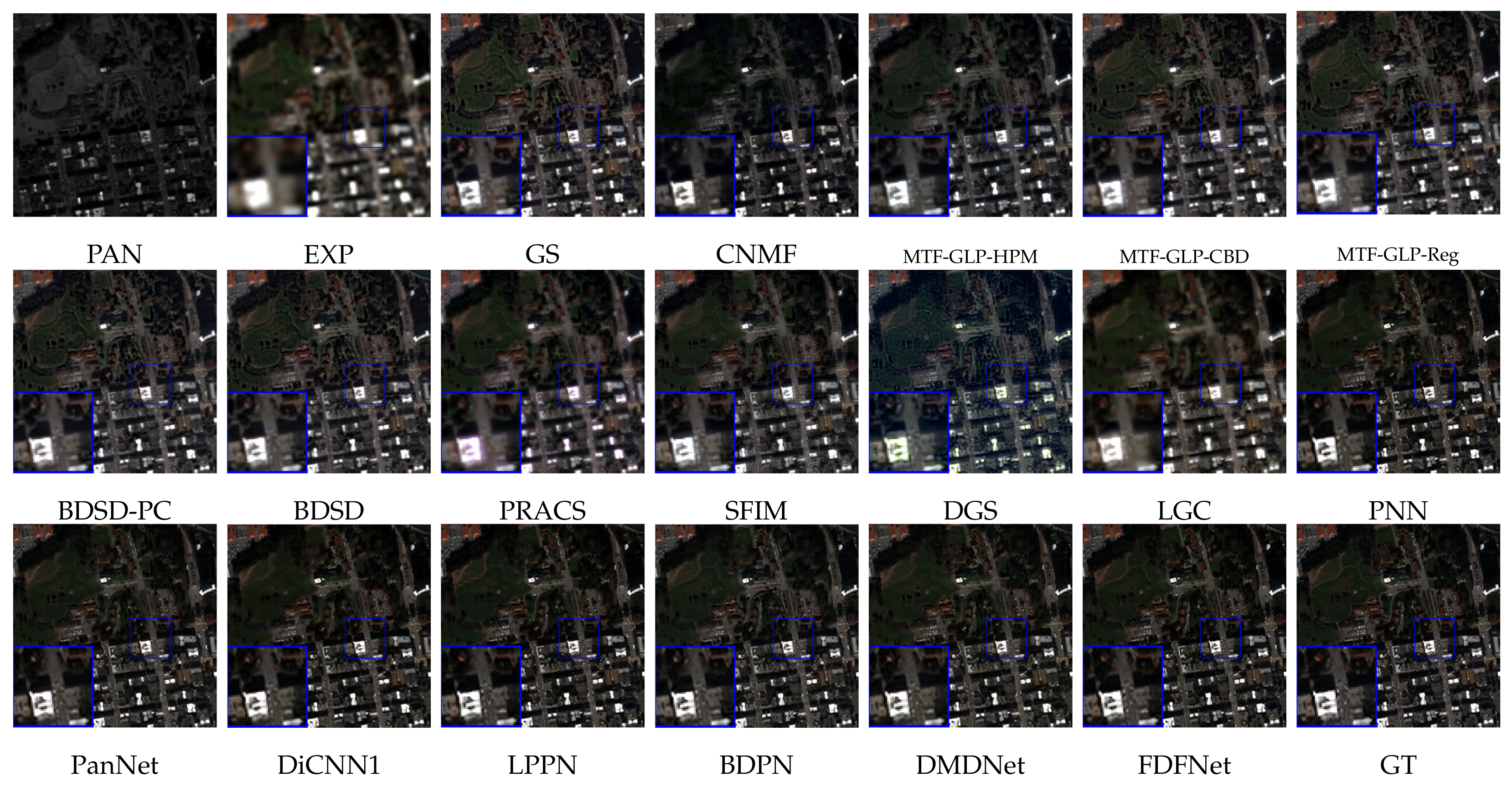
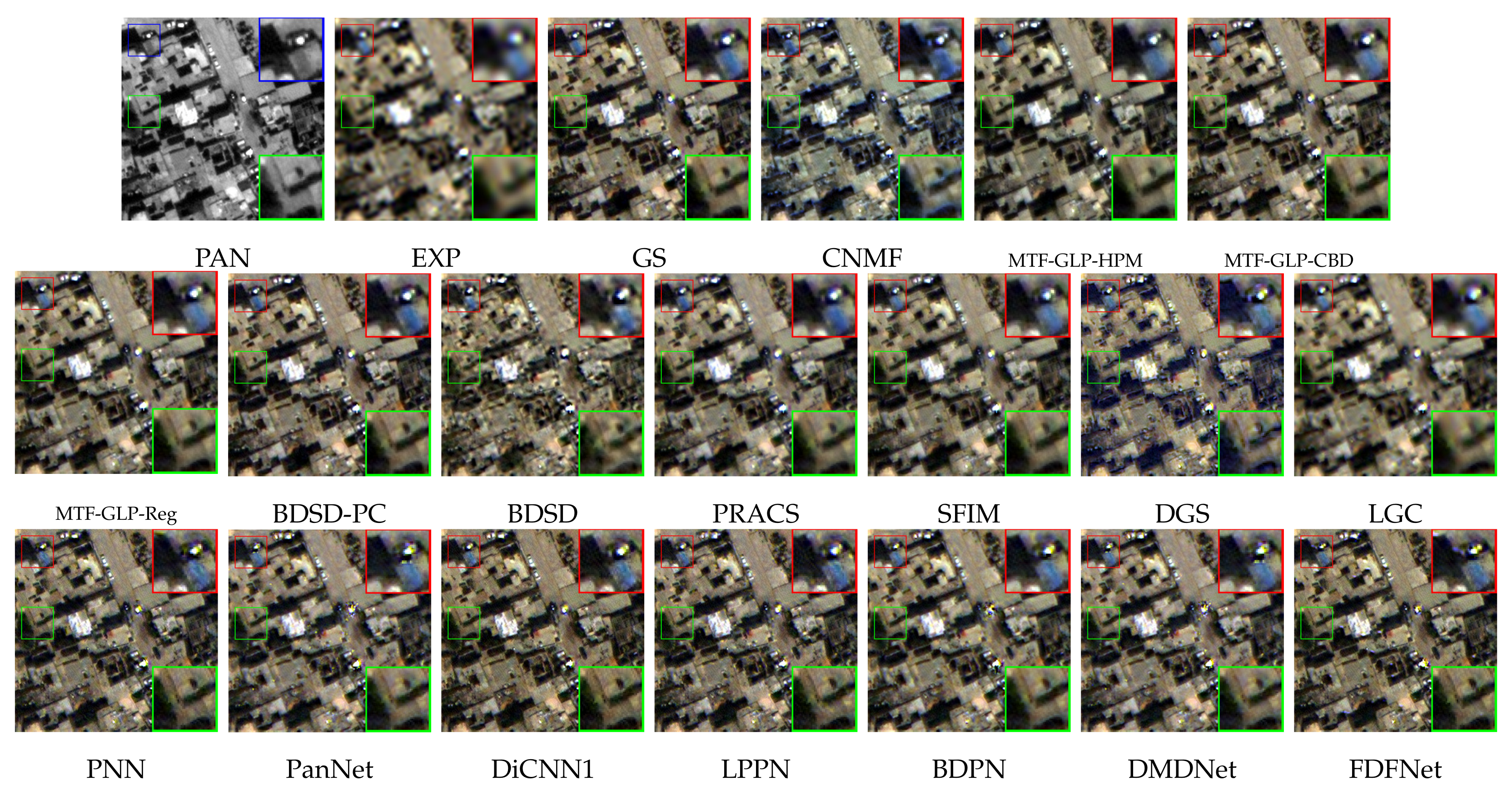
We also display a visual comparison of our FDFNet with other state-of-the-art methods, as shown in Figure 5. To facilitate the distinction between the quality of the results, we also show the corresponding residual map in Figure 6, which takes the GT image as a reference. The FDFNet yields more details with less blurring, especially in areas with dense buildings. These results verify that FDFNet indeed exploits the rich texture from the source images. Compared with other methods, FDFNet performs feature fusion at all depths, which covers the detailed features of the shallow layer and the semantic features of the deep layer. It is worth noting that in this case, LPPN and DMDNet are not so far from the proposal.

4.5. Performance Comparison with Reduced-Resolution 4-Band Data

We also assess the proposed method on 4-band datasets, including QB and GF2 data. The quantitative results in terms of all indicators are reported in

Table 3. Average quantitative with the related standard deviations (std) comparisons on 48 reduced-resolution QB examples. The best performance is shown in bold and second place is underlined.

Method	SAM	ERGAS	SCC	Q4
EXP [76]	8.1569 ± 1.9571	11.5679 ± 2.1892	0.5242 ± 0.0223	0.5728 ± 0.1064
GS [5]	8.1899 ± 1.9738	9.2075 ± 1.5195	0.8409 ± 0.0632	0.7192 ± 0.1093
CNMF [79]	7.3469 ± 2.3535	7.8355 ± 1.1998	0.8233 ± 0.2183	0.7438 ± 0.2117
MTF-GLP-HPM [10]	7.8945 ± 1.9769	8.0556 ± 1.1504	0.8389 ± 0.0605	0.7847 ± 0.1207
MTF-GLP-CBD [1]	7.3983 ± 1.7826	7.2965 ± 0.9316	0.8543 ± 0.0643	0.8191 ± 0.1283
MTF-GLP-Reg [11]	7.3848 ± 1.7796	7.3005 ± 0.9352	0.8549 ± 0.0640	0.8184 ± 0.1282
BDSD-PC [3]	7.6593 ± 1.9012	7.4584 ± 0.9910	0.8512 ± 0.0622	0.8139 ± 0.1365
BDSD [2]	7.6708 ± 1.9110	7.4661 ± 0.9912	0.8512 ± 0.0622	0.8132 ± 0.1361
PRACS [4]	7.8343 ± 1.9136	8.2135 ± 1.0862	0.8315 ± 0.0921	0.7730 ± 0.1416
SFIM [6]	7.7175 ± 1.8718	8.7782 ± 2.3796	0.8321 ± 0.1054	0.7670 ± 0.1362
DGS [13]	8.2770 ± 1.8213	8.4872 ± 1.2444	0.8264 ± 0.0534	0.7725 ± 0.1199
LGC [12]	7.6957 ± 1.8428	9.1597 ± 1.5275	0.8215 ± 0.0459	0.7234 ± 0.1292
PNN [37]	5.1993 ± 0.9474	4.8712 ± 0.4584	0.9324 ± 0.0489	0.8872 ± 0.1481
PanNet [35]	5.3144 ± 1.0175	5.1623 ± 0.6815	0.9296 ± 0.0586	0.8834 ± 0.1399
DiCNN1 [36]	5.3071 ± 0.9958	5.2310 ± 0.5412	0.9224 ± 0.0507	0.8821 ± 0.1432
LPPN [42]	5.0133 ± 0.9753	5.1500 ± 1.0914	0.9410 ± 0.0483	0.8851 ± 0.1379
BDPN [41]	5.7145 ± 1.1475	5.0497 ± 0.5370	0.9242 ± 0.0477	0.8854 ±0.1411
DMDNet [34]	5.1197 ± 0.9399	4.7377 ± 0.6487	0.9350 ± 0.0653	0.8908 ± 0.1464
FDFNet	4.7924 ± 0.8397	4.3020 ± 0.2797	0.9463 ± 0.0469	0.9032 ± 0.1392
Ideal value	0	0	1	1

and

Table 4. Average quantitative with the related standard deviations (std) comparisons on 81 reduced-resolution GF2 examples. The best performance is shown in bold and second place is underlined.

Method	SAM	ERGAS	SCC	Q4
EXP [76]	2.4687 ± 0.5213	2.8812 ± 0.8481	0.7305 ± 0.0742	0.7793 ± 0.0466
GS [5]	2.9751 ± 1.1114	2.9661 ± 1.0105	0.8523 ± 0.0618	0.7865 ± 0.0759
CNMF [79]	2.4961 ± 0.7159	2.2094 ± 0.6601	0.8787 ± 0.0522	0.8426 ± 0.0478
MTF-GLP-HPM [10]	2.5522 ± 0.7773	2.2994 ± 0.7128	0.8670 ± 0.0537	0.8522 ± 0.0451
MTF-GLP-CBD [1]	2.2744 ± 0.7335	2.0461 ± 0.6198	0.8728 ± 0.0527	0.8773 ± 0.0406
MTF-GLP-Reg [11]	2.2528 ± 0.7124	2.0251 ± 0.6050	0.8745 ± 0.0516	0.8786 ± 0.0394
BDSD-PC [3]	2.3042 ± 0.6432	2.0752 ± 0.6040	0.8776 ± 0.0511	0.8780 ± 0.0404
BDSD [2]	2.3074 ± 0.6693	2.0704 ± 0.6097	0.8769 ± 0.0516	0.8763 ± 0.0417
PRACS [4]	2.3113 ± 0.5970	2.1685 ± 0.5992	0.8666 ± 0.0497	0.8719 ± 0.0347
SFIM [6]	2.2970 ± 0.6378	2.1887 ± 0.6950	0.8608 ± 0.0541	0.8651 ± 0.0403
DGS [13]	2.5133 ± 0.4293	2.5719 ± 0.4791	0.8159 ± 0.0440	0.7795 ± 0.0840
LGC [12]	2.1582 ± 0.5011	2.2495 ± 0.6433	0.8708 ± 0.0411	0.8661 ± 0.0278
PNN [37]	1.4599 ± 0.3607	1.2707 ± 0.3243	0.9481 ± 0.0207	0.9474 ± 0.0203
PanNet [35]	1.3954 ± 0.3262	1.2239 ± 0.2828	0.9558 ± 0.0123	0.9469 ± 0.0222
DiCNN1 [36]	1.4948 ± 0.3814	1.3203 ± 0.3544	0.9459 ± 0.0223	0.9445 ± 0.0212
LPPN [42]	1.3408 ± 0.2559	1.1236 ± 0.2236	0.9609 ± 0.0085	0.9515 ± 0.0219
BDPN [41]	1.4876 ± 0.3861	1.2988 ± 0.3464	0.9301 ± 0.0207	0.9267 ±0.0212
DMDNet [34]	1.2968 ± 0.3156	1.1281 ± 0.2670	0.9645 ± 0.0101	0.9530 ± 0.0219
FDFNet	1.2772 ± 0.3035	1.0963 ± 0.2681	0.9638 ± 0.0104	0.9593 ± 0.0170
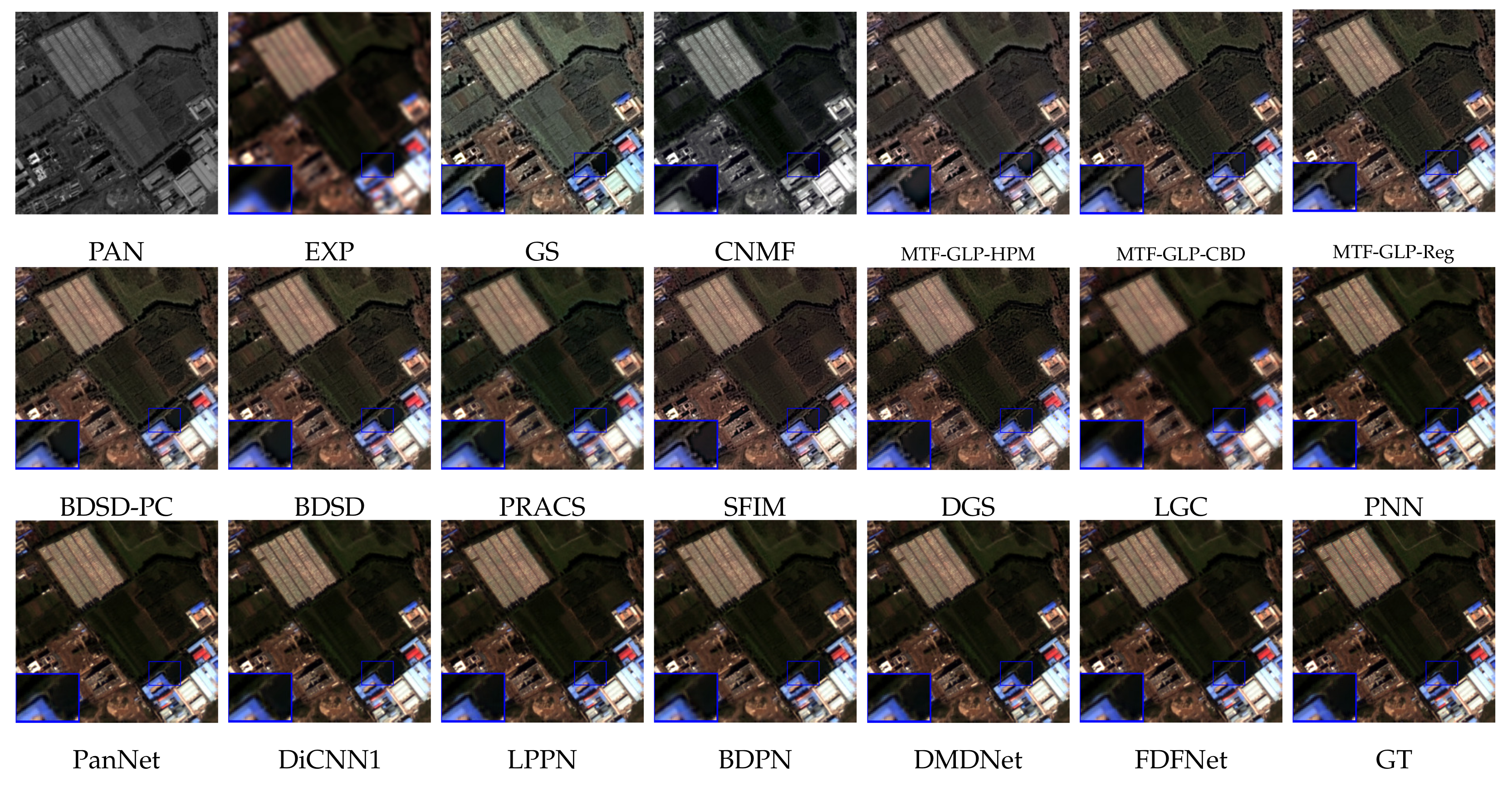
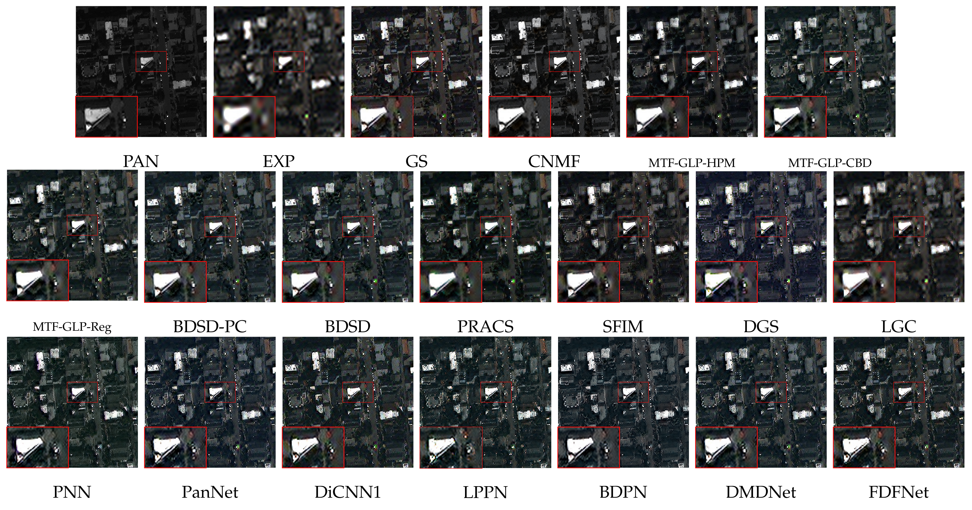
Ideal value	0	0	1	1

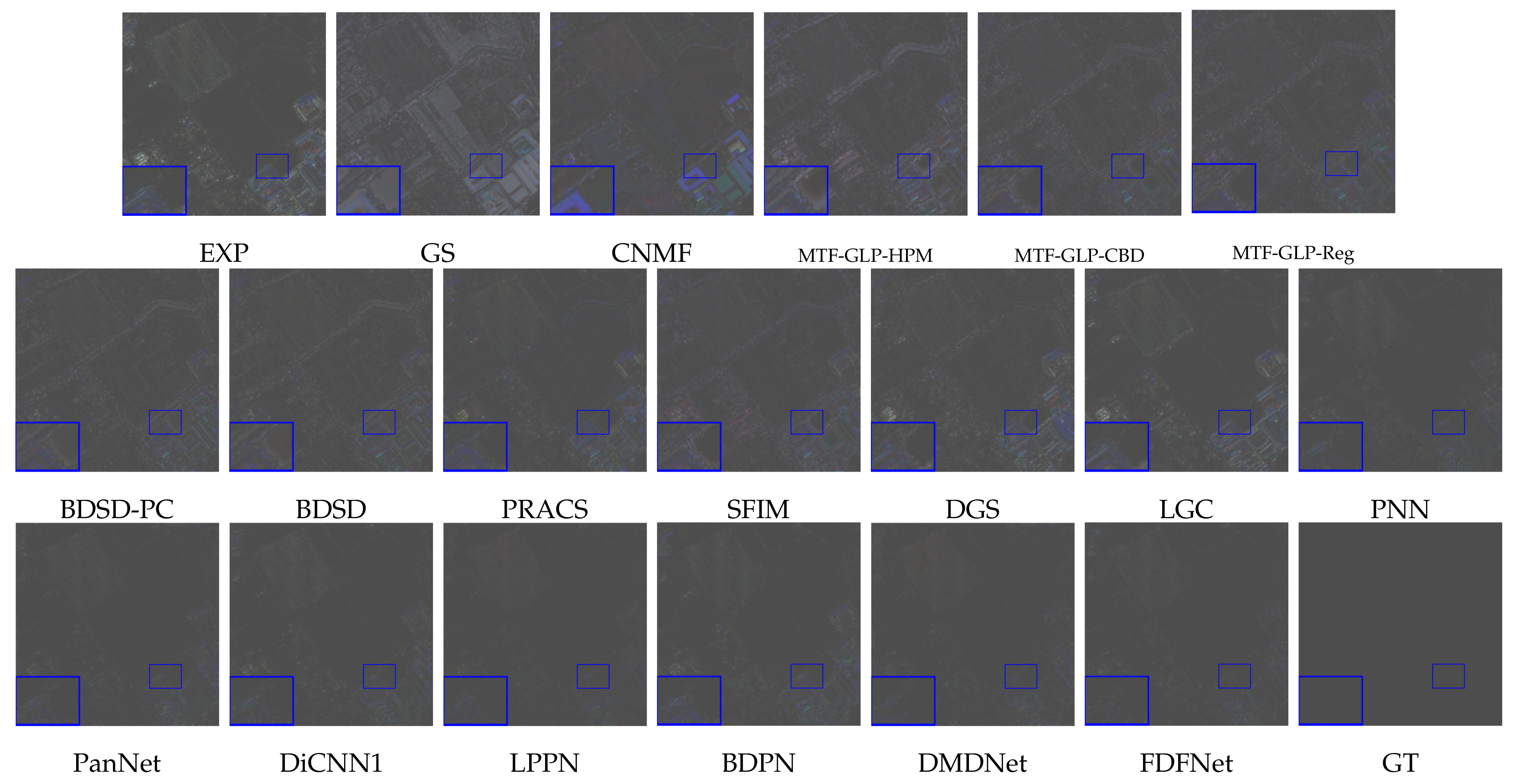
. As can be seen, the proposed method outperforms other competing methods with lower SAM and ERGAS and higher Q8 and SCC, which proves that the proposed framework can tackle with 4-band data effectively. We can see visual results from Figure 7 and Figure 8. Whether the images are recorded on sea or land, the fusion results of DFDNet are the closest to those of GT images, without noticeable artifacts or spectral distortions. This is more evident from the residual maps showed in Figure 9 and Figure 10, where the FDFNet produces more visually appealing results with less residual.

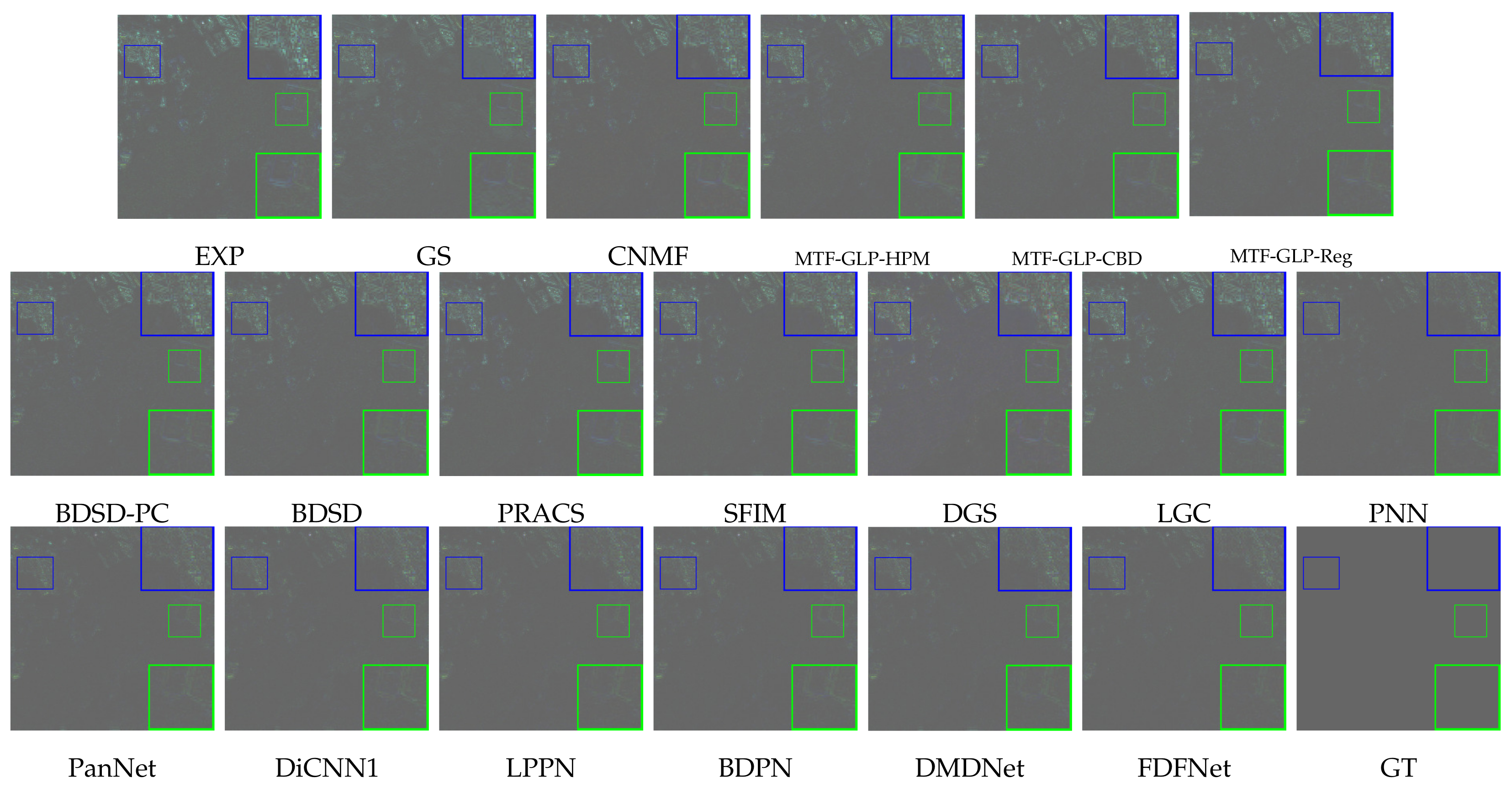
4.6. Performance Comparison with Full-Resolution WV3 Data

In this section, we assess the proposed framework on full-resolution data to test its performance on real data, since the various methods of pansharpening are ultimately applied in the actual scene without the reference images. Similarly to the experiments on reduced-resolution, both the quantitative and visual comparison are operated.

The results of quantitative experiments can refer to

Table 5. The average quantification compared to the relative standard deviation (std) of 50 full-resolution WV3 samples. The best performance is shown in bold and second place is underlined.

Method	QNR	${\mathit{D}}_{\mathit{\lambda }}$	${\mathit{D}}_{\mathit{s}}$
EXP [76]	0.2383 ± 0.3993	-/-	0.0259 ± 0.0486
GS [5]	0.8883 ± 0.0754	0.0231 ± 0.0325	0.0922 ± 0.0531
CNMF [79]	0.8682 ± 0.1093	0.0561 ± 0.0557	0.0841 ± 0.0732
MTF-GLP-HPM [1]	0.8902 ± 0.3892	0.0154 ± 0.0358	0.0198 ± 0.0444
MTF-GLP-CBD [1]	0.9001 ± 0.0813	0.0370 ± 0.0397	0.0672 ± 0.0522
MTF-GLP-Reg [11]	0.9014 ± 0.0783	0.0362 ± 0.0383	0.0664 ± 0.0499
BDSD-PC [3]	0.8991 ± 0.0802	0.0275 ± 0.0310	0.0770 ± 0.0578
BDSD [2]	0.9193 ± 0.0645	0.0220 ± 0.0195	0.0608 ± 0.0510
PRACS [4]	0.8959 ± 0.0736	0.0249 ± 0.0279	0.0825 ± 0.0542
SFIM [6]	0.9210 ± 0.0626	0.0296 ± 0.0341	0.0520 ± 0.0037
DGS [13]	0.9195 ± 0.0734	0.0446 ± 0.0470	0.0392 ± 0.0377
LGC [12]	0.9231 ± 0.0334	0.0188 ± 0.0171	0.0629 ± 0.0281
PNN [37]	0.9532 ± 0.0405	0.0216 ± 0.0223	0.0260 ± 0.0219
PanNet [35]	0.9516 ± 0.0298	0.0270 ± 0.0149	0.0221 ± 0.0171
DiCNN1 [36]	0.9383 ± 0.0562	0.0217 ± 0.0263	0.0416 ± 0.0355
LPPN [42]	0.9536 ± 0.0322	0.0241 ± 0.0174	0.0226 ± 0.0224
BDPN [41]	0.9532 ± 0.0405	0.0216 ± 0.0223	0.0260 ± 0.0219
DMDNet [34]	0.9539 ± 0.0268	0.0226 ± 0.0121	0.0241 ± 0.0174
FDFNet	0.9542 ± 0.0366	0.0150 ± 0.0080	0.0282 ± 0.0180
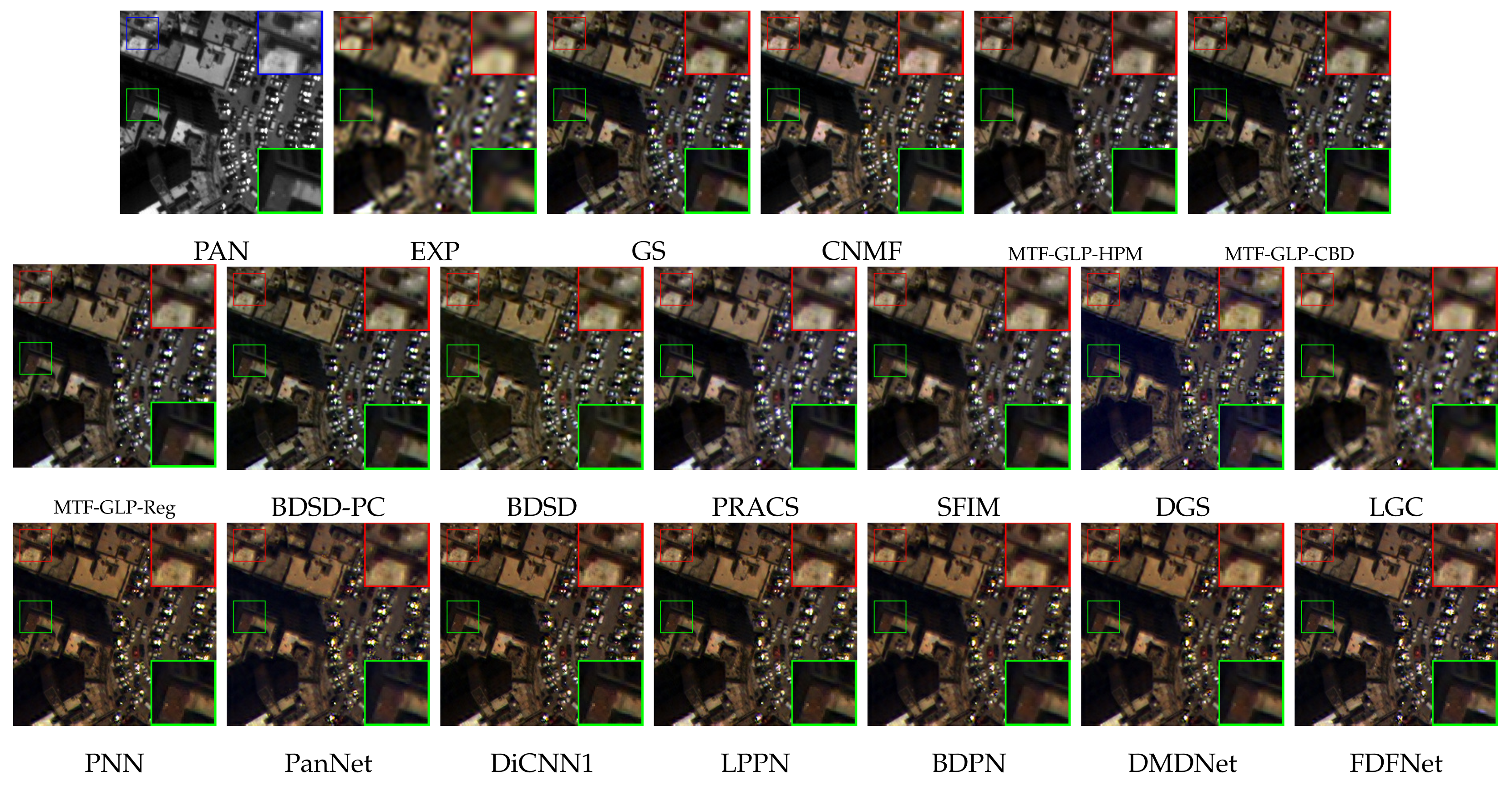
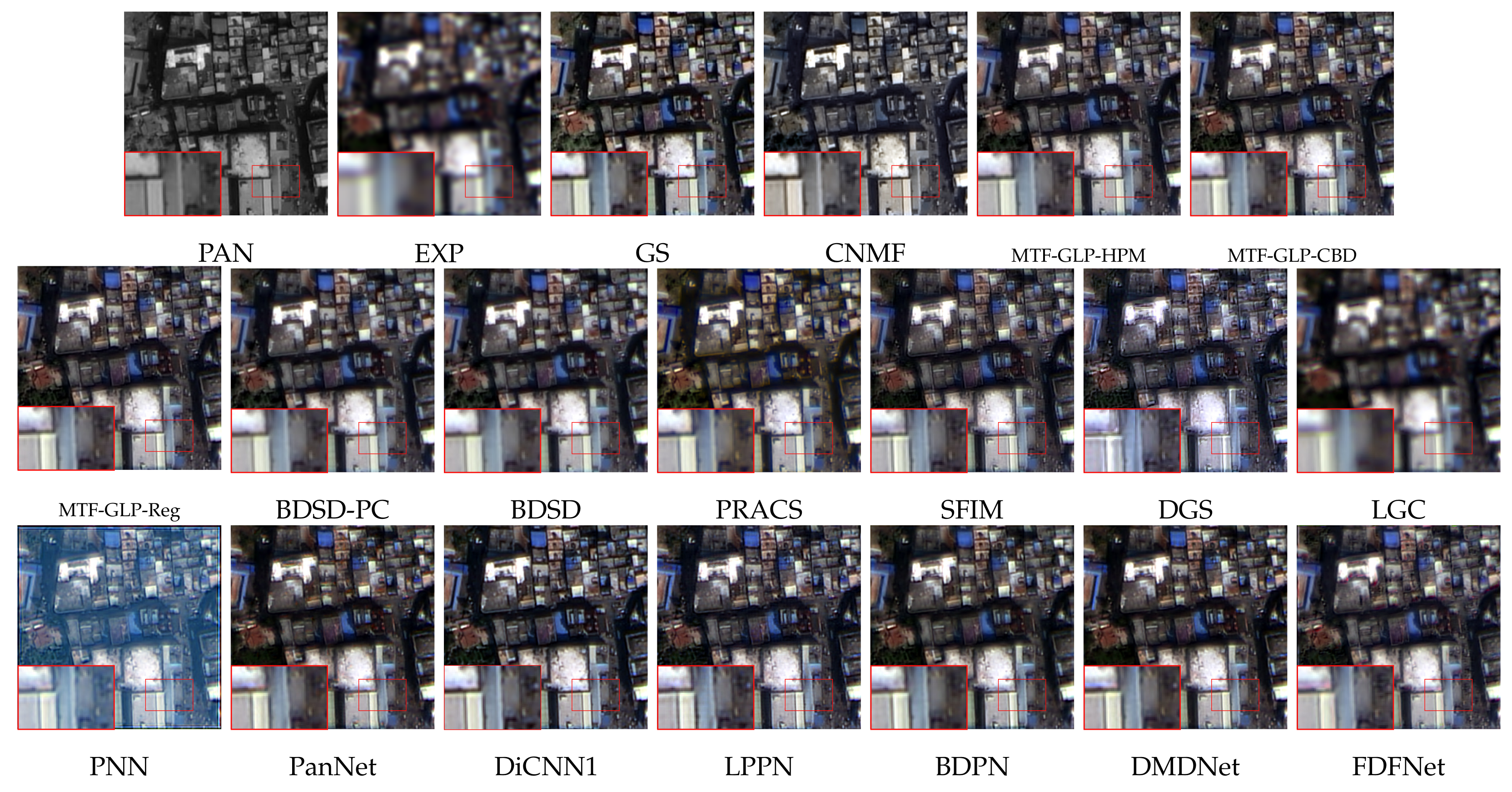
Ideal value	1	0	0

. The proposed FDFNet has achieved optimal or suboptimal results on several indicators. It is worth noting that although some DL-based methods perform well in reduced-resolution, some indicators are even inferior to some traditional techniques in full-resolution, which also verifies the importance of network generalization. Furthermore, through the visual experiment of Figure 11 and Figure 12, the pros and cons of various methods can be more intuitively reflected. Obviously, the super-resolution MS image texture obtained by our method is clearer, and there are no artifacts as DMDNet and PANNet yield. This also demonstrates that FDFNet has good generalization capabilities and can deal with pansharpening problems in actual application scenarios more effectively.

4.7. Performance Comparison with Full-Resolution 4-Band Data

We also compare the proposed method on 4-band full-resolution datasets, including QB and GF2 data. The quantitative results in terms of all indicators are reported in

Table 6. The average quantification compared to the relative standard deviation (std) of 100 full-resolution QB samples. The best performance is shown in bold and second place is underlined.

Method	QNR	${\mathit{D}}_{\mathit{\lambda }}$	${\mathit{D}}_{\mathit{s}}$
EXP [76]	0.8317 ± 0.0248	-/-	0.1682 ± 0.0248
GS [5]	0.8250 ± 0.0339	0.0342 ± 0.0095	0.1458 ± 0.0312
CNMF [79]	0.7244 ± 0.1281	0.1050 ± 0.0634	0.1956 ± 0.1060
MTF-GLP-HPM [1]	0.8179 ± 0.0380	0.0701 ± 0.0224	0.1244 ± 0.0251
MTF-GLP-CBD [1]	0.8429 ± 0.0226	0.0491 ± 0.0109	0.1135 ± 0.0175
MTF-GLP-Reg [11]	0.8456 ± 0.0222	0.0480 ± 0.0108	0.1118 ± 0.0171
BDSD-PC [3]	0.8573 ± 0.0326	0.0194 ± 0.0081	0.1256 ± 0.0334
BDSD [2]	0.8632 ± 0.0318	0.0190 ± 0.0090	0.1200 ± 0.0332
PRACS [4]	0.8355 ± 0.0299	0.0325 ± 0.0068	0.1364 ± 0.0288
SFIM [6]	0.9065 ± 0.0149	0.0334 ± 0.0069	0.0621 ± 0.0107
DGS [13]	0.8571 ± 0.0524	0.0702 ± 0.0247	0.0788 ± 0.0345
LGC [12]	0.9272 ± 0.0195	0.0068 ± 0.0033	0.0663 ± 0.0197
PNN [37]	0.9254 ± 0.0124	0.0401 ± 0.0083	0.0359 ± 0.0085
PanNet [35]	0.9476 ± 0.0173	0.0254 ± 0.0064	0.0276 ± 0.0138
DiCNN1 [36]	0.9101 ± 0.0274	0.0250 ± 0.0072	0.0665 ± 0.0262
LPPN [42]	0.9189 ± 0.0157	0.0365 ± 0.0180	0.0460 ± 0.0150
BDPN [41]	0.8781 ± 0.0252	0.0503 ± 0.0120	0.0753 ± 0.0202
DMDNet [34]	0.9269 ± 0.0309	0.0219 ± 0.0057	0.0346 ± 0.0172
FDFNet	0.9518 ± 0.0073	0.0287 ± 0.0075	0.0200 ± 0.0086
Ideal value	1	0	0

and

Table 7. The average quantification compared to the relative standard deviation (std) of 36 full-resolution GF2 samples. The best performance is shown in bold and second place is underlined.

Method	QNR	${\mathit{D}}_{\mathit{\lambda }}$	${\mathit{D}}_{\mathit{s}}$
EXP [76]	0.8465 ± 0.0332	-/-	0.1535 ± 0.0332
GS [5]	0.8002 ± 0.0837	0.0499 ± 0.0379	0.1599 ± 0.0608
CNMF [79]	0.7380 ± 0.1180	0.1111 ± 0.0771	0.1751 ± 0.0732
MTF-GLP-HPM [1]	0.8252 ± 0.0833	0.0597 ± 0.0409	0.1246 ± 0.0565
MTF-GLP-CBD [1]	0.8955 ± 0.0517	0.0427 ± 0.0249	0.0653 ± 0.0330
MTF-GLP-Reg [11]	0.9058 ± 0.0494	0.0400 ± 0.0232	0.0571 ± 0.0319
BDSD-PC [3]	0.8220 ± 0.0503	0.0356 ± 0.0245	0.1483 ± 0.0346
BDSD [2]	0.8328 ± 0.0479	0.0315 ± 0.0226	0.1407 ± 0.0341
PRACS [4]	0.8352 ± 0.0489	0.0504 ± 0.0223	0.1211 ± 0.0344
SFIM [6]	0.9337 ± 0.0558	0.0348 ± 0.0283	0.0335 ± 0.0327
DGS [13]	-/-	-/-	0.0952 ± 0.0239
LGC [12]	0.8106 ± 0.0358	0.0063 ± 0.0085	0.1840 ± 0.0197
PNN [37]	0.8790 ± 0.0376	0.0547 ± 0.0204	0.0705 ± 0.0242
PanNet [35]	0.9571 ± 0.0153	0.0148 ± 0.0095	0.0286 ± 0.0087
DiCNN1 [36]	0.8719 ± 0.0557	0.0261 ± 0.0272	0.1056 ± 0.0352
LPPN [42]	0.9392 ± 0.0263	0.0267 ± 0.0066	0.0351 ± 0.0238
BDPN [41]	0.7446 ± 0.0319	0.0231 ± 0.0233	0.2368 ± 0.0496
DMDNet [34]	0.9417 ± 0.0186	0.0208 ± 0.0108	0.0384 ± 0.0120
FDFNet	0.9538 ± 0.0177	0.0187 ± 0.0147	0.0280 ± 0.0077
Ideal value	1	0	0

. Furthermore, through the visual experiment of Figure 13 and Figure 14, the advantages and disadvantages of alternative strategies can be represented more naturally. It can be seen that our proposed FDFNet can achieve better results at the full resolution of different sensors, which also shows the effectiveness of our proposed method. But at the same time, it should be noted that traditional ones, such as BDSD have better generalization in some indicators.

4.8. Ablation Study

Ablation experiments were done to further verify the efficiency of PFFB. In this subsection, the importance of each branch, the number of PFFB modules, and the number of channels will be discussed.

4.8.1. Functions of Each Branch

In particular, we utilize the FDFNet as the baseline module. For different compositions, their abbreviations are as follows:

• FDFNet-v1: The FDFNet as a baseline without the PAN branch and MS branch;
• FDFNet-v2: The FDFNet as a baseline without the PAN branch;
• FDFNet-v3: The FDFNet as a baseline without the MS branch.

All three variants are uniformly trained on the WV3 dataset introduced in Section 4.1, the training details are consistent with FDFNet. Then, we perform the test on the Rio dataset. The results of the ablation experiments are shown in

Table 8. Ablation study on the Rio dataset. The best performance is shown in bold and second place is underlined.

Method	PAN Branch	MS Branch	SAM	ERGAS	SCC	Q8
FDFNet-v1			2.9793	1.8437	0.9658	0.9709
FDFNet-v2		🗸	2.8744	1.7966	0.9693	0.9717
FDFNet-v3	🗸		2.8335	1.7662	0.9706	0.9725
FDFNet	🗸	🗸	2.8193	1.7318	0.9721	0.9735
Ideal value			0	0	1	1

. We can see that the performance of FDFNet surpassed the other three ablation variants in all indicators. Besides, both FDFNet-v2 and FDFNet-v3 performed better than the FDFNet-v1, which demonstrates that the MS branch and PAN branch can promote the fidelity of spectral and spatial features and boost the fusion outcomes for pansharpening. In addition, this also shows that it is a good choice for the MS image and PAN image to separately design branches for feature extraction and distinct representation.

4.8.2. Number of PFFB Modules

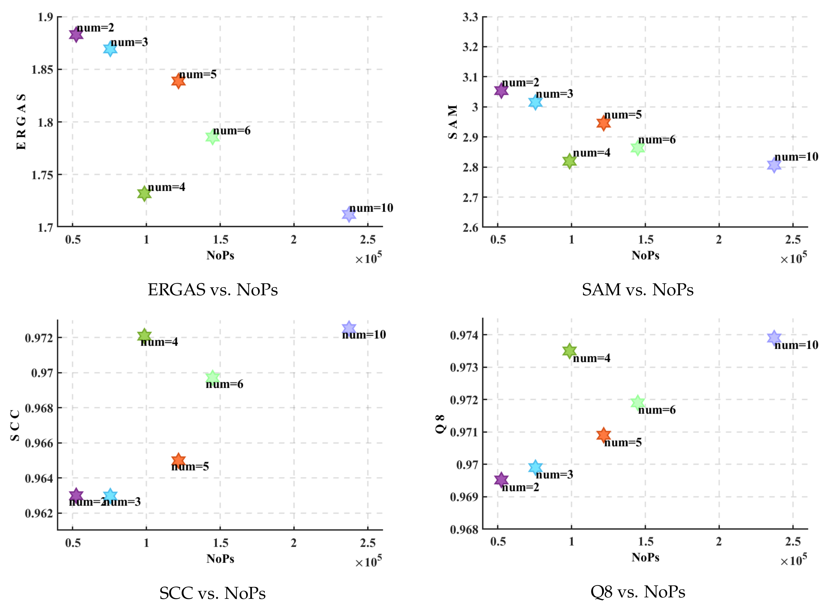
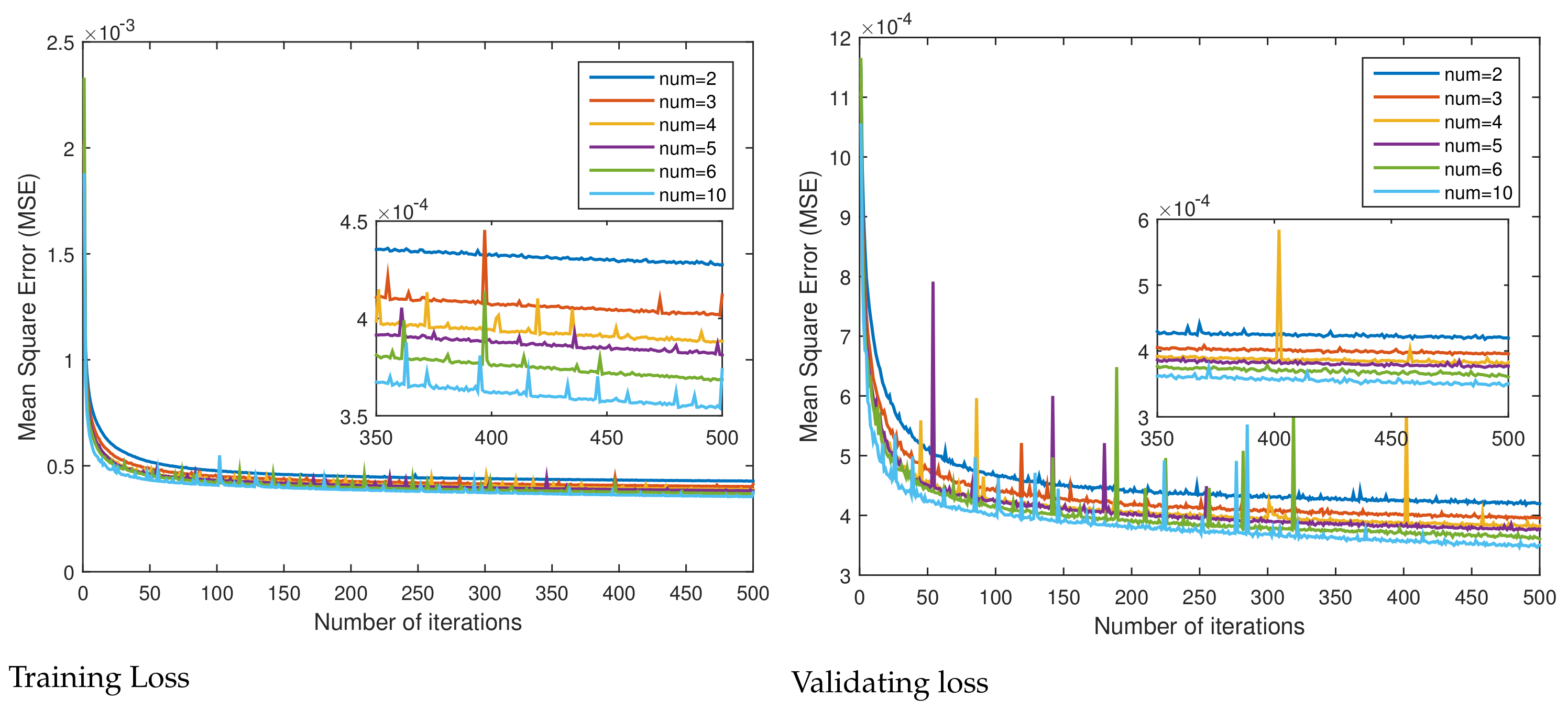
Given that the dominant point of this paper is the introduction of the PFFB, what we need to discuss first is to compare the effect of the depth of the network by testing the baseline framework containing different numbers of PFFB. In this case, we set the number of PFFB from 2 to 6 and 10, respectively. As the number of modules increases and the network deepens, the amount of training parameters also increases correspondingly. Figure 15 and Figure 16 present quantitative and parameter comparisons among the different numbers of the PFFB structure on the Rio dataset. The results show that a better performance can be obtained when the number of PFFB is larger. It is worth noting that, obviously, when the number of modules is within the range of 2 to 6, more PFFBs can better achieve the full-depth feature fusion of the network, but the memory burden is increased due to the corresponding increase in the number of parameters, leading to a slight decrease in the test results. However, when the number of PFFB is 10, the fusion performance of PFFB has greater advantages, so the training effect rises again. Therefore, in order to balance performance and efficiency, we chose a PFFB number of 4 as the default setting.

4.8.3. Number of Channels

We also test the effect of the number of channels on the MS and PAN branch. Based on the previous discussion on the number of PFFB, we set the number of blocks to 4 and the number of channels as 8, 16, 32, and 64, respectively, and carried out experiments on the Rio dataset. We also plotted the performance in each indicator with their parameters in Figure 17. Obviously, with the increase in the number of channels, the number of parameters gradually increased. Thus more spectral information could be explored. It worked best when the number of channels was 64. However, considering the pressure of a large number of parameters on the memory load, in order to balance the network performance and memory load and maximize the advantages of both, we chose 16 as the default setting of the number of channels.

4.9. Parameter Numbers

The number of parameters (NoPs) of all the compared DL-based methods are presented in

Table 9. The number of parameters (NoPs) of DL-based methods.

Method	PNN	PanNet	DiCNN1	DMDNet	FDFNet
NoPs	$1.04\times {10}^5$	$8.30\times {10}^4$	$4.68\times {10}^4$	$1.0\times {10}^5$	$9.9\times {10}^4$

. It can be seen that the amount of parameters of FDFNet has not increased much than the other compared DL-based methods, but the best results are achieved. This is because our network can perform more efficient fusion at full-depth, which leads to promising results that achieve a reasonable balance between spectral and spatial information, and also proves the efficiency of extracting features from parallel branches.

5. Conclusions

In this work, we introduced an effective full-depth feature fusion network (FDFNet) for remote sensing that contains three distinctive branches called the PAN-branch, MS-branch, and fusion-branch, respectively. The fusion of these three branches is operated at every different depth to make the information fusion more comprehensive. Furthermore, the parallel feature fusion block (PFFB) that composes FDFNet can also be treated as a basic module, which can be applied to other CNN-based structures used to solve remote sensing image fusion problems. Extensive experiments validate the superiority of our FDFNet on reduced- and full-resolution images in comparison to state-of-the-art pansharpening methods with relatively few parameters.

References

1. Alparone, L.; Wald, L.; Chanussot, J.; Thomas, C.; Gamba, P.; Bruce, L.M. Comparison of pansharpening algorithms: Outcome of the 2006 GRSS data fusion contest. IEEE Trans. Geosci. Remote Sens. 2007, 45, 3012–3021. [Google Scholar] [CrossRef] [Green Version]
2. Garzelli, A.; Nencini, F.; Capobianco, L. Optimal MMSE Pan Sharpening of Very High Resolution Multispectral Images. IEEE Trans. Geosci. Remote Sens. 2008, 46, 228–236. [Google Scholar] [CrossRef]
3. Vivone, G. Robust Band-Dependent Spatial-Detail Approaches for Panchromatic Sharpening. IEEE Trans. Geosci. Remote Sens. 2019, 57, 6421–6433. [Google Scholar] [CrossRef]
4. Choi, J.; Yu, K.; Kim, Y. A New Adaptive Component-Substitution-Based Satellite Image Fusion by Using Partial Replacement. IEEE Trans. Geosci. Remote Sens. 2011, 49, 295–309. [Google Scholar] [CrossRef]
5. Laben, C.A.; Brower, B.V. Process for Enhancing the Spatial Resolution of Multispectral Imagery Using Pan-Sharpening. U.S. Patent 6,011,875, 4 January 2000. [Google Scholar]
6. Liu, J. Smoothing filter-based intensity modulation: A spectral preserve image fusion technique for improving spatial details. Int. J. Remote Sens. 2000, 21, 3461–3472. [Google Scholar] [CrossRef]
7. Otazu, X.; González-Audícana, M.; Fors, O.; Núñez, J. Introduction of sensor spectral response into image fusion methods. Application to wavelet-based methods. IEEE Trans. Geosci. Remote Sens. 2005, 43, 2376–2385. [Google Scholar] [CrossRef] [Green Version]
8. Shensa, M.J. The discrete wavelet transform: Wedding the a trous and Mallat algorithms. IEEE Trans. Signal Process. 1992, 40, 2464–2482. [Google Scholar] [CrossRef] [Green Version]
9. Burt, P.J.; Adelson, E.H. The Laplacian pyramid as a compact image code. In Readings in Computer Vision; Elsevier: Amsterdam, The Netherlands, 1987; pp. 671–679. [Google Scholar]
10. Vivone, G.; Restaino, R.; Dalla Mura, M.; Licciardi, G.; Chanussot, J. Contrast and error-based fusion schemes for multispectral image pansharpening. IEEE Geosci. Remote Sens. Lett. 2013, 11, 930–934. [Google Scholar] [CrossRef] [Green Version]
11. Vivone, G.; Restaino, R.; Chanussot, J. Full scale regression-based injection coefficients for panchromatic sharpening. IEEE Trans. Image Process. 2018, 27, 3418–3431. [Google Scholar] [CrossRef] [PubMed]
12. Fu, X.; Lin, Z.; Huang, Y.; Ding, X. A variational pan-sharpening with local gradient constraints. In Proceedings of the IEEE/CVF Conference on Computer Vision and Pattern Recognition, Long Beach, CA, USA, 16–20 June 2019; pp. 10265–10274. [Google Scholar]
13. Chen, C.; Li, Y.; Liu, W.; Huang, J. Image fusion with local spectral consistency and dynamic gradient sparsity. In Proceedings of the IEEE Conference on Computer Vision and Pattern Recognition, Columbus, OH, USA, 24–27 June 2014; pp. 2760–2765. [Google Scholar]
14. He, X.; Condat, L.; Bioucas-Dias, J.M.; Chanussot, J.; Xia, J. A new pansharpening method based on spatial and spectral sparsity priors. IEEE Trans. Image Process. 2014, 23, 4160–4174. [Google Scholar] [CrossRef]
15. Jiang, Y.; Ding, X.; Zeng, D.; Huang, Y.; Paisley, J. Pan-sharpening with a hyper-laplacian penalty. In Proceedings of the IEEE International Conference on Computer Vision, Santiago, Chile, 7–13 December 2015; pp. 540–548. [Google Scholar]
16. Wang, T.; Fang, F.; Li, F.; Zhang, G. High-quality Bayesian pansharpening. IEEE Trans. Image Process. 2018, 28, 227–239. [Google Scholar] [CrossRef]
17. Moeller, M.; Wittman, T.; Bertozzi, A.L. A variational approach to hyperspectral image fusion. Proc. SPIE 2009, 7334, 73341E. [Google Scholar] [CrossRef] [Green Version]
18. Fang, F.; Li, F.; Shen, C.; Zhang, G. A Variational Approach for Pan-Sharpening. IEEE Trans. Image Process. 2013, 22, 2822–2834. [Google Scholar] [CrossRef] [PubMed]
19. Duran, J.; Buades, A.; Coll, B.; Sbert, C. A nonlocal variational model for pansharpening image fusion. SIAM J. Imaging Sci. 2014, 7, 761–796. [Google Scholar] [CrossRef]
20. Palsson, F.; Sveinsson, J.R.; Ulfarsson, M.O. A new pansharpening algorithm based on total variation. IEEE Geosci. Remote Sens. Lett. 2013, 11, 318–322. [Google Scholar] [CrossRef]
21. Aly, H.A.; Sharma, G. A regularized model-based optimization framework for pan-sharpening. IEEE Trans. Image Process. 2014, 23, 2596–2608. [Google Scholar] [CrossRef] [Green Version]
22. Chen, C.; Li, Y.; Liu, W.; Huang, J. SIRF: Simultaneous satellite image registration and fusion in a unified framework. IEEE Trans. Image Process. 2015, 24, 4213–4224. [Google Scholar] [CrossRef] [Green Version]
23. Vivone, G.; Simões, M.; Dalla Mura, M.; Restaino, R.; Bioucas-Dias, J.M.; Licciardi, G.A.; Chanussot, J. Pansharpening based on semiblind deconvolution. IEEE Trans. Geosci. Remote Sens. 2014, 53, 1997–2010. [Google Scholar] [CrossRef]
24. Wei, Q.; Dobigeon, N.; Tourneret, J.Y.; Bioucas-Dias, J.; Godsill, S. R-FUSE: Robust fast fusion of multiband images based on solving a Sylvester equation. IEEE Signal Process. Lett. 2016, 23, 1632–1636. [Google Scholar] [CrossRef] [Green Version]
25. Deng, L.J.; Vivone, G.; Guo, W.; Dalla Mura, M.; Chanussot, J. A variational pansharpening approach based on reproducible kernel Hilbert space and heaviside function. IEEE Trans. Image Process. 2018, 27, 4330–4344. [Google Scholar] [CrossRef]
26. Zhang, Z.Y.; Huang, T.Z.; Deng, L.J.; Huang, J.; Zhao, X.L.; Zheng, C.C. A framelet-based iterative pan-sharpening approach. Remote Sens. 2018, 10, 622. [Google Scholar] [CrossRef] [Green Version]
27. Vivone, G.; Addesso, P.; Restaino, R.; Dalla Mura, M.; Chanussot, J. Pansharpening based on deconvolution for multiband filter estimation. IEEE Trans. Geosci. Remote Sens. 2018, 57, 540–553. [Google Scholar] [CrossRef]
28. Xu, T.; Huang, T.Z.; Deng, L.J.; Zhao, X.L.; Huang, J. Hyperspectral image superresolution using unidirectional total variation with tucker decomposition. IEEE J. Sel. Top. Appl. Earth Obs. Remote Sens. 2020, 13, 4381–4398. [Google Scholar] [CrossRef]
29. Deng, L.J.; Feng, M.; Tai, X.C. The fusion of panchromatic and multispectral remote sensing images via tensor-based sparse modeling and hyper-Laplacian prior. Inf. Fusion 2019, 52, 76–89. [Google Scholar] [CrossRef]
30. Li, S.; Yang, B. A new pan-sharpening method using a compressed sensing technique. IEEE Trans. Geosci. Remote Sens. 2010, 49, 738–746. [Google Scholar] [CrossRef]
31. Zhu, X.X.; Bamler, R. A sparse image fusion algorithm with application to pan-sharpening. IEEE Trans. Geosci. Remote Sens. 2012, 51, 2827–2836. [Google Scholar] [CrossRef]
32. Vicinanza, M.R.; Restaino, R.; Vivone, G.; Dalla Mura, M.; Chanussot, J. A pansharpening method based on the sparse representation of injected details. IEEE Geosci. Remote Sens. Lett. 2014, 12, 180–184. [Google Scholar] [CrossRef]
33. Liu, J.; Zhou, C.; Fei, R.; Zhang, C.; Zhang, J. Pansharpening Via Neighbor Embedding of Spatial Details. IEEE J. Sel. Top. Appl. Earth Obs. Remote Sens. 2021, 14, 4028–4042. [Google Scholar] [CrossRef]
34. Fu, X.; Wang, W.; Huang, Y.; Ding, X.; Paisley, J. Deep multiscale detail networks for multiband spectral image sharpening. IEEE Trans. Neural Netw. Learn. Syst. 2020, 32, 2090–2104. [Google Scholar] [CrossRef]
35. Yang, J.; Fu, X.; Hu, Y.; Huang, Y.; Ding, X.; Paisley, J. PanNet: A deep network architecture for pan-sharpening. In Proceedings of the IEEE International Conference on Computer Vision, Venice, Italy, 22–29 October 2017; pp. 5449–5457. [Google Scholar]
36. He, L.; Rao, Y.; Li, J.; Chanussot, J.; Plaza, A.; Zhu, J.; Li, B. Pansharpening via detail injection based convolutional neural networks. IEEE J. Sel. Top. Appl. Earth Obs. Remote Sens. 2019, 12, 1188–1204. [Google Scholar] [CrossRef] [Green Version]
37. Masi, G.; Cozzolino, D.; Verdoliva, L.; Scarpa, G. Pansharpening by convolutional neural networks. Remote Sens. 2016, 8, 594. [Google Scholar] [CrossRef] [Green Version]
38. Deng, L.J.; Vivone, G.; Jin, C.; Chanussot, J. Detail Injection-Based Deep Convolutional Neural Networks for Pansharpening. IEEE Trans. Geosci. Remote Sens. 2021, 59, 6995–7010. [Google Scholar] [CrossRef]
39. Liu, J.; Feng, Y.; Zhou, C.; Zhang, C. Pwnet: An adaptive weight network for the fusion of panchromatic and multispectral images. Remote Sens. 2020, 12, 2804. [Google Scholar] [CrossRef]
40. Wang, Y.; Xu, S.; Liu, J.; Zhao, Z.; Zhang, C.; Zhang, J. MFIF-GAN: A new generative adversarial network for multi-focus image fusion. Signal Process. Image Commun. 2021, 96, 116295. [Google Scholar] [CrossRef]
41. Zhang, Y.; Liu, C.; Sun, M.; Ou, Y. Pan-sharpening using an efficient bidirectional pyramid network. IEEE Trans. Geosci. Remote Sens. 2019, 57, 5549–5563. [Google Scholar] [CrossRef]
42. Jin, C.; Deng, L.J.; Huang, T.Z.; Vivone, G. Laplacian pyramid networks: A new approach for multispectral pansharpening. Inf. Fusion 2022, 78, 158–170. [Google Scholar] [CrossRef]
43. Restaino, R.; Vivone, G.; Addesso, P.; Chanussot, J. A pansharpening approach based on multiple linear regression estimation of injection coefficients. IEEE Geosci. Remote Sens. Lett. 2019, 17, 102–106. [Google Scholar] [CrossRef]
44. Vivone, G.; Marano, S.; Chanussot, J. Pansharpening: Context-based generalized laplacian pyramids by robust regression. IEEE Trans. Geosci. Remote Sens. 2020, 58, 6152–6167. [Google Scholar] [CrossRef]
45. Wang, Y.T.; Zhao, X.L.; Jiang, T.X.; Deng, L.J.; Chang, Y.; Huang, T.Z. Rain Streaks Removal for Single Image via Kernel-Guided Convolutional Neural Network. IEEE Trans. Neural Netw. Learn. Syst. 2021, 32, 3664–3676. [Google Scholar] [CrossRef] [PubMed]
46. Ledig, C.; Theis, L.; Huszár, F.; Caballero, J.; Cunningham, A.; Acosta, A.; Aitken, A.; Tejani, A.; Totz, J.; Wang, Z.; et al. Photo-realistic single image super-resolution using a generative adversarial network. In Proceedings of the IEEE Conference on Computer Vision and Pattern Recognition, Honolulu, HI, USA, 21–26 July 2017; pp. 4681–4690. [Google Scholar]
47. Dong, C.; Loy, C.C.; He, K.; Tang, X. Image super-resolution using deep convolutional networks. IEEE Trans. Pattern Anal. Mach. Intell. 2015, 38, 295–307. [Google Scholar] [CrossRef] [Green Version]
48. Dong, C.; Loy, C.C.; He, K.; Tang, X. Learning a deep convolutional network for image super-resolution. In European Conference on Computer Vision; Springer: Berlin/Heidelberg, Germany, 2014; pp. 184–199. [Google Scholar]
49. Lim, B.; Son, S.; Kim, H.; Nah, S.; Mu Lee, K. Enhanced deep residual networks for single image super-resolution. In Proceedings of the IEEE Conference on Computer Vision and Pattern Recognition Workshops, Honolulu, HI, USA, 21–26 July 2017; pp. 136–144. [Google Scholar]
50. Redmon, J.; Farhadi, A. Yolov3: An incremental improvement. arXiv 2018, arXiv:1804.02767. [Google Scholar]
51. Bochkovskiy, A.; Wang, C.Y.; Liao, H.Y.M. Yolov4: Optimal speed and accuracy of object detection. arXiv 2020, arXiv:2004.10934. [Google Scholar]
52. He, K.; Gkioxari, G.; Dollár, P.; Girshick, R. Mask r-cnn. In Proceedings of the IEEE International Conference on Computer Vision, Venice, Italy, 22–29 October 2017; pp. 2961–2969. [Google Scholar]
53. Hu, J.F.; Huang, T.Z.; Deng, L.J.; Jiang, T.X.; Vivone, G.; Chanussot, J. Hyperspectral Image Super-Resolution via Deep Spatiospectral Attention Convolutional Neural Networks. IEEE Trans. Neural Netw. Learn. Syst. 2021, 1–15. [Google Scholar] [CrossRef] [PubMed]
54. Wu, Z.C.; Huang, T.Z.; Deng, L.J.; Hu, J.F.; Vivone, G. VO+Net: An Adaptive Approach Using Variational Optimization and Deep Learning for Panchromatic Sharpening. IEEE Trans. Geosci. Remote Sens. 2021, 60, 1–16. [Google Scholar] [CrossRef]
55. Wu, Z.C.; Huang, T.Z.; Deng, L.J.; Vivone, G.; Miao, J.Q.; Hu, J.F.; Zhao, X.L. A new variational approach based on proximal deep injection and gradient intensity similarity for spatio-spectral image fusion. IEEE J. Sel. Top. Appl. Earth Obs. Remote Sens. 2020, 13, 6277–6290. [Google Scholar] [CrossRef]
56. Dian, R.; Li, S. Hyperspectral image super-resolution via subspace-based low tensor multi-rank regularization. IEEE Trans. Image Process. 2019, 28, 5135–5146. [Google Scholar] [CrossRef] [PubMed]
57. Dian, R.; Li, S.; Kang, X. Regularizing hyperspectral and multispectral image fusion by CNN denoiser. IEEE Trans. Neural Netw. Learn. Syst. 2020, 32, 1124–1135. [Google Scholar] [CrossRef]
58. Cao, X.; Yao, J.; Xu, Z.; Meng, D. Hyperspectral Image Classification With Convolutional Neural Network and Active Learning. IEEE Trans. Geosci. Remote Sens. 2020, 58, 4604–4616. [Google Scholar] [CrossRef]
59. Cao, X.; Fu, X.; Xu, C.; Meng, D. Deep Spatial-Spectral Global Reasoning Network for Hyperspectral Image Denoising. IEEE Trans. Geosci. Remote Sens. 2021, 60. [Google Scholar] [CrossRef]
60. Yuan, Q.; Wei, Y.; Meng, X.; Shen, H.; Zhang, L. A multiscale and multidepth convolutional neural network for remote sensing imagery pan-sharpening. IEEE J. Sel. Top. Appl. Earth Obs. Remote Sens. 2018, 11, 978–989. [Google Scholar] [CrossRef] [Green Version]
61. Wei, Y.; Yuan, Q.; Shen, H.; Zhang, L. Boosting the accuracy of multispectral image pansharpening by learning a deep residual network. IEEE Geosci. Remote Sens. Lett. 2017, 14, 1795–1799. [Google Scholar] [CrossRef] [Green Version]
62. Xiang, Z.; Xiao, L.; Liao, W.; Philips, W. MC-JAFN: Multilevel Contexts-Based Joint Attentive Fusion Network for Pansharpening. IEEE Geosci. Remote Sens. Lett. 2021, 19, 1–5. [Google Scholar] [CrossRef]
63. Liu, P.; Xiao, L. A Nonconvex Pansharpening Model With Spatial and Spectral Gradient Difference-Induced Nonconvex Sparsity Priors. IEEE Trans. Geosci. Remote Sens. 2021, 60, 1–15. [Google Scholar] [CrossRef]
64. Ma, J.; Yu, W.; Chen, C.; Liang, P.; Guo, X.; Jiang, J. Pan-GAN: An unsupervised pan-sharpening method for remote sensing image fusion. Inf. Fusion 2020, 62, 110–120. [Google Scholar] [CrossRef]
65. Li, K.; Zhang, W.; Tian, X.; Ma, J.; Zhou, H.; Wang, Z. Variation-Net: Interpretable Variation-Inspired Deep Network for Pansharpening. In Proceedings of the 2021 IEEE International Conference on Multimedia and Expo (ICME), Shenzhen, China, 5–9 July 2021; pp. 1–6. [Google Scholar] [CrossRef]
66. Zhuang, P.; Liu, Q.; Ding, X. Pan-GGF: A probabilistic method for pan-sharpening with gradient domain guided image filtering. Signal Process. 2019, 156, 177–190. [Google Scholar] [CrossRef]
67. Guo, P.; Zhuang, P.; Guo, Y. Bayesian pan-sharpening with multiorder gradient-based deep network constraints. IEEE J. Sel. Top. Appl. Earth Obs. Remote Sens. 2020, 13, 950–962. [Google Scholar] [CrossRef]
68. Yang, Y.; Wu, L.; Huang, S.; Wan, W.; Tu, W.; Lu, H. Multiband remote sensing image pansharpening based on dual-injection model. IEEE J. Sel. Top. Appl. Earth Obs. Remote Sens. 2020, 13, 1888–1904. [Google Scholar] [CrossRef]
69. Yang, Y.; Lu, H.; Huang, S.; Tu, W. Pansharpening Based on Joint-Guided Detail Extraction. IEEE J. Sel. Top. Appl. Earth Obs. Remote Sens. 2020, 14, 389–401. [Google Scholar] [CrossRef]
70. Lei, D.; Huang, Y.; Zhang, L.; Li, W. Multibranch Feature Extraction and Feature Multiplexing Network for Pansharpening. IEEE Trans. Geosci. Remote Sens. 2021, 59, 2231–2244. [Google Scholar] [CrossRef]
71. Hu, J.; Hu, P.; Kang, X.; Zhang, H.; Fan, S. Pan-sharpening via multiscale dynamic convolutional neural network. IEEE Trans. Geosci. Remote Sens. 2020, 59, 2231–2244. [Google Scholar] [CrossRef]
72. Scarpa, G.; Vitale, S.; Cozzolino, D. Target-adaptive CNN-based pansharpening. IEEE Trans. Geosci. Remote Sens. 2018, 56, 5443–5457. [Google Scholar] [CrossRef] [Green Version]
73. Zhang, H.; Ma, J. GTP-PNet: A residual learning network based on gradient transformation prior for pansharpening. ISPRS J. Photogramm. Remote Sens. 2021, 172, 223–239. [Google Scholar] [CrossRef]
74. Hu, J.; Du, C.; Fan, S. Two-stage pansharpening based on multi-level detail injection network. IEEE Access 2020, 8, 156442–156455. [Google Scholar] [CrossRef]
75. Ozcelik, F.; Alganci, U.; Sertel, E.; Unal, G. Rethinking CNN-based pansharpening: Guided colorization of panchromatic images via GANS. IEEE Trans. Geosci. Remote Sens. 2020, 59, 3486–3501. [Google Scholar] [CrossRef]
76. Aiazzi, B.; Alparone, L.; Baronti, S.; Garzelli, A. Context-driven fusion of high spatial and spectral resolution images based on oversampled multiresolution analysis. IEEE Trans. Geosci. Remote Sens. 2002, 40, 2300–2312. [Google Scholar] [CrossRef]
77. Wald, L.; Ranchin, T.; Mangolini, M. Fusion of satellite images of different spatial resolutions: Assessing the quality of resulting images. Photogramm. Eng. Remote Sens. 1997, 63, 691–699. [Google Scholar]
78. Kingma, D.P.; Ba, J. Adam: A method for stochastic optimization. arXiv 2014, arXiv:1412.6980. [Google Scholar]
79. Yokoya, N.; Yairi, T.; Iwasaki, A. Coupled nonnegative matrix factorization unmixing for hyperspectral and multispectral data fusion. IEEE Trans. Geosci. Remote Sens. 2011, 50, 528–537. [Google Scholar] [CrossRef]
80. Wald, L. Data Fusion: Definitions and Architectures: Fusion of Images of Different Spatial Resolutions; Les Presses de l’Ecole des Mines de Paris: Paris, France, 2002. [Google Scholar]
81. Yuhas, R.H.; Goetz, A.F.; Boardman, J.W. Discrimination among Semi-Arid Landscape Endmembers Using the Spectral Angle Mapper (SAM) Algorithm. 1992. Available online: https://aviris.jpl.nasa.gov/proceedings/workshops/92_docs/52.PDF (accessed on 6 April 2021).
82. Zhou, J.; Civco, D.; Silander, J. A wavelet transform method to merge Landsat TM and SPOT panchromatic data. Int. J. Remote Sens. 1998, 19, 743–757. [Google Scholar] [CrossRef]
83. Garzelli, A.; Nencini, F. Hypercomplex quality assessment of multi/hyperspectral images. IEEE Geosci. Remote Sens. Lett. 2009, 6, 662–665. [Google Scholar] [CrossRef]
84. Vivone, G.; Alparone, L.; Chanussot, J.; Dalla Mura, M.; Garzelli, A.; Licciardi, G.A.; Restaino, R.; Wald, L. A critical comparison among pansharpening algorithms. IEEE Trans. Geosci. Remote Sens. 2014, 53, 2565–2586. [Google Scholar] [CrossRef]
85. Vivone, G.; Dalla Mura, M.; Garzelli, A.; Restaino, R.; Scarpa, G.; Ulfarsson, M.O.; Alparone, L.; Chanussot, J. A new benchmark based on recent advances in multispectral pansharpening: Revisiting pansharpening with classical and emerging pansharpening methods. IEEE Geosci. Remote Sens. Mag. 2020, 9, 53–81. [Google Scholar] [CrossRef]
Figure 1. First row: Schematic diagram of pansharpening. Pansharpening aims to fuse a low spatial resolution multispectral (MS) image and the panchromatic (PAN) image, and the ground-truth image are presented. Second row: Results presentation. The fusion images and the corresponding absolute error maps of DMDNet [34] and the proposed FDFNet.
Remotesensing 14 00466 g001
Figure 2. The overall architecture of the proposed full-depth feature Fusion Network (FDFNet). Please note that the kernel size of the convolution in FDFNet is 3 × 3, the channels of the PAN branch and MS branch is 16, and the channels of fusion branch is 32. For more details, please refer to Section 3.2.
Remotesensing 14 00466 g002
Figure 3. Detailed illustration of the parallel feature fusion block (PFFB).
Remotesensing 14 00466 g003
Figure 4. Schematic diagram of the average value of all bands in the feature map after normalization. The placement order is from left to right in accordance with the output order.
Remotesensing 14 00466 g004
Figure 5. The visual comparisons of fusion results obtained by different methods on a reduced-resolution Rio dataset obtained by WorldView-3 (shown by bands: 1, 3, and 5).
Remotesensing 14 00466 g005
Figure 6. The visual comparisons of the corresponding residual maps using the GT image as reference (shown by bands: 1, 3, and 5).
Remotesensing 14 00466 g006
Figure 7. The visual comparisons of fusion results obtained by different methods on a reduced-resolution QB case (shown by bands: 1, 3, and 5).
Remotesensing 14 00466 g007
Figure 8. The visual comparisons of fusion results obtained by different methods on a reduced-resolution GF case (shown by bands: 1, 3, and 5).
Remotesensing 14 00466 g008
Figure 9. The visual comparisons of the corresponding residual maps using the GT image as reference (shown by bands: 1, 3, and 5).
Remotesensing 14 00466 g009
Figure 10. The visual comparisons of the corresponding residual maps using the GT image as reference (shown by bands: 1, 3, and 5).
Remotesensing 14 00466 g010
Figure 11. The visual comparisons on a full-resolution WorldView-3 case (shown by bands: 1, 3, and 5).
Remotesensing 14 00466 g011
Figure 12. The visual comparisons on a full-resolution WorldView-3 case (shown by bands: 1, 3, and 5).
Remotesensing 14 00466 g012
Figure 13. The visual comparisons on a full-resolution QB case (shown by bands: 1, 3, and 4).
Remotesensing 14 00466 g013
Figure 14. The visual comparisons on a full-resolution GaoFen-2 case (shown by bands: 1, 3, and 4).
Remotesensing 14 00466 g014
Figure 15. Number of parameters (NoPs) report and quantitative comparison of the number of PFFBs on the Rio dataset.
Remotesensing 14 00466 g015
Figure 16. Convergence of different numbers of the PFFB structure: Training loss and validating loss.
Remotesensing 14 00466 g016
Figure 17. Number of parameters (NoPs) report and quantitative comparison of the number of channels on the Rio dataset.
Remotesensing 14 00466 g017