Author Contributions
Conceptualization, A.F. and I.R.; methodology, A.F. and A.S.; software, A.F. and A.S.; formal analysis, A.F.; investigation, A.F. and A.S.; resources, I.R.; data curation, A.F.; writing—original draft preparation, A.F., A.S.; writing—review and editing, A.F., I.R. All authors have read and agreed to the published version of the manuscript.
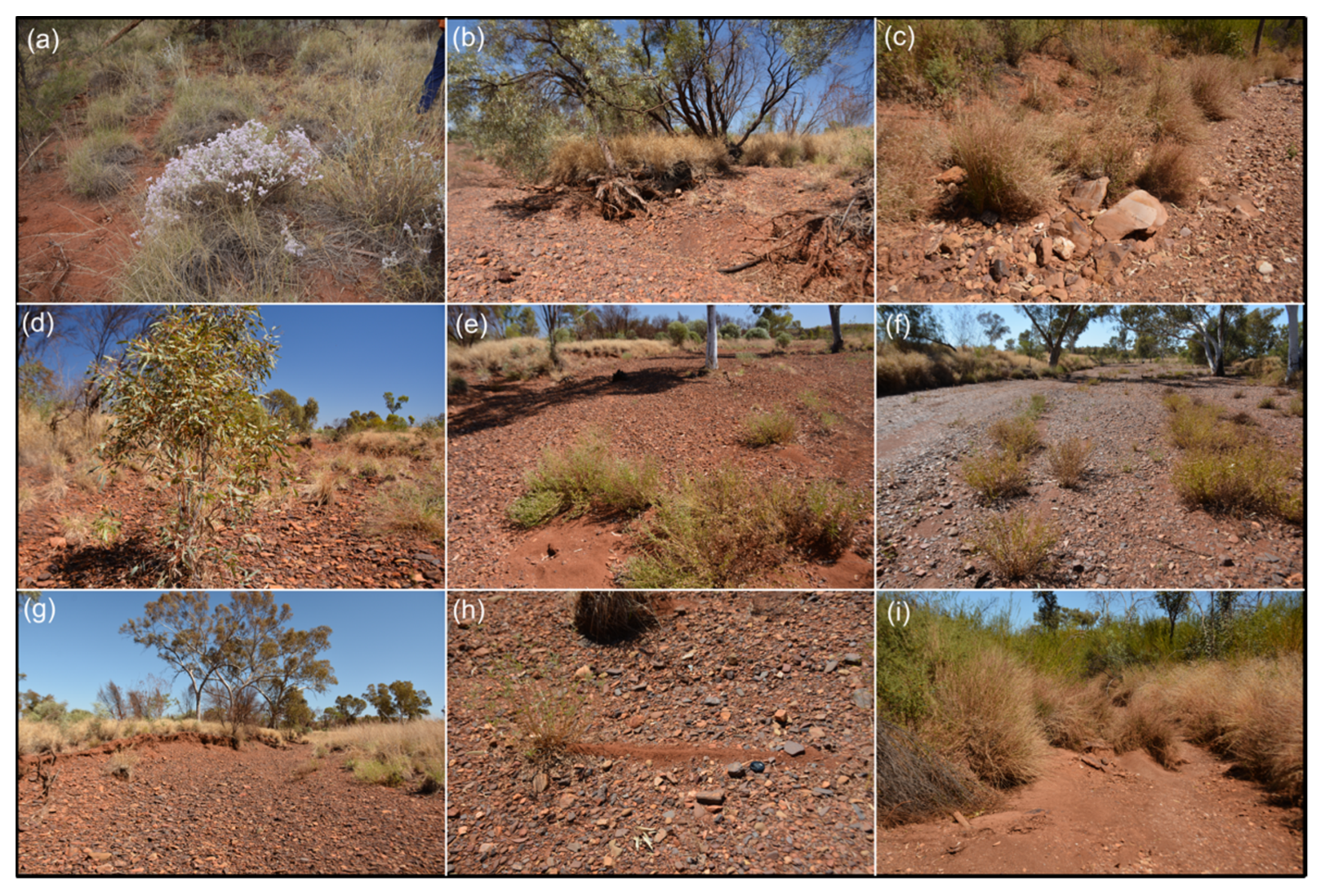
Figure 1.
Vegetation found within the headwater channels in the Pilbara region: (a) cotton bush (Ptilotus obovatus) and hard spinifex (Triodia lanigera), (b) LWD in a cobble substrate, (c) soft spinifex and buffel grass in a cobble bed, (d) young tree, (e) small shrubs and fine sediment in a cobble channel, (f) vegetation in a cobble substrate, (g) eucalyptus tree surrounded by soft spinifex, (h) narrow ridge-bar, (i) highly vegetated sand-bed channel.
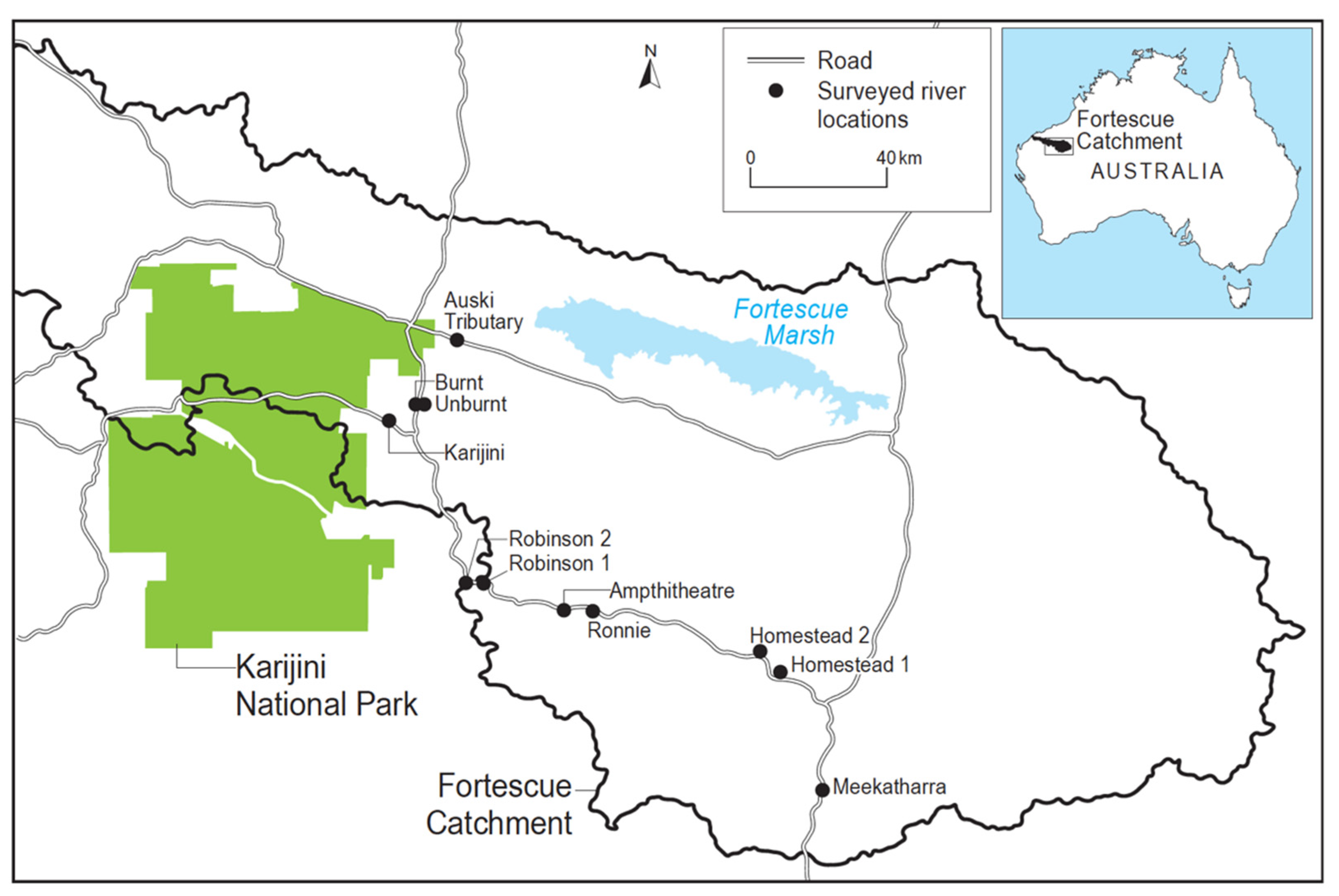
Figure 2.
Map of surveyed channels in the Upper Fortescue Catchment, in the Pilbara, Western Australia.
Figure 2.
Map of surveyed channels in the Upper Fortescue Catchment, in the Pilbara, Western Australia.
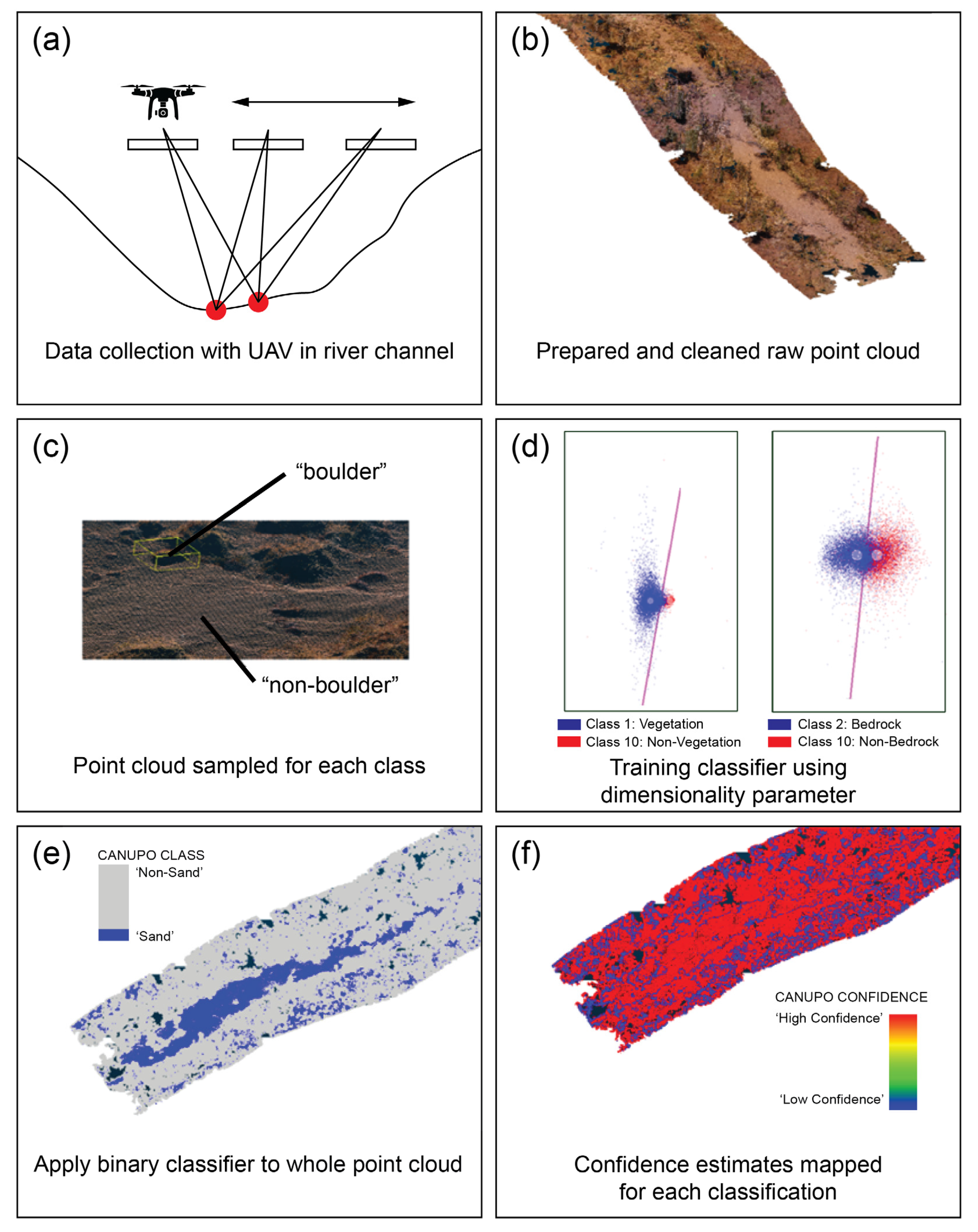
Figure 3.
CANUPO procedure diagram. (a) Data collection from UAV, (b) dense point cloud of river reach, (c) classes are discriminated in the point cloud and partitioned. (d) Classes are defined to create a classifier file, where points are discriminated using dimensionality parameters across a defined series of scales to decide “class one” or “class two,” (e) classifier file is then applied to a whole point cloud, (f) confidence estimate is mapped for the classification to show areas of high and low confidence.
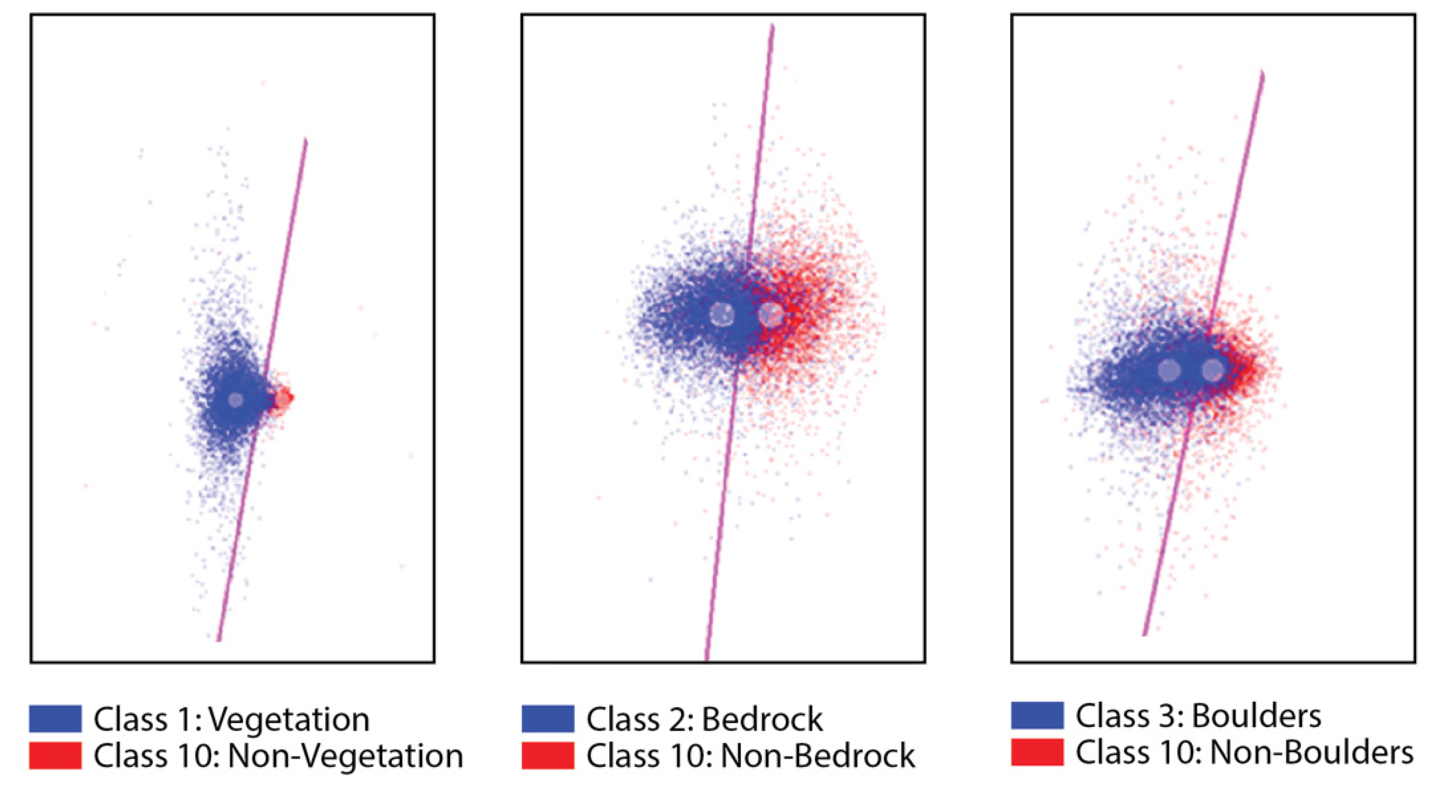
Figure 4.
Semi-supervised classifier training result for identified features within natural channels. Data are projected in the plain of maximal separability and the spheres represent each class in the plane of maximal separability. The classification boundary is represented by magenta line and the core points extracted from the point cloud are shown. Greater point mixing between this line indicates a poorer performing classifier file. Class 1 shows vegetation and non-vegetation, a strong performing classifier file with little overlap between the classification boundary.
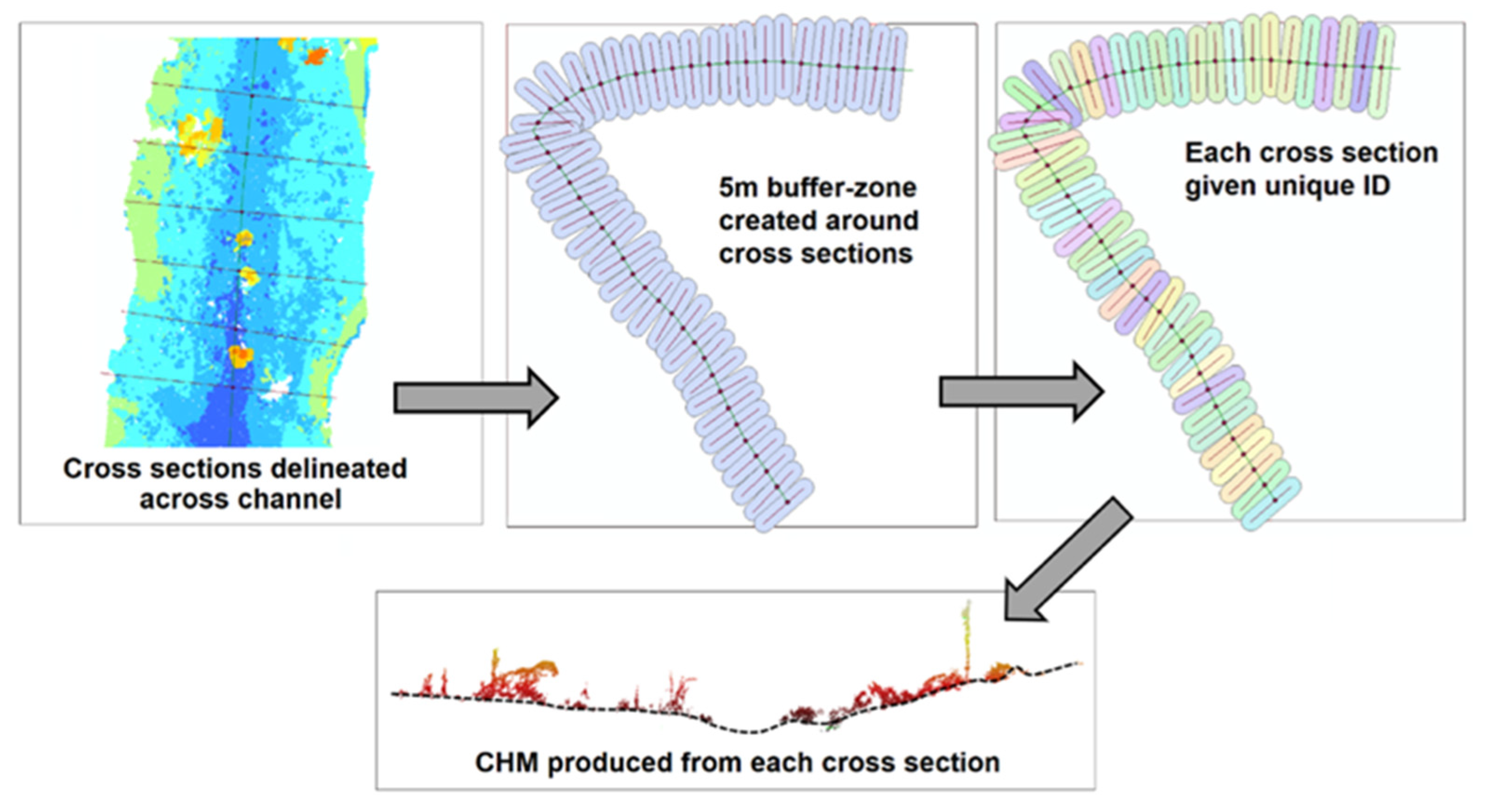
Figure 5.
Process of creating CHMs at each cross section. First the cross sections are defined, buffer zones are created around each cross section and given a unique ID, then the point clouds are clipped around each buffer to create these unique CHMs at each cross section.
Figure 5.
Process of creating CHMs at each cross section. First the cross sections are defined, buffer zones are created around each cross section and given a unique ID, then the point clouds are clipped around each buffer to create these unique CHMs at each cross section.
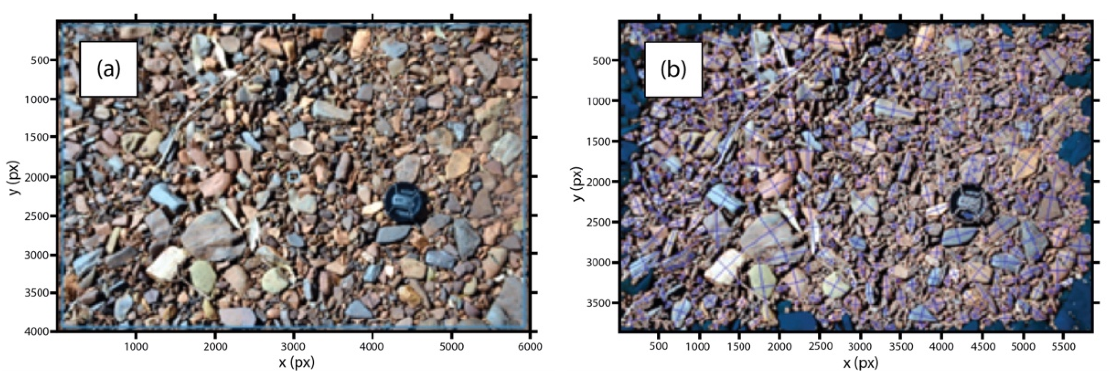
Figure 6.
BASEGRAIN software images (a) shows the raw image input and (b) shows the detection of intermediate and long axis. Sediment clasts that intersect the analysis frame are darkened here and removed from the measurement.
Figure 6.
BASEGRAIN software images (a) shows the raw image input and (b) shows the detection of intermediate and long axis. Sediment clasts that intersect the analysis frame are darkened here and removed from the measurement.
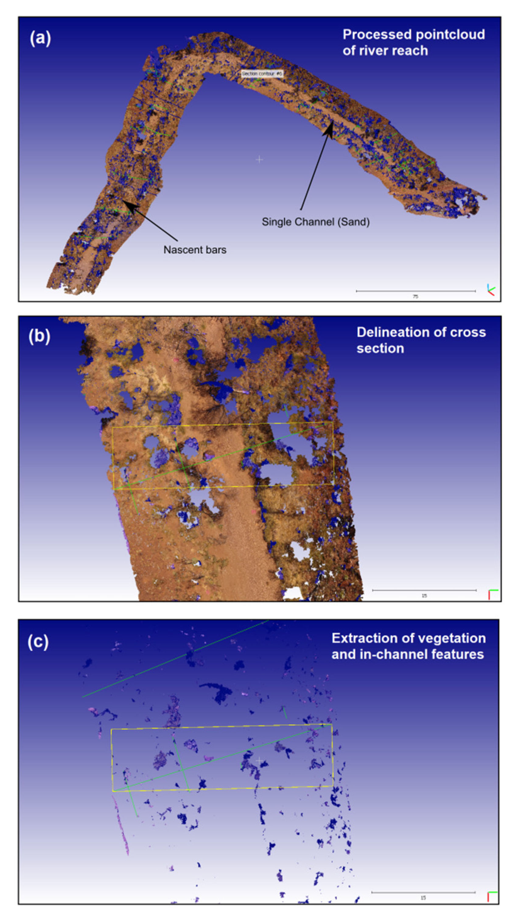
Figure 7.
Illustration showing the point cloud processing steps for the estimation of the contribution of vegetation to channel roughness (using an equation from Petryk and Bosmajian, 1975). (a) shows a processed poincloud of the river reach with geomorphic features identified, (b) highlights the delineation of cross section and (c) shows the extraction of vegetation along the cross section.
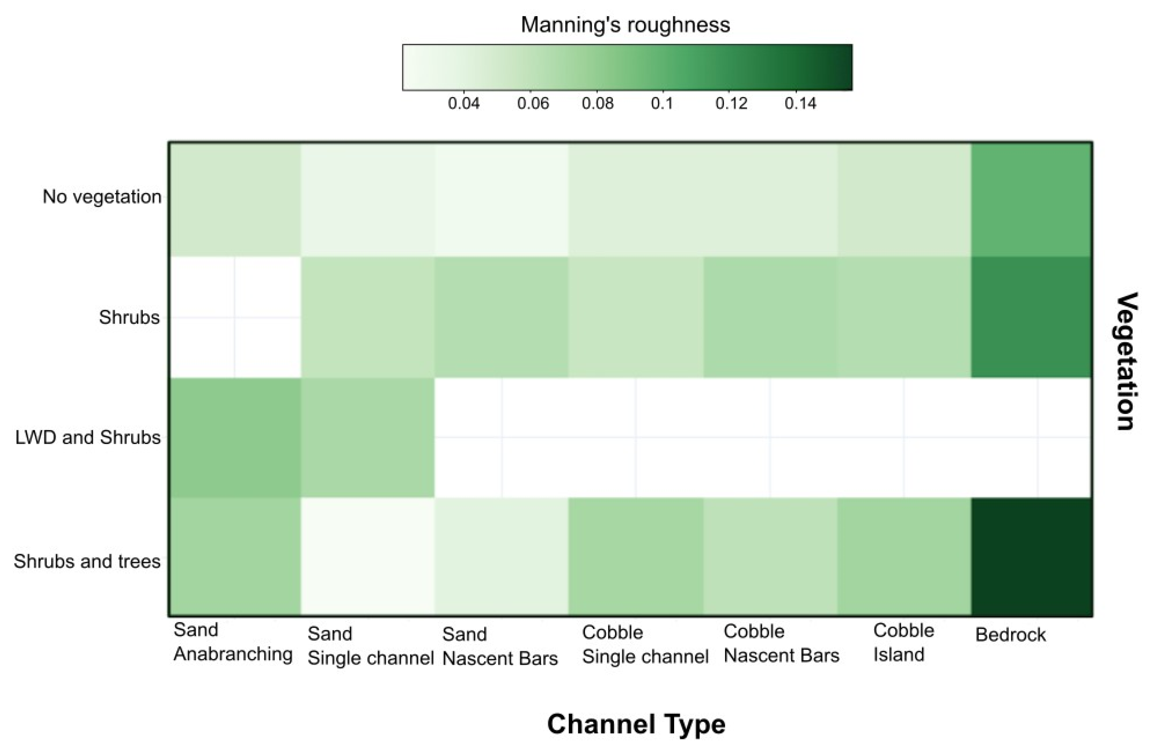
Figure 8.
Heatmap to show the relative contribution of different vegetation classes to each of the seven channel types. Darker green indicates that a greater proportion of total roughness is derived from the respective vegetation type, lighter green indicates a smaller proportion of total roughness is derived from the respective vegetation class. White indicates no value, where the channel type and associated vegetation pattern was not observed.
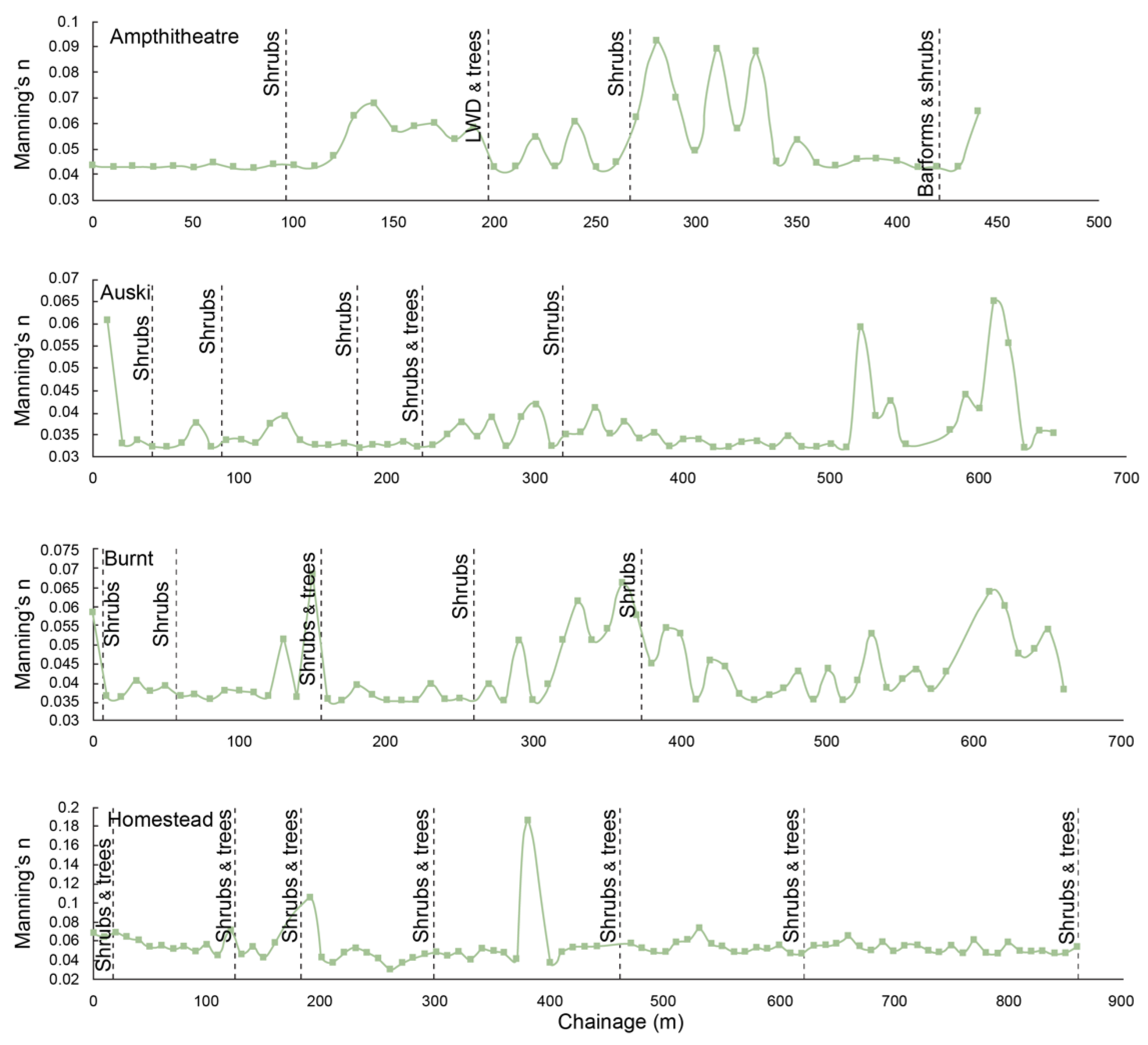
Figure 9.
Longitudinal variations in channel roughness for selected channels.
Figure 9.
Longitudinal variations in channel roughness for selected channels.
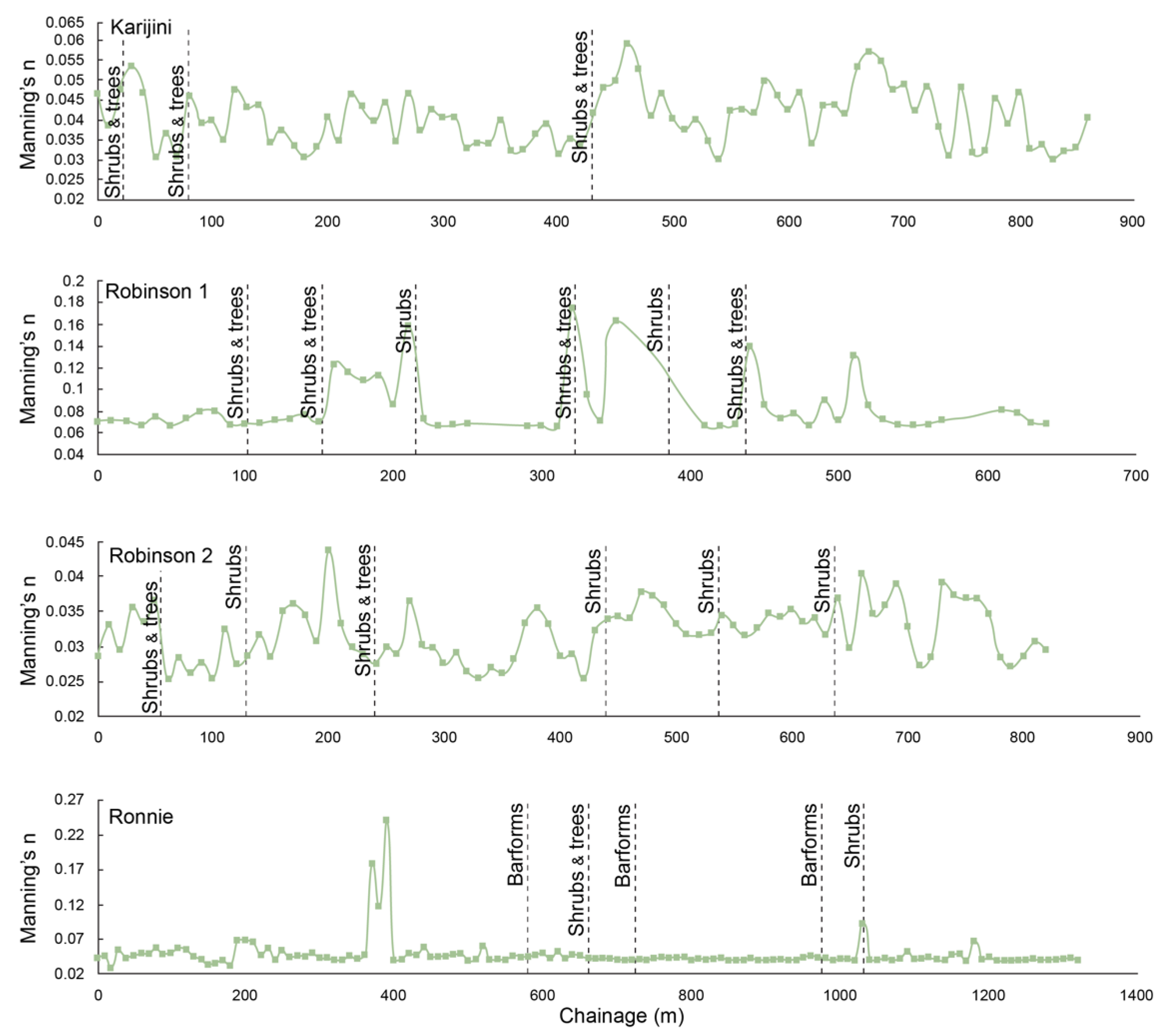
Figure 10.
Longitudinal variations in channel roughness for selected channels.
Figure 10.
Longitudinal variations in channel roughness for selected channels.
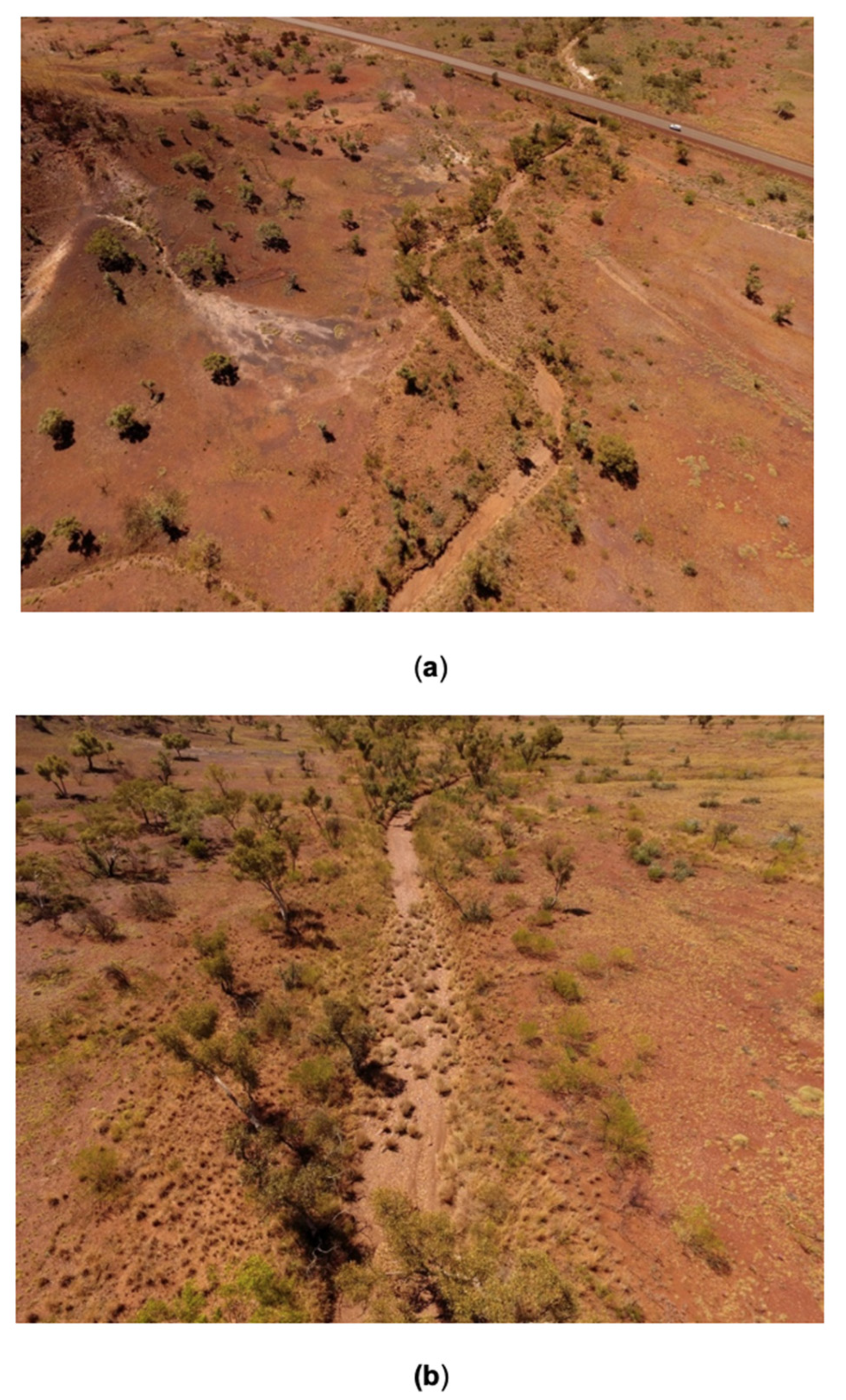
Figure 11.
Examples of headwater channel surveyed, (a) vegetated headwater channel, (b) nascent in-channel vegetation increasing channel heterogeneity within a straight river reach.
Figure 11.
Examples of headwater channel surveyed, (a) vegetated headwater channel, (b) nascent in-channel vegetation increasing channel heterogeneity within a straight river reach.
Table 1.
Geomorphic features associated with defined channel types.
Table 1.
Geomorphic features associated with defined channel types.
| Channel Type | Features Present | Features Absent |
|---|
| Single channel | Vegetation, boulders, LWD | Sand, bedrock, channel bar |
| Single channel (sand) | Vegetation, sand | Bedrock, channel bar, LWD, boulder |
| Single bedrock | Bedrock, vegetation, | Sand, channel bar, LWD, boulder |
| Bar (island) | Vegetation, boulders, sand, LWD, channel bar | Bedrock |
| Bar (Nascent) | Vegetation, channel bar, LWD, boulder, sand | Bedrock |
| Multithread | Vegetation, LWD, sand, | Bedrock, boulder, channel bar |
Table 2.
SfM survey accuracy for catchments.
Table 2.
SfM survey accuracy for catchments.
| Reach | Survey Area (km2) | Sampling Distance (cm) | Point Density (per m3) | RMSEz (m) | GCP Total |
|---|
| Amphitheatre | 0.018 | 0.89 | 3011.18 | 0.065 | 19 |
| Auski | 0.026 | 0.73 | 792.4 | * | * |
| Burnt | 0.16 | 1.5 | 664.8 | 0.035 | 40 |
| Homestead | 0.29 | 1.89 | 500.22 | 0.344 | 12 |
| Karijini | 0.0532 | 0.89 | 1861.98 | * | * |
| Meekatharra | 0.06 | 1.2 | 992.04 | * | * |
| Robinson 1 | 0.053 | 1.39 | 850 | * | 27 |
| Robinson 2 | 0.027 | 0.78 | 2187.4 | 0.058 | 29 |
| Ronnie | 0.07 | 0.93 | 1586.65 | 0.056 | 48 |
| Unburnt | 0.033 | 1.45 | 637 | * | * |
Table 3.
Results for the geomorphic classification of natural channels. Values show the results of classifier files for a subset of 10,000 point cloud points.
Table 3.
Results for the geomorphic classification of natural channels. Values show the results of classifier files for a subset of 10,000 point cloud points.
| Class Type | # | Truly Classified (%) | Falsely Classified (%) | ba | Distance to Boundary | fdr |
|---|
| Vegetated | 1 | 70 | 30 | | −7.590 ± 4.568 | |
| Non-vegetated | 10 | 95 | 5 | 0.958 | 5.964 ± 2.880 | 6.30 |
| Bedrock | 2 | 86 | 14 | | −1.441 ± 1.677 | |
| Non-bedrock | 10 | 66 | 34 | 0.760 | 2.074 ± 3.320 | 0.89 |
| Boulder | 3 | 73 | 27 | | −0.724 ± 1.176 | |
| Non-boulder | 10 | 67 | 33 | 0.702 | 0.669 ± 1.552 | 0.51 |
| Sand | 4 | 86 | 14 | | 1.758 ± 1.640 | |
| Non-sand | 10 | 79 | 21 | 0.825 | 5.004 ± 5.450 | 1.41 |
| LWD | 5 | 88 | 12 | | −2.312 ± 2.012 | |
| Non-LWD | 10 | 69 | 31 | 0.783 | 0.730 ± 1.994 | 1.15 |
| Channel bar | 6 | 72 | 28 | | −0.287 ± 0.660 | |
| Non-channel bar | 10 | 50 | 50 | 0.606 | 0.072 ± 0.733 | 0.13 |
Table 4.
River reach characteristics as calculated from SfM-derived point clouds and BASEGRAIN sediment analysis. Mean D50 and D84 values from each surveyed channel are shown.
Table 4.
River reach characteristics as calculated from SfM-derived point clouds and BASEGRAIN sediment analysis. Mean D50 and D84 values from each surveyed channel are shown.
| Channel | Reach Types | Mean Slope (m/m) | D50 (mm) | D84 (mm) | Mean W/D |
|---|
| Amphitheatre | Alluvial channel (≥cobble or sand) with nascent barforms. | 0.007 | 16.71 | 37.89 | 12.1 |
| Auski | Unconfined alluvial (≥cobble). | 0.014 | 15.38 | 28.52 | 16.94 |
| Burnt | Unconfined alluvial channel (≥cobble) and nascent barform. | 0.009 | 15.39 | 31.45 | 11.18 |
| Homestead | Unconfined alluvial channel (≥cobble) with stable island forms. | 0.005 | 18.47 | 42.088 | 15.23 |
| Karijini | Unconfined alluvial channel (≥cobble) and nascent bars. | 0.006 | 14.03 | 26.525 | 16.46 |
| Meekatharra | Unconfined single channel (sand) and stable islands (sand). | 0.003 | 2 | 4 | 24.26 |
| Robinson 1 | Bedrock channel. | 0.021 | 21.17 | 58.71 | 12.97 |
| Robinson 2 | Unconfined alluvial channel (sand) and island bars. | 0.014 | 14.16 | 22.414 | 13.04 |
| Ronnie | Unconfined alluvial (≥cobble) and barforms. | 0.0025 | 15.49 | 34.77 | 5.61 |
| Unburnt | Bedrock, alluvial single channel (≥cobble) and barforms. | 0.008 | 126.15 | 8.93 | 8.93 |
Table 5.
Manning’s values and W/D ratios for channel types using the Limerinos equation (1970).
Table 5.
Manning’s values and W/D ratios for channel types using the Limerinos equation (1970).
| Channel Type | n min | n max | Mean n 1 | Mean W/D 1 |
|---|
| Single channel (cobble) | 0.0253 | 0.2409 | 0.0427 (±0.015) | 11.731 (±7.695) |
| Single channel (sand) | 0.0044 | 0.0927 | 0.0274 (±0.023) | 18.604 (±10.788) |
| Single bedrock | 0.0661 | 0.1757 | 0.0879 (±0.032) | 12.785 (±4.353) |
| Bar (island) | 0.0252 | 0.1522 | 0.0474 (±0.022) | 19.679 (±7.679) |
| Bar (nascent) | 0.0357 | 0.0893 | 0.0461 (±0.013) | 10.272 (±4.855) |
| Multithread | 0.0324 | 0.0447 | 0.0385 (±0.004) | 27.697 (±18.269) |
Table 6.
Manning’s roughness values (n) using Phillips and Ingersoll (1998). Mean difference shows the difference between the Limerinos (1970)-derived average values of channel roughness.
Table 6.
Manning’s roughness values (n) using Phillips and Ingersoll (1998). Mean difference shows the difference between the Limerinos (1970)-derived average values of channel roughness.
| Channel Type | n min | n max | Mean n 1 | Mean Difference |
|---|
| Single channel | 0.0036 | 0.1431 | 0.0148 (±0.0097) | −0.0279 |
| Single channel (sand) | 0.0024 | 0.0450 | 0.0106 (±0.0085) | −0.0168 |
| Single bedrock | 0.0231 | 0.0058 | 0.0132 (±0.0044) | −0.0747 |
| Bar (island) | 0.0220 | 0.0047 | 0.0137 (±0.0043) | −0.0337 |
| Bar (nascent) | 0.0428 | 0.0428 | 0.0163 (±0.0083) | −0.0298 |
| Multithread | 0.0057 | 0.0157 | 0.0076 (±0.0036) | −0.0308 |
Table 7.
Contribution of in-channel vegetation to overall channel roughness in surveyed river reaches.
Table 7.
Contribution of in-channel vegetation to overall channel roughness in surveyed river reaches.
| Channel XS | Channel Type | Limerinos n | Vegetation Contribution n | Change (%) |
|---|
| Amp XS1 | Confined, alluvial, barform | 0.04264 | 0.06952 | +47.93 |
| Amp XS2 | Confined, alluvial sand | 0.042923 | 0.062041 | +36.43 |
| Amp XS3 | Semi-confined alluvial, sand | 0.042933 | 0.06993 | +47.84 |
| Amp XS4 | Semi-confined alluvial, sand | 0.0927 | 0.1348 | +37.01 |
| Amp XS5 | Semi-confined alluvial barform | 0.0429 | 0.0632 | +38.27 |
| Burnt XS1 | Unconfined alluvial barform | 0.0365 | 0.0548 | +40.09 |
| Burnt XS2 | Unconfined alluvial barform | 0.0366 | 0.0537 | +37.87 |
| Burnt XS3 | Unconfined alluvial (cobble) | 0.0355 | 0.0513 | +36.41 |
| Burnt XS4 | Unconfined alluvial (cobble) | 0.0397 | 0.0577 | +36.96 |
| Burnt XS5 | Unconfined alluvial (cobble) | 0.0451 | 0.0645 | +35.40 |
| HS XS1 | Unconfined alluvial (cobble) | 0.0687 | 0.0947 | +37.78 |
| HS XS2 | Unconfined alluvial (cobble) | 0.0697 | 0.0949 | +36.10 |
| HS XS3 | Unconfined alluvial (cobble) | 0.0611 | 0.0856 | +40.16 |
| HS XS4 | Unconfined alluvial, islands | 0.0454 | 0.0649 | +35.36 |
| HS XS5 | Unconfined alluvial, islands | 0.0571 | 0.0821 | +35.92 |
| HS XS6 | Unconfined alluvial (cobble) | 0.0550 | 0.0739 | +34.34 |
| HS XS7 | Unconfined alluvial (cobble) | 0.0477 | 0.0640 | +34.23 |
| Karijini XS1 | Unconfined alluvial (cobble) | 0.0475 | 0.0690 | +36.91 |
| Karijini XS2 | Unconfined alluvial barform | 0.0457 | 0.0659 | +36.20 |
| Karijini XS3 | Unconfined alluvial (cobble) | 0.0413 | 0.0642 | +43.41 |
| Meek XS1 | Unconfined alluvial sand barform | 0.00691 | 0.0237 | +109.70 |
| Meek XS2 | Unconfined alluvial sand barform | 0.00778 | 0.0164 | +71.30 |
| Meek XS3 | Alluvial single (sand) | 0.0109 | 0.0187 | +52.70 |
| Meek XS4 | Alluvial single (sand) | 0.0104 | 0.0167 | +46.49 |
| Meek XS5 | Alluvial single (sand) | 0.0060 | 0.0217 | +113.36 |
| Robinson 1 XS1 | Bedrock | 0.0686 | 0.0991 | +36.37 |
| Robinson 1 XS2 | Bedrock | 0.1234 | 0.1748 | +34.47 |
| Robinson 1 XS3 | Bedrock | 0.0678 | 0.0989 | +37.31 |
| Robinson 1 XS4 | Bedrock | 0.0958 | 0.1391 | +36.87 |
| Robinson 1 XS5 | Bedrock | 0.139 | 0.1979 | +34.97 |
| Robinson 2 XS1 | Unconfined alluvial (cobble) | 0.02548 | 0.0382 | +39.9 |
| Robinson 2 XS2 | Unconfined alluvial (cobble) | 0.0315 | 0.04574 | +36.87 |
| Robinson 2 XS3 | Unconfined alluvial (cobble) | 0.0298 | 0.0457 | +42.12 |
| Robinson 2 XS4 | Unconfined alluvial (cobble) | 0.03408 | 0.0501 | +38.06 |
| Robinson 2 XS5 | Unconfined alluvial (cobble) | 0.0318 | 0.04588 | +36.25 |
| Robinson 2 XS6 | Unconfined alluvial (cobble) | 0.03682 | 0.05362 | +37.15 |
| Ronnie XS1 | Unconfined alluvial barform | 0.0507 | 0.0743 | +37.76 |
| Ronnie XS2 | Unconfined alluvial (cobble) | 0.0456 | 0.0753 | +49.13 |
| Ronnie XS3 | Unconfined alluvial (cobble) | 0.0395 | 0.0618 | +44.03 |
| Ronnie XS4 | Unconfined alluvial (cobble) | 0.0394 | 0.0688 | +54.34 |
| Ronnie XS5 | Unconfined alluvial (cobble) | 0.0405 | 0.0659 | +47.74 |
Table 8.
Channel type and contribution of vegetation to channel roughness (%).
Table 8.
Channel type and contribution of vegetation to channel roughness (%).
| Channel Type | % Increase in Roughness | Standard Deviation |
|---|
| Alluvial single (cobble) | 38.22 | 3.50 |
| Alluvial single (sand) | 55.64 | 28.99 |
| Nascent barforms | 54.48 | 27.25 |
| Island | 35.64 | * |
| Bedrock | 35.99 | 1.23 |


