Article

Drought Monitoring and Performance Evaluation Based on Machine Learning Fusion of Multi-Source Remote Sensing Drought Factors

1
Remote Sensing Information and Digital Earth Center, College of Computer Science and Technology, Qingdao University, Qingdao 266071, China
2
Key Laboratory of Digital Earth Science, Aerospace Information Research Institute, Chinese Academy of Sciences, Beijing 100094, China
3
Laboratory of Eremology and Combating Desertification, Institut des Regions Arides (IRA), Medenine 4119, Tunisia
4
Arba Minch Water Technology Institute, Water Resources Research Center, Arba Minch University, Arba Minch P.O. Box 21, Ethiopia
5
National Remote Sensing Center, Information and Research Institute of Meteorology, Hydrology and Environment (IRIMHE), Ulaanbaatar 15160, Mongolia
*
Author to whom correspondence should be addressed.
Remote Sens. 2022, 14(24), 6398; https://doi.org/10.3390/rs14246398
Submission received: 10 November 2022 / Revised: 6 December 2022 / Accepted: 12 December 2022 / Published: 19 December 2022

Abstract

:
Drought is an extremely dangerous natural hazard that causes water crises, crop yield reduction, and ecosystem fires. Researchers have developed many drought indices based on ground-based climate data and various remote sensing data. Ground-based drought indices are more accurate but limited in coverage; while the remote sensing drought indices cover larger areas but have poor accuracy. Applying data-driven models to fuse multi-source remote sensing data for reproducing composite drought index may help fill this gap and better monitor drought in terms of spatial resolution. Machine learning methods can effectively analyze the hierarchical and non-linear relationships between the independent and dependent variables, resulting in better performance compared with traditional linear regression models. In this study, seven drought impact factors from the Moderate Resolution Imaging Spectroradiometer (MODIS) satellite sensor, Global Precipitation Measurement Mission (GPM), and Global Land Data Assimilation System (GLDAS) were used to reproduce the standard precipitation evapotranspiration index (SPEI) for Shandong province, China, from 2002 to 2020. Three machine learning methods, namely bias-corrected random forest (BRF), extreme gradient boosting (XGBoost), and support vector machines (SVM) were applied as regression models. Then, the best model was used to construct the spatial distribution of SPEI. The results show that the BRF outperforms XGBoost and SVM in SPEI estimation. The BRF model can effectively monitor drought conditions in areas without ground observation data. The BRF model provides comprehensive drought information by producing a spatial distribution of SPEI, which provides reliability for the BRF model to be applied in drought monitoring.

1. Introduction

Drought is an extremely hazardous natural disaster, which has serious impacts on the natural environment, human production, and life [1,2,3,4]. Drought is a natural disaster caused by insufficient precipitation and subsequent hydrological imbalance [5], which can occur under all climatic situations and is extremely harmful [6,7]. Drought can lead to crop failure, causing serious food security problems and economic losses [8,9]; reduce water sources such as lakes and rivers, directly affecting water distribution and energy supply [10]; and also increase plant mortality, cause ecosystem fires, and weaken the ability of vegetation to absorb carbon [11,12,13], thus affecting the land carbon storage and storage potential. Due to frequent global climate change, the frequency and intensity of droughts are more variable, making them difficult to predict [14]. Depending on the nature and mechanisms by which droughts affect ecosystems, they can be classified as meteorological, agricultural, hydrological, and socioeconomic droughts, which are interrelated [15,16]. For example, a prolonged meteorological drought can reduce available water resources at the surface, leading to hydrological drought, which in turn can lead to soil moisture shortages, resulting in agricultural drought [17]. Socioeconomic drought is caused by an imbalance between water supply and demand, which is due to a combination of the three other drought classifications. In recent years, drought has increasingly affected the major summer maize and winter wheat planting areas in North China [18]. After June 2002, Shandong province experienced high temperatures and little rainfall and was basically under drought condition [19]. The drought-affected area of the whole province reached 47.75 square kilometers [20]. From the winter of 2010 to the spring of 2011, an extreme drought occurred in the main winter wheat-producing areas, affecting 112 square kilometers of farmland. In 2017, the high temperature continued in Yantai, Qingdao, in Shandong province; the reservoirs dried up and the farmland almost lost its harvest [21,22]. With the increasing frequency and severity of drought, ecological stability, agricultural production, and human life in Shandong province have been seriously affected.
To understand the process and impact of drought, we should identify the characteristics such as intensity, duration, and spatial extent [10]. The main problem in monitoring and analyzing drought is the use of appropriate indicators. Drought indices are mainly calculated using single [23] or combined [24] drought-affected variables to convey various drought characteristics. Thus, researchers have developed more than 160 drought indices, each with advantages and limitations that should be considered. Drought indices are calculated in two categories: drought indices based on meteorological observations and drought indices based on remotely sensed observations [25]. Ground-based drought indices are calculated based on ground-measured meteorological variables, such as precipitation and temperature [26], which allow accurate monitoring of drought conditions around climate stations. Among them, the standard precipitation evapotranspiration index (SPEI) considers both precipitation and temperature in its calculation, while the calculation of the standard precipitation index (SPI) considers only precipitation [7,24]. Thus, SPEI can accurately assess drought under different climatic conditions and time scales. SPEI, which has been widely adopted by researchers, can be calculated at different time scales representing different drought categories [27,28]. However, these indices are calculated based on site data, which cannot depict the spatial distribution of drought [29]. Although advanced spatial interpolation techniques may help to assess drought conditions in observation-scarce regions, drought monitoring in interpolated areas is not accurate because of the complex topography of the interpolated areas and the uncertainty of the interpolation algorithm [30].
Remote sensing data can provide continuous data in time and space, which is more helpful to understand the spatial distribution of drought conditions than ground-based observations [31,32]. Researchers used the remote sensing data from various sensors to calculate remote sensing drought indices, which effectively monitored meteorological drought and agricultural drought [33,34]. The most widely used vegetation indexes for drought monitoring include the normalized difference vegetation index (NDVI) and the enhanced vegetation index (EVI) [35,36,37]. With the development of remote sensing products, drought indexes based on precipitation, temperature, evapotranspiration, and soil moisture data have also been developed, such as the soil moisture condition index (SMCI) and the precipitation condition index (PCI) [34,38]. Therefore, the remote sensing drought indices can capture the detailed spatial characteristics of drought [39]. However, the recording time of remote sensing observation data is relatively short, so they cannot fully substitute for ground-based drought indices. In addition, the quality of remote sensing data is influenced by the quality of the retrieval algorithm and atmospheric conditions [2]. Thus, the reliability and precision of these indices are still problematic [40].
To better monitor drought, researchers have tried using various models for drought monitoring. Historical forecasting research has revolved around the use of stochastic models, such as the autoregressive integrated moving average model (ARIMA), which can understand seasonality and lags in time series [41,42]. However, the essence of drought is nonlinear, so subsequent studies have used three models, which are the physical [43], data-driven [44], and hybrid models [45]. Recently, research has increasingly focused on the use of data-driven models, which have been shown to improve prediction results compared with physically-based models [46,47]. Artificial neural networks (ANN) have been one of the most widely used data-driven models in the past, and have proven to be an effective tool for making predictions in the short and long term [48,49,50,51]. However, non-stationarity in drought estimation cannot be handled due to the presence of lags in the time series data [40]. Considering the above limitations, interest in the use of machine learning approaches has been increasing. In addition, more advanced machine learning methods have been developed and widely recognized, and some of them have been applied to drought research [25,29]. Machine learning has the characteristics of non-linearity, high estimation accuracy, and high generalization ability, which can effectively handle large amounts of data [52,53]. With the accumulation of long time series remote sensing data, machine learning has become a major method used to monitor droughts. Reproducing the ground-based drought index by fusing multi-source remote sensing data through machine learning models expands the spatial scale of the site index to monitor drought and can provide a methodological reference for assessing the spatial distribution of drought [25,29].
Random forest (RF) is a representative bagging integrated learning algorithm. The RF estimation is based on the mean value of each tree result in the forest [54], which can avoid unreasonable prediction results. However, due to the nature of averaging, RF may lead to bias when dealing with extreme observations [55]. Through bias correction, bias-corrected random forest (BRF) has better results than traditional RF models in estimating extreme values. XGBoost [56] is an ensemble learning algorithm based on boosting. It is improved based on gradient-augmented trees and is an efficient implementation of the gradient boosting decision tree (GBDT). Contrary to RF, the results obtained by boosting are a weighted accumulation of all estimations and are very sensitive to anomalies. Support vector machine (SVM) is the closest machine learning method to deep learning. Nonlinear SVM is equivalent to a two-layer neural network. If multiple kernel functions are added to nonlinear SVM, a multi-layer neural network can be simulated. Due to its powerful classification and regression capabilities, SVM is widely used in remote sensing and image classification. These three machine learning algorithms were used for this study.
Drought is related to meteorological conditions, soil moisture, surface temperature, and vegetation greenness. Therefore, this study used precipitation, soil moisture, surface temperature, and vegetation index as independent variables of the machine learning algorithm based on the elements that lead to the occurrence of drought. The SPEI calculated from the meteorological station observation data was used as the dependent variable. The primary aim of this research is to evaluate the performance of three machine learning approaches: BRF, XGBoost, and SVM to estimate SPEI based on these drought factors in the Shandong province of China. The best model was used to depict the spatial distribution map of SPEI in typical drought years to simulate drought conditions over the study area from 2002–2020.

2. Materials and Methods

2.1. Study Area

The study area is Shandong province (34°22′E–38°23′E, 114°09′N–122°43′N) in northern China, which covers an area of about 157,900 km2 and contains a water area of 2100 km2. The overall geomorphic types include mountains, hills, platforms, basins, plains, lakes, and other types. In terms of climate, Shandong province belongs to a temperate monsoon climate. The average annual precipitation is generally 554~1048 mm. The precipitation changes greatly in time and space, and decreases from southeast to north [57]. The main cause of drought in Shandong is the lack of precipitation, and drought occurs very easily in spring and winter [58]. Winter wheat and summer maize are the primary crops in the agricultural production areas of Shandong province [59]. Drought has a great impact on the growth of these two crops. Figure 1 shows the survey of the study area. It uses the IGBP land type classification standard in MCD12Q1 data to classify the land use types of Shandong into forest, shrublands and savannas, grasslands, croplands, permanent wetlands, urban and built-up lands, permanent snow and ice, barren areas, and water bodies.

2.2. Data

2.2.1. MODIS Data

The Moderate Resolution Imaging Spectroradiometer (MODIS) is a medium-resolution imaging spectrometer on board the Terra and Aqua satellites, and is a key instrument in the U.S. Earth Observing System (EOS) program for observing global biological and physical processes [60]. The MODIS provides valuable information by detecting electromagnetic energy in a wide spectral range to study the Earth’s ecological, meteorological, and hydrological conditions. The MODIS products used during the 2002–2020 research period were downloaded from NASA’s official website (http://reverb.echo.nasa.gov, accessed on 12 February 2021), including land cover type product MCD12Q1, vegetation index product MOD13A3, and land surface temperature product MOD11A2. MCD12Q1 is a land cover type product which has a temporal resolution of years and a spatial resolution of 500 m; MOD13A1 is the surface vegetation index product synthesized by 1 month values, with a spatial resolution of 1 km. NDVI and EVI data were used. MOD11A2 is a surface temperature product which has a temporal resolution of 8 days and a spatial resolution of 1 km (Table 1). Surface temperature products are synthesized into monthly values by the mean synthesis method [61]. All data were resampled to 500 m spatial resolution.

2.2.2. GPM Data

The Global Precipitation Measurement Mission (GPM) is an international project led by NASA and JAXA. It is an international network of satellites providing the next generation of global rain and snow observations. GPM builds on the Tropical Precipitation Measuring Mission (TRMM) by deploying a core satellite carrying an advanced radar/radiometer system to measure precipitation from space [62]. The GPM IMERG precipitation dataset has temporal resolution of one month and spatial resolution of 0.1°, which can be retrieved through NASA (https://search.earthdata.nasa.gov/, accessed on 17 February 2021). To assess the drought-lagged response of precipitation, we calculated the means of one-month and three-month time scales, and the results were resampled to 500 m spatial resolution.

2.2.3. GLDAS Data

Evapotranspiration, potential evapotranspiration, and soil moisture data are stemmed from GLDAS 2.1 (Global Land Data Assistance System Version 2.1) datasets, and their temporal and spatial resolutions are monthly and 0.25° × 0.25°, respectively (https://ldas.gsfc.nasa.gov/gldas, accessed on 3 March 2021). GLDAS is a system combining satellite measurement and ground measurement. It applies advanced and complex surface modeling and data assimilation methods to conduct various continuous estimates of surface state and flux (such as soil moisture, soil temperature, heat flux, and evaporation). Monthly soil moisture, potential evapotranspiration, and evapotranspiration were obtained with a spatial resolution of 0.25° × 0.25° using the GLDAS-2.1 dataset, and were resampled to 500 m spatial resolution.

2.2.4. Observation Data

This study used the meteorological data observed by the stations of China Meteorological Data Network (http://data.cma.cn/, accessed on 10 March 2021), including the monthly precipitation, average temperature, and other data of Shandong meteorological stations from 2001 to 2020. Among them, there are 23 meteorological stations, and their spatial distribution is shown in Figure 1.

2.3. Method

2.3.1. Modeling Methodology

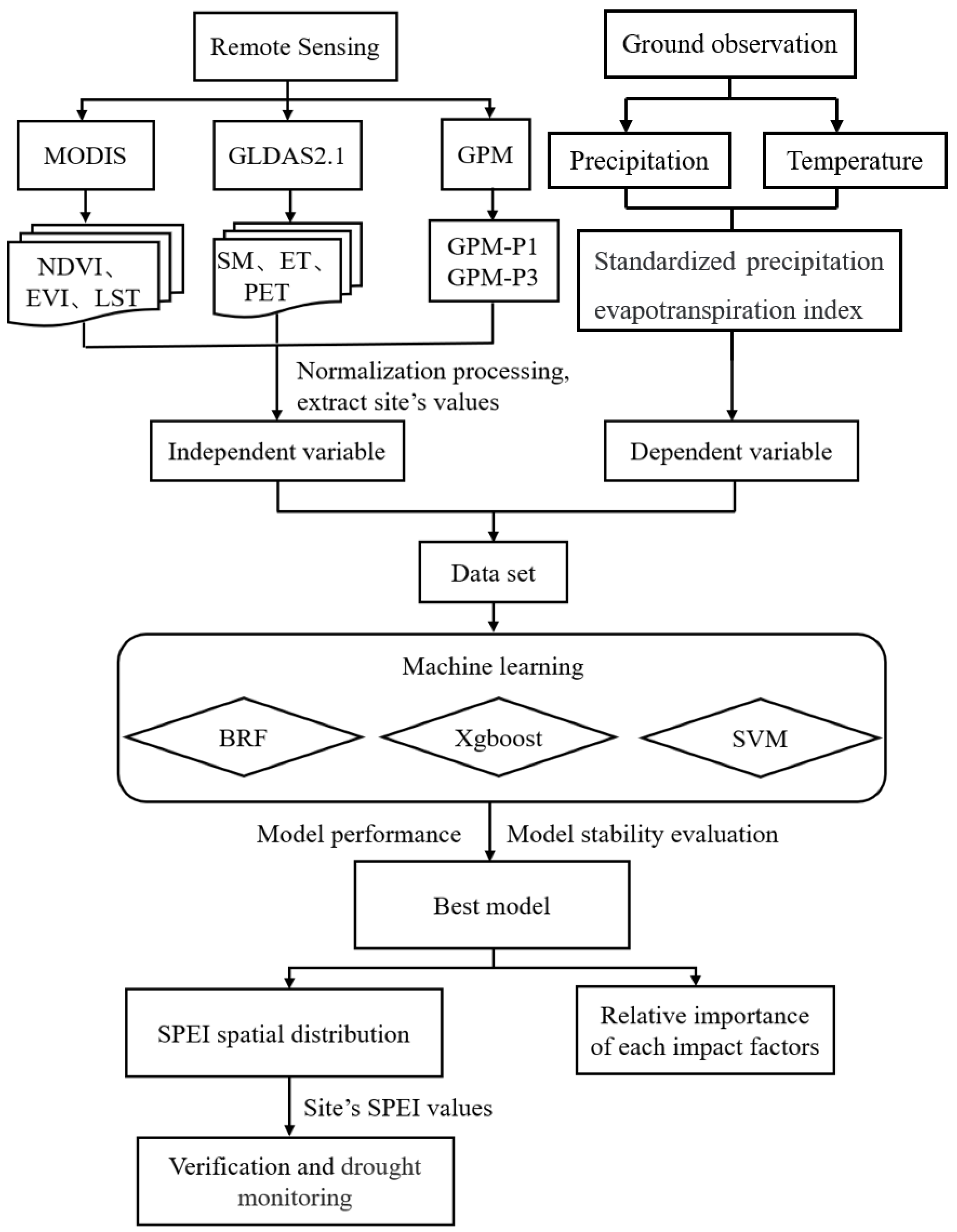
All procedures for agricultural drought assessment based on remote sensing data and model simulation data in this study are illustrated by the framework in Figure 2. Using the remote sensing drought factors calculated from multi-sensor remote sensing data, we utilized bias-corrected random forest (BRF), extreme gradient boosting (XGBoost), and support vector machines (SVM) to estimate SPEI to analyze the drought in Shandong province.
Firstly, ground-based drought index SPEI is calculated from the meteorological station data (precipitation and temperature) of Shandong province as the dependent variable of our model input. Secondly, the obtained remote sensing data are converted into images with 500 m spatial resolution employing projection coordinate conversion, resampling, band operation, and clipping through MRT, ArcGIS, and python, and through maximum/minimum values. Then, aiming at Shandong province, three adaptive machine learning approaches, namely, XGBoost, BRF, and SVM, are established to estimate agricultural drought by using remote sensing drought factors, and the best model is determined by model performance and stability evaluation in Shandong province. According to the best model, the relative importance of each influencing factor was obtained and compared with the Pearson correlation coefficient of each influencing factor with SPEI. Subsequently, the best drought monitoring model is used to create the drought spatial distribution map of Shandong province, and the SPEI spatial distribution map estimated by the model is used to analyze the drought situation of Shandong province.

2.3.2. Standardized Precipitation Evapotranspiration Index

The standardized precipitation evapotranspiration index (SPEI) has received extensive attention in the field of drought analysis [24]. An extension of the widely used SPI, SPEI considers both precipitation and temperature, which are used to calculate evapotranspiration information [63]. Therefore, unlike SPI, SPEI captures the main impact of temperature rise on water requirement.
The shorter time scale SPEIs are appropriate to monitor meteorological and agricultural drought [64], such as the one-month time scale SPEI (SPEI-1) can monitor meteorological drought, the three-month and six-month time scale SPEIs can monitor vegetation, agricultural droughts, and soil moisture dynamics [65]; while the longer time scale SPEIs are appropriate to monitor hydrological droughts [27,28]. In this study, three-month time scale of SPEI was selected.
The calculation steps of SPEI-3 are as follows [24]:
(1)
Calculation of monthly potential evapotranspiration using Thornthwaite method:
P E T = 16 K 10 T I m
In Equation (1), K is the correction factor based on latitude, T is the monthly average temperature, I is the total heating index, and m is a constant.
I = i = 1 12 T 5 1.514
m = 6.75 × 10 7 I 3 7.71 × 10 5 I 2 + 1.792 × 10 2 I + 0.49  
(2)
Calculate the difference between precipitation and potential evapotranspiration for each month.
D i = P i P E T i
In Equation (4), P i is the monthly precipitation, P E T i is the monthly potential evapotranspiration, and i denotes the month. The establishment of climate water balance accumulation at different time scale sequences is as follows:
D n k = i = 0 k 1 P n i P E T n i
In Equation (5), k is the time scale and takes the value of 3, and n is the number of calculations.
(3)
To normalize D i , first, a Log-logistic probability density function is used to build the data series:
f x = β α ( x y α ) β 1 [ 1 + ( x y ε ) ] 2
In Equation (6), α is the scale parameter and β is the shape parameter, which are the origin parameters obtained by the linear moment method, and then the cumulative probability of the D i density function is:
F x = [ 1 + ( α x y ) β ] 1  
(4)
Under normal normalization of the cumulative probability density function, the probability of exceeding a certain D i value is P = 1 F X and the probability of weighted moments are ω = 2 l n P .
When P ≤ 0.5,
S P E I = ω C 0 + C 1 ω + C 2 ω 2 1 + d 1 ω + d 2 ω 2 + d 2 ω 3
When P > 0.5,
S P E I = C 0 + C 1 ω + C 2 ω 2 1 + d 1 ω + d 2 ω 2 + d 2 ω 3  
In Equations (8) and (9), C 0 = 2.515517 , C 1 = 0.802853 , C 2 = 0.010328 , d 1 = 1.432788 , d 2 = 0.189269 , and d 3 = 0.001308 .
The monthly temperature and precipitation data from the selected weather stations were used to calculate the ground-based standard precipitation evapotranspiration index (SPEI). According to the internationally recognized criteria for classifying drought levels, SPEI is divided into five levels (Table 2).

2.3.3. Establishment of Drought Prediction Indicators

This study calculated the soil moisture condition index (SMCI) and precipitation condition index (PCI) derived from soil moisture and precipitation data, which are closely related to agricultural drought. PCI can directly respond to precipitation anomalies [66]; while SMCI can quantitatively portray the degree of wet and dry soil anomalies [67]. Temperature condition index (TCI) is calculated from MODIS LST data, which focuses on the stress of high temperature on vegetation growth, and higher values of TCI indicate more severe drought conditions [68]. Evapotranspiration represents the intensity of transpiration of plants, and the smaller the evapotranspiration, the more severe the drought [69]. The calculation formulas are shown in Table 3.

2.4. Machine Learning Approaches

2.4.1. Bias-Corrected Random Forest

Random Forest (RF) is an integrated learning algorithm that constructs multiple decision trees into a random forest by random sampling and integration methods [72]. RF first generates a number of independent trees using the sample set generated by bootstrap. With a large enough training sample, about 37% of the training data will be retained and used for subsequent out-of-bag validation [54]. For each tree in the forest, RF determines its outcome by constructing a random subset of the training set through the bootstrap method. The result of RF approaches is the means of each tree. Therefore, RF can decrease the variance and obtain more precise prediction results compared with common tree-based algorithms. However, when predicting extreme observations, it may lead to bias [55]. When the observations are small, the predictions of RF tend to overestimate; while when the observations are large, the predictions of RF tend to underestimate. In this study, we applied bias correction methods to estimate and correct for RF bias in the regression [73]. The details of this bias-correction approach is as follows:
(1)
Firstly, build the RF model by training dataset Ytrain = RF (Xtrain), where Xtrain and Ytrain represent the independent and dependent variables, respectively.
(2)
Calculate the estimated value and residual, rtrain = Ytrain − Ypredict, where rtrain represents the residual and Ypredict represents the estimated value.
(3)
Taking the residuals obtained in step (2) to be the dependent variable and training dataset in step (1) to be the independent variable, fit the random forest model, rtrain = rfres (Xtrain, Ytrain). This step is used to estimate the residual of the test dataset.
(4)
Calculate the estimated value Ytest from the RF model obtained in step (1) and the test dataset Xtest, Ytest = RF (Xtest).
(5)
Calculate the estimated residual using the rfres model in step (3), the estimated value in step 4, and the independent variables in the test dataset, rtest = rfres (Xtest, Ytest).
(6)
The estimated residual rtest is added to the estimated value Ytest for deviation correction, Ybias-correction = Ytest + rtest.

2.4.2. XGBoost

XGBoost is an extreme gradient lifting tree [56]. It efficiently realizes the gradient boosting decision tree (GDBT) algorithm disease and makes many improvements in algorithm and engineering. Compared with the traditional GBDT algorithm, XGBoost uses a random forest-like strategy for data adoption [74]. In addition, XGBoost adds a rule term to control the complexity of the model, which can only improve the generalization ability of the model and prevent over-fitting [75]. The details of XGBoost approach is as follows.
(1)
To grow a tree, constantly add new trees and continuously split features. Each time a tree is added, a new function is learned f(x) to fit the residual of the last estimation. The optimal model is constructed by minimizing the loss function: o b j t = i = 1 n l y i , y ^ i + Ω f t + C o n s t a n t .
(2)
XGBoost needs to estimate the result of a sample after it has been trained to obtain k trees. Actually, according to the characteristics of this sample, the sample will fall on one corresponding leaf node per tree, and each leaf node corresponds to a score.
Finally, XGBoost will add up the results corresponding to each tree, and it will obtain the estimate of the sample, y ^ i k = k K γ k h k x i , where K is the sum of trees, k represents the kth tree, γ k is the weight of this tree, and h k represents the estimation of this tree.

2.4.3. Support Vector Machine

Support vector machine (SVM) is one of the most widely used algorithms in machine learning. Derived from statistical learning theory, SVM algorithms are strong learners with classification and regression algorithms [76]. The purpose of SVM is to determine one or more hyperplanes to divide the samples. The segmentation principle is to maximize the interval, which is finally transformed into a convex quadratic programming problem [77]. SVM is the closest machine learning method to deep learning. Nonlinear SVM is equivalent to a two-layer neural network. If multiple kernel functions are added to nonlinear SVM, a multi-layer neural network can be simulated [78]. In this study, we implement the support vector regression model through Python’s Scikit-learn machine learning library.

2.5. Accuracy Evaluation

In this study, we enhance the machine learning approaches’ performance by identifying the parameters that affect the models’ stability through trial-and-error methods, and determine the optimal parameters for each model through cross validation. Then, BRF, XGBoost, and SVM are calibrated and validated with 80% and 20% of the dataset, respectively. The dataset is randomly sampled and divided into a training set and a test set. This step is performed 100 times to evaluate the stability of each model.
The determination coefficient ( R 2 ) and mean square error ( R M S E ) are used to evaluate the performance of the model:
R 2 = ( i = 1 n ( O i O ) ( P i P ) i = 1 n ( O i O ) i = 1 n ( P i P ) ) 2
R M S E = i = 1 n O i   P i 2 n
where n is the number of samples, O i and P i are observed and estimated values, respectively, and O and P are the mean values of the observed and estimated values. Generally, the larger R 2 and the smaller R M S E , the better the performance of the model is considered. In addition, we performed station retention cross validation for each meteorological station to identify the stability of each model in the estimation of continuous time series of drought conditions.

3. Results

3.1. Model Accuracy Comparison

This study trained BRF, XGBoost, and SVM models, respectively, using the selected influencing variables and observed SPEI-3 values. After determining the best parameters of each model by cross validation (Table 4), we compared the simulation accuracy of these algorithms, respectively. The results show that the BRF model simulates the SPEI-3 values better, and the simulated values of SPEI-3 for each site month by month from 2002 to 2020 are very close to the observed values (see Figure 3). In both training and test sets, the determination coefficient ( R 2 ) of BRF for SPEI-3 fitting are 0.96 and 0.94, and the root mean square error ( R M S E ) are 0.19 and 0.22. Compared with past studies, the bias-corrected approach significantly improves the accuracy of random forests [79]. BRF explains more than 90% of the SPEI variation with less prediction error. SVM and XGBoost models have similar performance, with R 2 of 0.72 and 0.74, and R M S E of 0.51 and 0.49, respectively.

3.2. Model Stability Evaluation

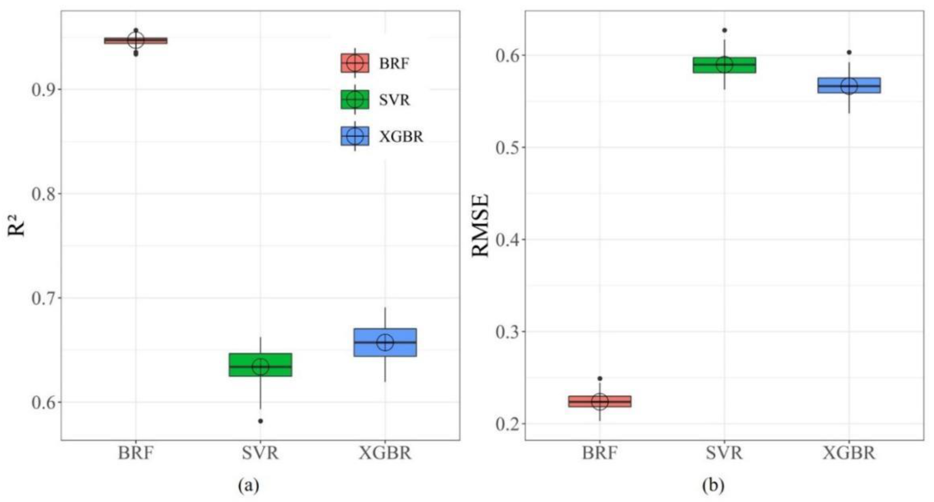
Randomly selected data sets were divided into calibration datasets and validation datasets. This step is performed 100 times to evaluate the stability of each model. The performance evaluation criteria ( R 2 and R M S E ) of the three models running 100 times are shown in Figure 4. Overall, based on these two validation measurements, the performance of the BRF model outperforms XGBoost and SVM, and the performance is satisfied. The BRF model explains more than 92% of the SPEI changes, and the estimation error is small ( R M S E < 0.25 ). In comparison, the SVM and XGBoost models have similar and lower performance.
To further evaluate the stability of the model, we conducted “leave-one-station-out” cross validation on the selected 23 meteorological stations. In this study, the meteorological stations in Heze, Huimin, Laiyang, and Yiyuan were selected for “leave-one-station-out” cross validation, which are located in the eastern, western, southern, and northern parts of Shandong, respectively. Figure 5 shows that the BRF model performs better for off-site cross validation, and the drought conditions simulated for the four stations are generally consistent with SPEI-3 calculated based on observed data. The SVM and XGBoost performed worse than the BRF model, and the simulated drought conditions at the four sites differed significantly from the SPEI-3 calculated based on the observed data.

3.3. Analyzing the Relative Importance of Drought-Influencing Factors Using the BRF Model

The BRF model can produce a measure of relative importance based on the impact of each predictor on the outcome [80]. The results in Table 5 show that, Pre_3 has the highest relative importance with 55.17%; the relative importance of Pre_1 is 8.61%, indicating that precipitation is the most important variable affecting drought. Because we used SPEI on a three-month time scale, SPEI-3 is related to agricultural drought [25,27]; therefore, cumulative precipitation is more important for monitoring agricultural drought. The relative importance of soil moisture was 10.2%, which indicated the significance of SM in simulating agricultural drought. The relative importance of other influencing factors was low for drought. Generally, the response of vegetation to drought is lagging, and the impact of drought on vegetation tends to occur after a few months, so this leads to a low relative importance of the vegetation indices NDVI and EVI.
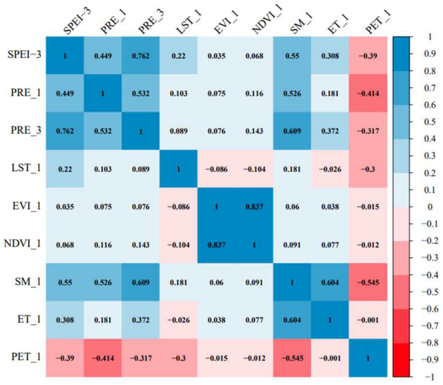
We analyzed the correlation between SPEI-3 and drought impact factors, which are shown in Figure 6. The correlation analysis indicated that significant relationships existed among each factor and SPEI-3, with the highest correlation of 0.762 between PRE_3 and SPEI-3. The correlations of SM and PRE_1 with SPEI-3 were 0.55 and 0.449, respectively. The correlation between vegetation index and SPEI-3 was low. These were consistent with the results of our analysis of the relative importance of the factors obtained from the BRF model.

3.4. Simulation of Drought by Spatial Distribution of SPEI-3 in Typical Years

In this study, the average value of SPEI-3 from 23 meteorological stations during the study period was used to obtain the change process of SPEI-3 from 2002 to 2020. It can be seen from Figure 7 that the drought was relatively serious and lasted for a long time in 2002–2003, 2006–2007, and 2010–2011. Severe drought occurred in autumn of 2002 and 2006, winter of 2010, and spring of 2011. Drought occurred frequently but with low intensity from 2012 to 2019. From 2003–2004 and 2007–2008, the whole province was in the wet period. However, the duration and intensity of drought in other periods have no obvious laws. For the period marked by the dashed box in Figure 7, SPEI-3 shows higher drought intensity and longer drought duration, which was selected as typical drought years.
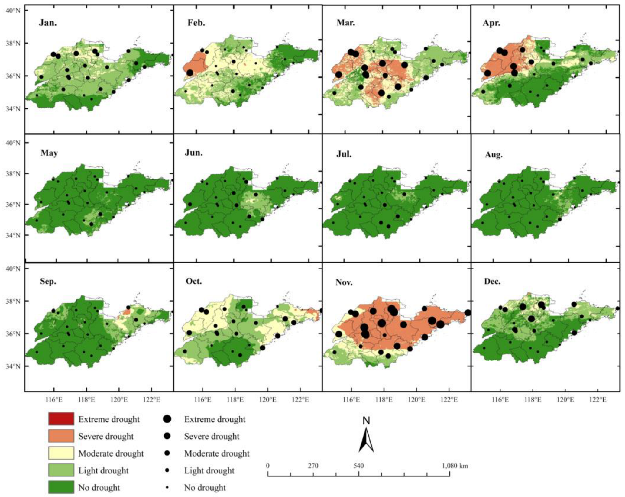
Using SPEI-3 spatial distribution data and station observation of SPEI-3 data to evaluate the accuracy of SPEI-3 spatial distribution for drought monitoring, the drought year data of 2002, 2006, and 2011 were selected and the results are shown in Figure 8, Figure 9 and Figure 10. According to the drought grade distribution of meteorological stations in Figure 8, it can be seen that all meteorological stations in northwestern Shandong province experienced severe drought in February, while the rest of the meteorological stations experienced moderate and light drought; most meteorological stations in western Shandong province experienced severe drought in March, which is basically consistent with the SPEI drought grade distribution map constructed by BRF. From April to June, as the rain belt moved southwest, the drought conditions eased and the province’s meteorological stations were not in drought. Due to the high temperature and low rainfall in Shandong during the summer of 2002, most meteorological stations in the province, except for the eastern peninsula, experienced severe drought from August to October, and the drought class distribution map constructed for this experiment monitored severe drought during this period. Ren and Zhan also monitored the drought conditions in Shandong province from February–March and August–October 2002, and the drought was more severe from August–October [19]. Drought in Shandong during this period is related to the El Niño phenomenon and the duration of no effective precipitation [81]. In November, the drought disappeared as the high temperature subsided and was supplemented by effective precipitation.
From Figure 9, it can be seen that in January 2006, most meteorological stations in the province were in light drought and some meteorological stations in the northwest were in moderate drought. In February, the meteorological stations in the eastern peninsula and the southeast coast were in no drought or light drought, while some meteorological stations in the western part of Shandong were in moderate as well as severe drought. In March, the drought conditions in the central and northwest intensified, and meteorological stations in the region detected moderate and severe drought. In April, with the increase in precipitation, the drought conditions in the central part were relieved, but the meteorological stations in the northwest were still in severe drought. With the arrival of the rainy season, the drought in Shandong province eased. Severe and extreme drought was detected at most meteorological stations in Shandong province in November and moderate drought was detected at some meteorological stations. In addition, it can be seen from Figure 10 that all meteorological stations in Shandong province were in severe and extreme drought in January 2011, except for some meteorological stations in the eastern peninsula, which was caused by the low precipitation from December 2010 to January 2011. The drought conditions monitored at each meteorological station are generally consistent with the SPEI drought class distribution map. Yao et al. also monitored the overall drought period in Shandong province from February–March and November 2006, and December 2010–January 2011 [82]. Overall, the SPEI-3 spatial distribution map simulated by the BRF model can more accurately monitor the drought conditions in Shandong province and is generally consistent with the drought periods identified by historical drought studies.

4. Discussion

Data-driven models have proven to be effective in previous drought monitoring [29,40]. This study, based on machine learning with multi-source remote sensing drought factors fitting SPEI, also obtained effective drought monitoring results. In particular, the BRF model is better than the SVM and XGBoost models in reproducing ground SPEI (Figure 4 and Figure 5), which is quantified by large R 2 and small prediction error R M S E . However, the result of Alizadeh and Nikoo showed that the MLP model significantly improved the SPI prediction in Iran compared with other machine learning models, which is inconsistent with the results of this research [40]. This may be the result of differences in study area, data sources, and model and model parameters, as well as input and output settings. This study determined the best parameters of each model through cross validation. However, in different regions, the performance of the model was not invariable when dealing with data from different sources. In this study, the excellent performance of the BRF model may be due to its reduced sensitivity to over fitting and handling the possible hierarchical and nonlinear relationship between SPEI and various remote sensing drought factors. Furthermore, the bias correction random forest [73] outperforms the original random forest [29].
In addition, the relative importance of each drought factor was obtained according to the BRF model (Table 5), and precipitation on a three-month time scale (GPM-P3) had the highest relative importance of 55.17%. The relative importance of precipitation on a one-month time scale (GPM-P1) is 8.61%. Consistent with Yang, precipitation is the most significant factor affecting drought [83]. In addition, the relative importance of GPM-P3 is much higher than that of GPM-P1 because the SPEI chose a three-month time scale, indicating that GPM-P3 has the greatest impact on agricultural drought. Feng also demonstrated that the precipitation of a three-month time scale has the greatest impact on agricultural drought, and its relative importance exceeds 0.55 in the two clusters [25]. Soil moisture (SM), with a relative importance of 10.2%, plays an important role in simulating SPEI-3 [84,85]. The results were generally consistent with the Pearson correlation coefficients of each drought factor with SPEI-3 (Figure 6). GPM-P3 has the highest correlation with SPEI-3 at 0.762. The correlation coefficient between SM and SPEI-3 is 0.55. In addition, the correlation between SM and GPM-P3 (0.609) was higher than that with GPM-P1 (0.526), indicating that soil moisture was more influenced by cumulative precipitation.
In this study, we accurately predicted SPEI-3 in unmeasured areas based on the BRF model and remote sensing data. Firstly, we used the BRF model to simulate SPEI-3 in unmeasured areas, rather than taking the relative importance obtained after model training as the weight to build a comprehensive drought index. Constructing a composite drought index based on relative importance as weights often allows monitoring drought. However, due to the different study areas, the drought classification of the composite drought index does not follow the unique criteria. The effect of drought monitoring is different from the actual distribution of the ground drought index.

5. Conclusions

In this study, three machine learning methods (BRF, SVM, and XGBoost) and various drought impact factors were used to estimate SPEI-3 in Shandong, China. Taking the monthly dataset based on surface climate data as a reference, the performance of SPEI predicted by the model was evaluated. The BRF model successfully generated the spatial distribution map of SPEI-3. Therefore, the method in this study can also be used in other areas with limited observation data and covered by remote sensing satellites, providing spatial distribution of drought severity. Due to the complex causes of drought, altitude and vegetation cover type also have an impact on drought. These factors need to be considered in future studies to increase the precision of the models for more accurate monitoring of drought conditions. In addition, the BRF model also has some limitations, such as the tendency to underestimate the severity of drought when predicting extreme drought. Future research should consider better machine learning models and other drought-causing factors to improve the performance of the models in assessing extreme droughts.

Author Contributions

Y.Z., data curation, investigation, software, code, writing—original draft; J.Z., conceptualization, funding acquisition, supervision; writing—review; Y.B., software, visualization, writing—review; S.Z., code, visualization, writing—review; S.Y., visualization, writing—review; M.H., A.M.S. and L.N., writing—review. All authors have read and agreed to the published version of the manuscript.

Funding

This work was jointly supported by the National Natural Science Foundation of China (No. 41871253, No. 42071425), the CAS Strategic Priority Research Program (No. XDA19030402), Shandong Natural Science Foundation of China (No. ZR2017ZB0422, No. ZR2020QE281), and “Taishan Scholar” Project of Shandong Province (No. TSXZ201712).

Institutional Review Board Statement

Not applicable.

Informed Consent Statement

Not applicable.

Data Availability Statement

Not applicable.

Conflicts of Interest

The authors declare no conflict of interest.

References

  1. Ali, S.; Tong, D.M.; Xu, Z.T.; Henchiri, M.; Wilson, K.; Shi, S.Q.; Zhang, J.H. Characterization of Drought Monitoring Events through Modis-and Trmm-Based Dsi and Tvdi over South Asia During 2001–2017. Environ. Sci. Pollut. Res. 2019, 26, 33568–33581. [Google Scholar] [CrossRef] [PubMed]
  2. Quiring, S.M.; Papakryiakou, T.N. An Evaluation of Agricultural Drought Indices for the Canadian Prairies. Agric. For. Meteorol. 2003, 118, 49–62. [Google Scholar] [CrossRef]
  3. Wei, W.; Pang, S.F.; Wang, X.F.; Zhou, L.; Xie, B.B.; Zhou, J.J.; Li, C.H. Temperature Vegetation Precipitation Dryness Index (Tvpdi)-Based Dryness-Wetness Monitoring in China. Remote Sens. Environ. 2020, 248, 111957. [Google Scholar] [CrossRef]
  4. Yao, N.; Li, Y.; Lei, T.J.; Peng, L.L. Drought Evolution, Severity and Trends in Mainland China over 1961–2013. Sci. Total Environ. 2018, 616, 73–89. [Google Scholar] [CrossRef]
  5. Trenberth, K.E.; Dai, A.; Van Der Schrier, G.; Jones, P.D.; Barichivich, J.; Briffa, K.R.; Sheffield, J. Global Warming and Changes in Drought. Nat. Clim. Change 2014, 4, 17. [Google Scholar] [CrossRef]
  6. Dai, A.G. Erratum: Drought under Global Warming: A Review. Wiley Interdiscip. Rev.-Clim. Chang. 2012, 3, 617. [Google Scholar] [CrossRef] [Green Version]
  7. Vicente-Serrano, S.M.; Quiring, S.M.; Pena-Gallardo, M.; Yuan, S.S.; Dominguez-Castro, F. A Review of Environmental Droughts: Increased Risk under Global Warming? Earth-Sci. Rev. 2020, 201, 102953. [Google Scholar] [CrossRef]
  8. Daryanto, S.; Wang, L.X.; Jacinthe, P.A. Global Synthesis of Drought Effects on Food Legume Production. PLoS ONE 2015, 10, e0127401. [Google Scholar] [CrossRef] [Green Version]
  9. Daryanto, S.; Wang, L.X.; Jacinthe, P.A. Global Synthesis of Drought Effects on Maize and Wheat Production. PLoS ONE 2016, 11, e0156362. [Google Scholar] [CrossRef] [Green Version]
  10. Loon, V.; Anne, F. Hydrological Drought Explained. Wiley Interdiscip. Rev. Water 2015, 2, 359–392. [Google Scholar] [CrossRef]
  11. Allen, C.D.; Macalady, A.K.; Chenchouni, H.; Bachelet, D.; Mcdowell, N.; Vennetier, M.; Kitzberger, T.; Rigling, A.; Breshears, D.D.; Hogg, E.H.; et al. A Global Overview of Drought and Heat-Induced Tree Mortality Reveals Emerging Climate Change Risks for Forests. For. Ecol. Manag. 2010, 259, 660–684. [Google Scholar] [CrossRef] [Green Version]
  12. Ciais, P.; Reichstein, M.; Viovy, N.; Granier, A.; Ogee, J.; Allard, V.; Aubinet, M.; Buchmann, N.; Bernhofer, C.; Carrara, A.; et al. Europe-Wide Reduction in Primary Productivity Caused by the Heat and Drought in 2003. Nature 2005, 437, 529–533. [Google Scholar] [CrossRef] [PubMed]
  13. Zhao, M.S.; Running, S.W. Drought-Induced Reduction in Global Terrestrial Net Primary Production from 2000 through 2009. Science 2010, 329, 940–943. [Google Scholar] [CrossRef] [Green Version]
  14. Aadhar, S.; Mishra, V. High-Resolution near Real-Time Drought Monitoring in South Asia. Sci. Data 2017, 4, 170145. [Google Scholar] [CrossRef] [PubMed] [Green Version]
  15. He, B.; Wu, J.J.; Lu, A.F.; Cui, X.F.; Zhou, L.; Liu, M.; Zhao, L. Quantitative Assessment and Spatial Characteristic Analysis of Agricultural Drought Risk in China. Nat. Hazards 2013, 66, 155–166. [Google Scholar] [CrossRef]
  16. Mottaleb, K.A.; Gumma, M.K.; Mishra, A.K.; Mohanty, S. Quantifying Production Losses Due to Drought and Submergence of Rainfed Rice at the Household Level Using Remotely Sensed Modis Data. Agric. Syst. 2015, 137, 227–235. [Google Scholar] [CrossRef]
  17. Prodhan, F.A.; Zhang, J.H.; Yao, F.M.; Shi, L.M.; Sharma, T.P.P.; Zhang, D.; Cao, D.; Zheng, M.X.; Ahmed, N.; Mohana, H.P. Deep Learning for Monitoring Agricultural Drought in South Asia Using Remote Sensing Data. Remote Sens. 2021, 13, 1715. [Google Scholar] [CrossRef]
  18. Yang, X.; Li, D. Temporal and Spatial Evolution Characteristics of Strong Drought Events in North and Northeast China. Arid Land Geogr. 2019, 42, 810–821. [Google Scholar]
  19. Ren, J.; Zhang, T. Evolution Characteristics of Drought and Flood in Shandong Province in Recent 45years Based on Standardized Precipitation Index. Res. Soil Water Conserv. 2021, 28, 149. [Google Scholar]
  20. Zhang, J.; Mu, Q.Z.; Huang, J.X. Assessing the Remotely Sensed Drought Severity Index for Agricultural Drought Monitoring and Impact Analysis in North China. Ecol. Indic. 2016, 63, 296–309. [Google Scholar] [CrossRef]
  21. Yan, H.; Wan, Y.; Yan, X.; Xie, Y. A Study of the Temporal and Spatial Features of Dryness & Wetness Last 500-Year Period in China. J. Yunnan Univ. (Nat. Sci.) 2004, 26, 139–143. [Google Scholar]
  22. Zhang, Y.; Wang, C.; Zhang, J. Analysis of the Spatial and Temporal Characteristics of Drought in the North China Plain Based on Standardized Precipitation Evapotranspiration Index. Acta Ecol. Sin. 2015, 35, 7097–7107. [Google Scholar]
  23. Mckee, T.B.; Doesken, N.J.; Kleist, J. The Relationship of Drought Frequency and Duration to Time Scales. In Proceedings of the 8th Conference on Applied Climatology, Anaheim, CA, USA, 17–22 January 1993; pp. 179–184. [Google Scholar]
  24. Vicente-Serrano, S.M.; Begueria, S.; Lopez-Moreno, J.I. A Multiscalar Drought Index Sensitive to Global Warming: The Standardized Precipitation Evapotranspiration Index. J. Clim. 2010, 23, 1696–1718. [Google Scholar] [CrossRef] [Green Version]
  25. Feng, P.Y.; Wang, B.; Liu, D.L.; Yu, Q. Machine Learning-Based Integration of Remotely-Sensed Drought Factors Can Improve the Estimation of Agricultural Drought in South-Eastern Australia. Agric. Syst. 2019, 173, 303–316. [Google Scholar] [CrossRef]
  26. Rhee, J.; Im, J.; Carbone, G.J. Monitoring Agricultural Drought for Arid and Humid Regions Using Multi-Sensor Remote Sensing Data. Remote Sens. Environ. 2010, 114, 2875–2887. [Google Scholar] [CrossRef]
  27. Liu, Q.; Zhang, J.H.; Zhang, H.R.; Yao, F.M.; Bai, Y.; Zhang, S.; Meng, X.L.; Liu, Q. Evaluating the Performance of Eight Drought Indices for Capturing Soil Moisture Dynamics in Various Vegetation Regions over China. Sci. Total Environ. 2021, 789, 147803. [Google Scholar] [CrossRef]
  28. Yao, N.; Li, Y.; Liu, Q.Z.; Zhang, S.Y.; Chen, X.G.; Ji, Y.D.; Liu, F.G.; Pulatov, A.; Feng, P.Y. Response of Wheat and Maize Growth-Yields to Meteorological and Agricultural Droughts Based on Standardized Precipitation Evapotranspiration Indexes and Soil Moisture Deficit Indexes. Agric. Water Manag. 2022, 266, 107566. [Google Scholar] [CrossRef]
  29. Park, S.; Im, J.; Jang, E.; Rhee, J. Drought Assessment and Monitoring through Blending of Multi-Sensor Indices Using Machine Learning Approaches for Different Climate Regions. Agric. For. Meteorol. 2016, 216, 157–169. [Google Scholar] [CrossRef]
  30. Swain, S.; Wardlow, B.D.; Narumalani, S.; Tadesse, T.; Callahan, K. Assessment of Vegetation Response to Drought in Nebraska Using Terra-Modis Land Surface Temperature and Normalized Difference Vegetation Index. Giscience Remote Sens. 2011, 48, 432–455. [Google Scholar] [CrossRef]
  31. Ali, S.; Henchiri, M.; Yao, F.M.; Zhang, J.H. Analysis of Vegetation Dynamics, Drought in Relation with Climate over South Asia from 1990 to 2011. Environ. Sci. Pollut. Res. 2019, 26, 11470–11481. [Google Scholar] [CrossRef]
  32. Shi, S.Q.; Yao, F.M.; Zhang, J.H.; Yang, S.S. Evaluation of Temperature Vegetation Dryness Index on Drought Monitoring over Eurasia. IEEE Access 2020, 8, 30050–30059. [Google Scholar] [CrossRef]
  33. Wu, D.; Qu, J.J.; Hao, X.J. Agricultural Drought Monitoring Using Modis-Based Drought Indices over the USA Corn Belt. Int. J. Remote Sens. 2015, 36, 5403–5425. [Google Scholar] [CrossRef]
  34. Souza, A.; Neto, A.R.; Rossato, L.; Alvala, R.C.S.; Souza, L.L. Use of Smos L3 Soil Moisture Data: Validation and Drought Assessment for Pernambuco State, Northeast Brazil. Remote Sens. 2018, 10, 1314. [Google Scholar] [CrossRef] [Green Version]
  35. Bai, Y.; Gao, J.; Zhang, B. Monitoring of Crops Growth Based on Ndvi and Evi. Trans. Chin. Soc. Agric. Mach. 2019, 50, 153–161. [Google Scholar]
  36. Gu, Y.X.; Brown, J.F.; Verdin, J.P.; Wardlow, B. A Five-Year Analysis of Modis Ndvi and Ndwi for Grassland Drought Assessment over the Central Great Plains of the United States. Geophys. Res. Lett. 2007, 34. [Google Scholar] [CrossRef]
  37. Lei, Q.; Zhang, X.; Wang, X.; He, X.; Shang, C. Responses of Vegetation Index to Meteorological Drought in Dongting Lake Basin Based on Modis-Evi and Ci. Resour. Environ. Yangtze Basin 2019, 28, 981–993. [Google Scholar]
  38. Wang, K.Y.; Li, T.J.; Wei, J.H. Exploring Drought Conditions in the Three River Headwaters Region from 2002 to 2011 Using Multiple Drought Indices. Water 2019, 11, 190. [Google Scholar] [CrossRef] [Green Version]
  39. Liu, H.; Liu, R.; Liu, S. Review of Drought Monitoring by Remote Sensing. J. Geo-Inf. Sci. 2012, 14, 232–239. [Google Scholar] [CrossRef]
  40. Alizadeh, M.R.; Nikoo, M.R. A Fusion-Based Methodology for Meteorological Drought Estimation Using Remote Sensing Data. Remote Sens. Environ. 2018, 211, 229–247. [Google Scholar] [CrossRef]
  41. Han, P.; Wang, P.X.; Zhang, S.Y.; Zhu, D.H. Drought Forecasting Based on the Remote Sensing Data Using Arima Models. Math. Comput. Model. 2010, 51, 1398–1403. [Google Scholar] [CrossRef]
  42. Mishra, A.K.; Singh, V.P. Drought Modeling—A Review. J. Hydrol. 2011, 403, 157–175. [Google Scholar] [CrossRef]
  43. Wanders, N.; Wood, E.F. Improved Sub-Seasonal Meteorological Forecast Skill Using Weighted Multi-Model Ensemble Simulations. Environ. Res. Lett. 2016, 11, 094007. [Google Scholar] [CrossRef]
  44. Morid, S.; Smakhtin, V.; Bagherzadeh, K. Drought Forecasting Using Artificial Neural Networks and Time Series of Drought Indices. Int. J. Climatol. 2007, 27, 2103–2111. [Google Scholar] [CrossRef]
  45. Wang, Q.J.; Schepen, A.; Robertson, D.E. Merging Seasonal Rainfall Forecasts from Multiple Statistical Models through Bayesian Model Averaging. J. Clim. 2012, 25, 5524–5537. [Google Scholar] [CrossRef]
  46. Abbot, J.; Marohasy, J. Input Selection and Optimisation for Monthly Rainfall Forecasting in Queensland, Australia, Using Artificial Neural Networks. Atmos. Res. 2014, 138, 166–178. [Google Scholar] [CrossRef]
  47. Hao, Z.C.; Singh, V.P.; Xia, Y.L. Seasonal Drought Prediction: Advances, Challenges, and Future Prospects. Rev. Geophys. 2018, 56, 108–141. [Google Scholar] [CrossRef]
  48. Barua, S.; Ng, A.W.M.; Perera, B.J.C. Artificial Neural Network-Based Drought Forecasting Using a Nonlinear Aggregated Drought Index. J. Hydrol. Eng. 2012, 17, 1408–1413. [Google Scholar] [CrossRef]
  49. Dikshit, A.; Pradhan, B.; Alamri, A.M. Temporal Hydrological Drought Index Forecasting for New South Wales, Australia Using Machine Learning Approaches. Atmosphere 2020, 11, 585. [Google Scholar] [CrossRef]
  50. Khan, N.; Sachindra, D.A.; Shahid, S.; Ahmed, K.; Shiru, M.S.; Nawaz, N. Prediction of Droughts over Pakistan Using Machine Learning Algorithms. Adv. Water Resour. 2020, 139, 103562. [Google Scholar] [CrossRef]
  51. Mishra, A.K.; Desai, V.R. Drought Forecasting Using Feed-Forward Recursive Neural Network. Ecol. Model. 2006, 198, 127–138. [Google Scholar] [CrossRef]
  52. Belayneh, A.; Adamowski, J.; Khalil, B.; Ozga-Zielinski, B. Long-Term Spi Drought Forecasting in the Awash River Basin in Ethiopia Using Wavelet Neural Network and Wavelet Support Vector Regression Models. J. Hydrol. 2014, 508, 418–429. [Google Scholar] [CrossRef]
  53. Guzman, S.M.; Paz, J.O.; Tagert, M.L.M.; Mercer, A.E.; Pote, J.W. An Integrated Svr and Crop Model to Estimate the Impacts of Irrigation on Daily Groundwater Levels. Agric. Syst. 2018, 159, 248–259. [Google Scholar] [CrossRef]
  54. Cutler, D.R.; Edwards, T.C.; Beard, K.H.; Cutler, A.; Hess, K.T.; Gibson, J.; Lawler, J.J. Random Forests for Classification in Ecology. Ecology 2007, 88, 2783–2792. [Google Scholar] [CrossRef]
  55. Song, J. Bias Corrections for Random Forest in Regression Using Residual Rotation. J. Korean Stat. Soc. 2015, 44, 321–326. [Google Scholar] [CrossRef]
  56. Chen, T.Q.; Guestrin, C.; Assoc Comp, M. Xgboost: A Scalable Tree Boosting System. In Proceedings of the 22nd ACM SIGKDD International Conference on Knowledge Discovery and Data Mining (KDD), San Francisco, CA, USA, 13–17 August 2016. [Google Scholar]
  57. Chen, Y.; Niu, J.Q.; Chen, G.Q.; Wang, J.; Cao, S.L.; Publishing, I.O.P. Precipitation Sequence Analysis of Representative Stations in Shandong Province from 1956 to 2016. In Proceedings of the 6th International Conference on Energy Materials and Environment Engineering (ICEMEE), Zhangjiajie, China, 24–26 April 2020. [Google Scholar]
  58. Li, H.; Wang, W. Climate Characteristics of Seasonal Drought for Crops Growth in Shandong. J. Arid Land Resour. Environ. 2015, 29, 191–196. [Google Scholar]
  59. Li, F.; Yang, X. Changes and Driving Force of Grain Production in Shandong Province During 1999–2014. Acta Agric. Zhejiangensis 2016, 28, 535–542. [Google Scholar]
  60. Han, H.Z.; Bai, J.J.; Yan, J.W.; Yang, H.Y.; Ma, G. A Combined Drought Monitoring Index Based on Multi-Sensor Remote Sensing Data and Machine Learning. Geocarto Int. 2021, 36, 1161–1177. [Google Scholar] [CrossRef]
  61. Shen, R.P.; Huang, A.Q.; Li, B.L.; Guo, J. Construction of a Drought Monitoring Model Using Deep Learning Based on Multi-Source Remote Sensing Data. Int. J. Appl. Earth Obs. Geoinf. 2019, 79, 48–57. [Google Scholar] [CrossRef]
  62. Tapiador, F.J.; Turk, F.J.; Petersen, W.; Hou, A.Y.; Garcia-Ortega, E.; Machado, L.A.; Angelis, C.F.; Salio, P.; Kidd, C.; Huffman, G.J.; et al. Global Precipitation Measurement: Methods, Datasets and Applications. Atmos. Res. 2012, 104, 70–97. [Google Scholar] [CrossRef]
  63. Zhao, J.; Yan, D.H.; Yang, Z.Y.; Hu, Y.; Weng, B.S.; Gong, B.Y. Improvement and Adaptability Evaluation of Standardized Precipitation Evapotranspiration Index. Acta Phys. Sin. 2015, 64, 049202. [Google Scholar] [CrossRef]
  64. Almeida-Naunay, A.F.; Villeta, M.; Quemada, M.; Tarquis, A.M. Assessment of Drought Indexes on Different Time Scales: A Case in Semiarid Mediterranean Grasslands. Remote Sens. 2022, 14, 565. [Google Scholar] [CrossRef]
  65. Wen, J.; Zhang, X.; Wang, Y.; Wang, W. Effects of Drought in Multi-Time Scale on Wheat Crop in Eastern Agricultural Region of Qinghai Province. J. Irrig. Drain. 2016, 35, 92–97. [Google Scholar]
  66. Javed, T.; Zhang, J.H.; Bhattarai, N.; Sha, Z.; Rashid, S.; Yun, B.; Ahmad, S.; Henchiri, M.; Kamran, M. Drought Characterization across Agricultural Regions of China Using Standardized Precipitation and Vegetation Water Supply Indices. J. Clean. Prod. 2021, 313, 127866. [Google Scholar] [CrossRef]
  67. Zhang, J.H.; Zhou, Z.M.; Yao, F.M.; Yang, L.M.; Hao, C. Validating the Modified Perpendicular Drought Index in the North China Region Using in Situ Soil Moisture Measurement. IEEE Geosci. Remote Sens. Lett. 2015, 12, 542–546. [Google Scholar] [CrossRef]
  68. Wu, L. Classification of Drought Grades Based on Temperature Vegetation Drought Index Using the Modis Data. Res. Soil Water Conserv. 2017, 24, 130–135. [Google Scholar]
  69. Wang, Y.P.; Wang, S.; Zhao, W.W.; Liu, Y.X. The Increasing Contribution of Potential Evapotranspiration to Severe Droughts in the Yellow River Basin. J. Hydrol. 2022, 605, 127310. [Google Scholar] [CrossRef]
  70. Seiler, R.A.; Kogan, F.; Sullivan, J. Avhrr-Based Vegetation and Temperature Condition Indices for Drought Detection in Argentina. Adv. Space Res. 1998, 21, 481–484. [Google Scholar] [CrossRef]
  71. Kogan, F.N. Application of Vegetation Index and Brightness Temperature for Drought Detection. Adv. Space Res. 1995, 15, 91–100. [Google Scholar] [CrossRef]
  72. Ishwaran, H.; Malley, J.D. Synthetic Learning Machines. Biodata Min. 2014, 7, 28. [Google Scholar] [CrossRef] [Green Version]
  73. Zhang, G.Y.; Lu, Y. Bias-Corrected Random Forests in Regression. J. Appl. Stat. 2012, 39, 151–160. [Google Scholar] [CrossRef]
  74. Li, H.; Zhu, Y. Xgboost Algorithm Optimization Based on Gradient Distribution Harmonized Strategy. J. Comput. Appl. 2020, 40, 1633–1637. [Google Scholar]
  75. Chen, J.X.; Zhao, F.; Sun, Y.G.; Yin, Y.L. Improved Xgboost Model Based on Genetic Algorithm. Int. J. Comput. Appl. Technol. 2020, 62, 240–245. [Google Scholar] [CrossRef]
  76. Corinna, C.; Vladimir, V. Support-Vector Networks. Mach. Learn. 1995, 20, 273–297. [Google Scholar]
  77. Haitao, L.I.; Haiyan, G.U.; Bing, Z.; Lianru, G. Research on Hyperspectral Remote Sensing Image Classification Based on Mnf and Svm. Remote Sens. Inf. 2007, 5, 12–15. [Google Scholar]
  78. Mountrakis, G.; Im, J.; Ogole, C. Support Vector Machines in Remote Sensing: A Review. Isprs J. Photogramm. Remote Sens. 2011, 66, 247–259. [Google Scholar] [CrossRef]
  79. Shen, R.; Guo, J.; Zhang, J.; Li, L. Construction of a Drought Monitoring Model Using the Random Forest Based Remote Sensing. J. Geo-Inf. Sci. 2017, 19, 125–133. [Google Scholar]
  80. Were, K.; Bui, D.T.; Dick, O.B.; Singh, B.R. A Comparative Assessment of Support Vector Regression, Artificial Neural Networks, and Random Forests for Predicting and Mapping Soil Organic Carbon Stocks across an Afromontane Landscape. Ecol. Indic. 2015, 52, 394–403. [Google Scholar] [CrossRef]
  81. Xu, Z.; Han, M. Spatio-Temporal Distribution Characteristics of Drought in Shandong Province and It Relationship with Enso. Chin. J. Eco-Agric. 2018, 26, 1236–1248. [Google Scholar]
  82. Yao, T.; Zhao, Q.; Li, X.Y.; Shen, Z.T.; Ran, P.Y.; Wu, W. Spatiotemporal Variations of Multi-Scale Drought in Shandong Province from 1961 to 2017. Water Supply 2021, 21, 525–541. [Google Scholar] [CrossRef]
  83. Yang, M.X.; Mou, Y.L.; Meng, Y.R.; Liu, S.; Peng, C.H.; Zhou, X.L. Modeling the Effects of Precipitation and Temperature Patterns on Agricultural Drought in China from 1949 to 2015. Sci. Total Environ. 2020, 711, 135139. [Google Scholar] [CrossRef]
  84. Seneviratne, S.I.; Corti, T.; Davin, E.L.; Hirschi, M.; Jaeger, E.B.; Lehner, I.; Orlowsky, B.; Teuling, A.J. Investigating Soil Moisture-Climate Interactions in a Changing Climate: A Review. Earth-Sci. Rev. 2010, 99, 125–161. [Google Scholar] [CrossRef]
  85. Sims, A.P.; Niyogi, D.D.S.; Raman, S. Adopting Drought Indices for Estimating Soil Moisture: A North Carolina Case Study. Geophys. Res. Lett. 2002, 29, 24-1–24-4. [Google Scholar] [CrossRef]
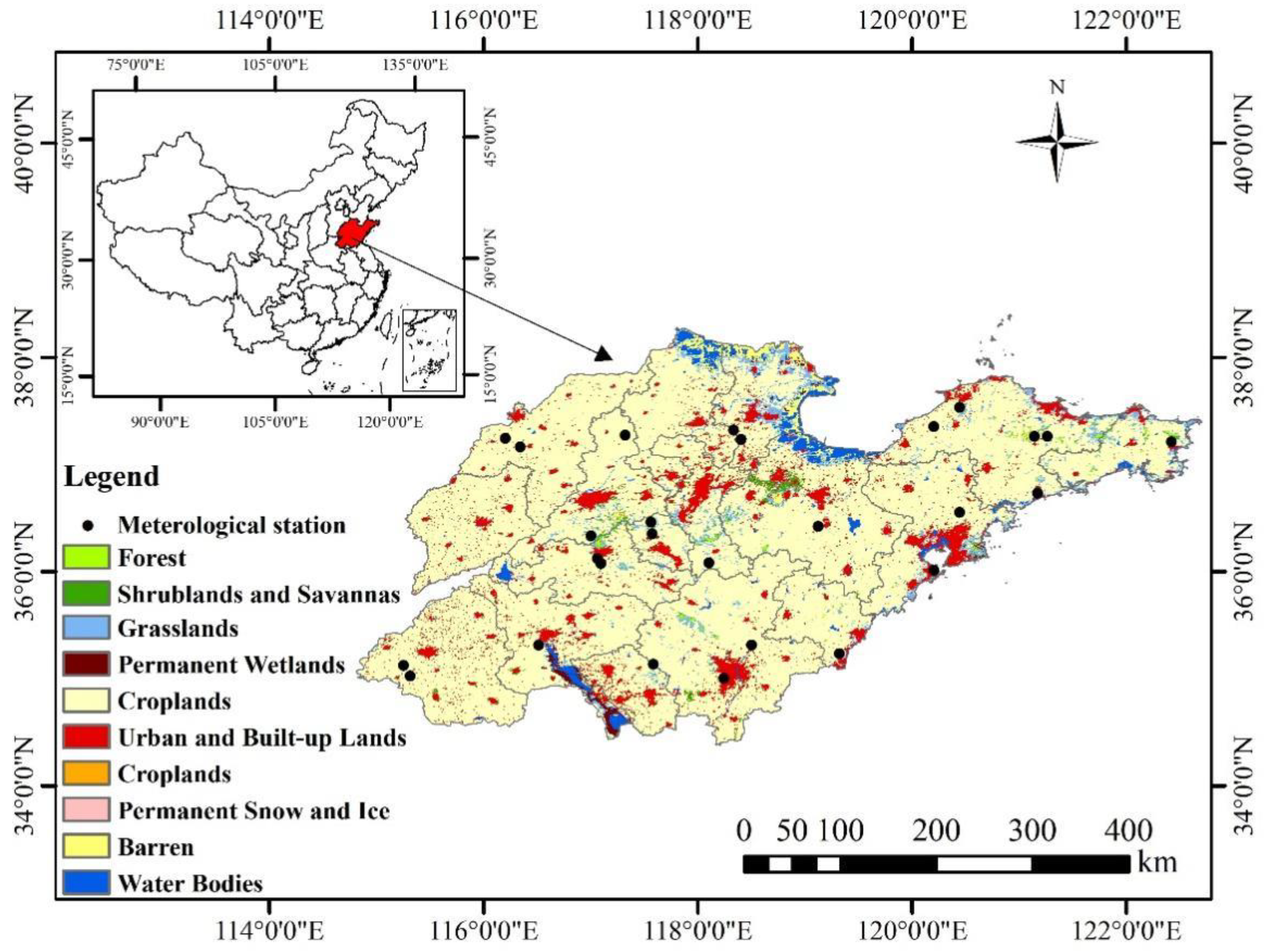
Figure 1. Location and land cover types of the study area in Shandong province.
Remotesensing 14 06398 g001
Figure 2. Workflow of this study.
Remotesensing 14 06398 g002
Figure 3. Scatterplot of model predictions vs. observations. (a,c,e) is the performance of BRF, SVM, and XGBoost on the training set. (b,d,f) is the performance of BRF, SVM, and XGBoost on the test set. “**” represents the significance level of the experiment is greater than 0.99.
Remotesensing 14 06398 g003
Figure 4. Boxplots of model performance measurements ((a). coefficient of determination and (b). root mean squared error) for prediction of SPEI.
Remotesensing 14 06398 g004
Figure 5. Comparation among SPEI−3 calculated from observations and forecasted by BRF, XGBoost, and SVM approaches at four stations in Shandong province, China.
Remotesensing 14 06398 g005
Figure 6. Pearson correlation coefficients of SPEI-3 with drought impact factors. The “1” and “3” suffixes following the variable name represent the average of one-month and three-month time scales.
Remotesensing 14 06398 g006
Figure 7. The change of SPEI−3 in Shandong province from 2002 to 2020.
Remotesensing 14 06398 g007
Figure 8. SPEI-3 spatial distribution simulated by the BRF model and the site’s drought distribution in a drought year (2002).
Remotesensing 14 06398 g008
Figure 9. SPEI-3 spatial distribution simulated by the BRF model and the site’s drought distribution in a drought year (2006).
Remotesensing 14 06398 g009
Figure 10. SPEI-3 spatial distribution simulated by the BRF model and the site’s drought distribution in a drought year (2011).
Remotesensing 14 06398 g010
Table 1. Remote sensing data used in this study.
DataTemporal ResolutionSpatial ResolutionTime SpanSource
Precipitation1-month0.1°2001~2020GPM
NDVI1-month1 km2002~2020MODIS
EVI1-month1 km2002~2020MODIS
LST8-day1 km2002~2020MODIS
Soil moisture1-month0.25°2002~2020GLDAS
Evapotranspiration1-month0.25°2002~2020GLDAS
Potential evapotranspiration1-month0.25°2002~2020GLDAS
Table 2. SPEI-3 classification criteria for grading drought.
GradeDrought ConditionSPEI
INo drought−0.5 < SPEI
IILight drought−1.0 < SPEI ≤ −0.5
IIIModerate drought−1.5 < SPEI ≤ −1.0
IVSevere drought−2.0 < SPEI ≤ −1.5
VExtreme droughtSPEI ≤ −2.0
Table 3. Normalization formula for calculating seven types of impact factors for each grid.
Drought IndexFormulaReference
PCI GPM i GPM min / GPM max GPM min [26]
SMCI SM i SM min / SM max SM min [70]
TCI LST max LST i / LST max LST min [71]
VCI NDVI i NDVI min / NDVI max NDVI min [71]
Scaled EVI EVI i EVI min / EVI max EVI min [71]
Scaled ET ET i ET min / ET max ET min [33]
Scaled PET PET i EVI min / PET max PET min [33]
Note: i represents the month; max and min represent the maximum and minimum values of the corresponding grid of the impact factor from 2002 to 2020.
Table 4. The detailed list of parameters with their values used for BRF, XGBoost, and SVM.
ModelParameters
BRFRF1: criterion = ‘mse’, n_estimators = 800, max_depth = 5, min_samples_leaf = 4, max_features = ‘auto’, random_state = 0, bootstrap = TrueRF2: criterion = ‘mse’, n_estimators = 1000, max_depth = 5, min_samples_leaf = 4, max_features = ‘auto’, random_state = 0, bootstrap = True
XGBoostn_estimators = 100, learning_rate = 0.04, max_depth = 5, gamma = 0.5, consample_bytree = 1, consample_bylevel = 1, subsample = 0.52, booster = ‘gbtree’, objective = ‘reg:squarederror’, reg_alpha = 0.7, reg_lambda = 0
SVMkernel = ‘rbf’, gamma = 0.85, C = 50, tol = 0.01, cache_size = 5000, degree = 3, coef0 = 2.5
Table 5. Relative importance of factors to drought assessment.
Impact FactorsRelative Importance (%)
One-month timescale precipitation, Pre_18.61
Three-month timescale precipitation, Pre_355.17
Land surface temperature, LST7.39
Enhanced vegetation index, EVI3.54
Normalized difference vegetation index, NDVI3.3
Soil moisture, SM10.2
Evapotranspiration, ET7.3
Potential evapotranspiration, PET4.49
Publisher’s Note: MDPI stays neutral with regard to jurisdictional claims in published maps and institutional affiliations.