
Activity of Okgye Limestone Mine in South Korea Observed by InSAR Coherence and PSInSAR Techniques


Abstract

1. Introduction
2. Materials
2.1. Study Area
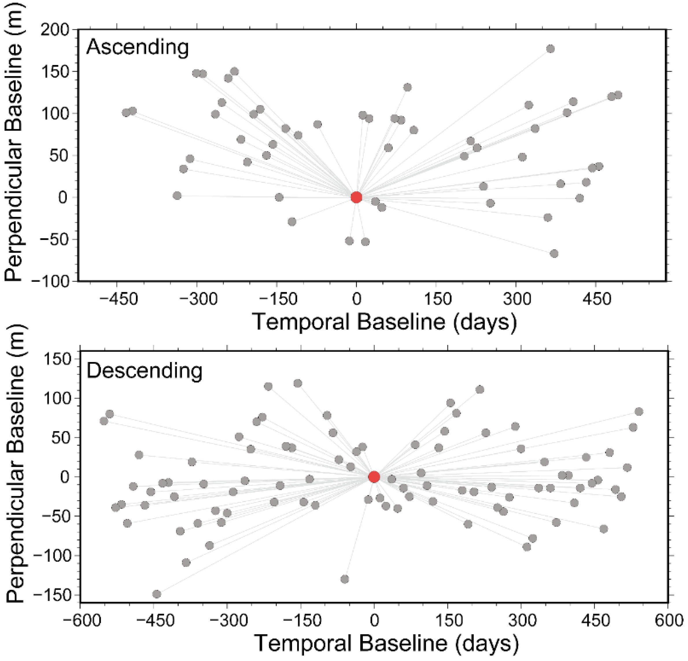
2.2. Dataset
3. Methods
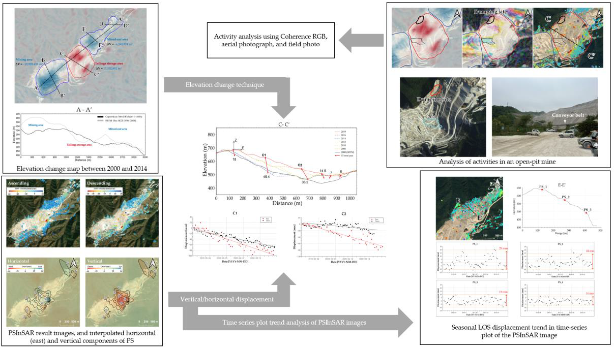
3.1. Elevation and Volume Change
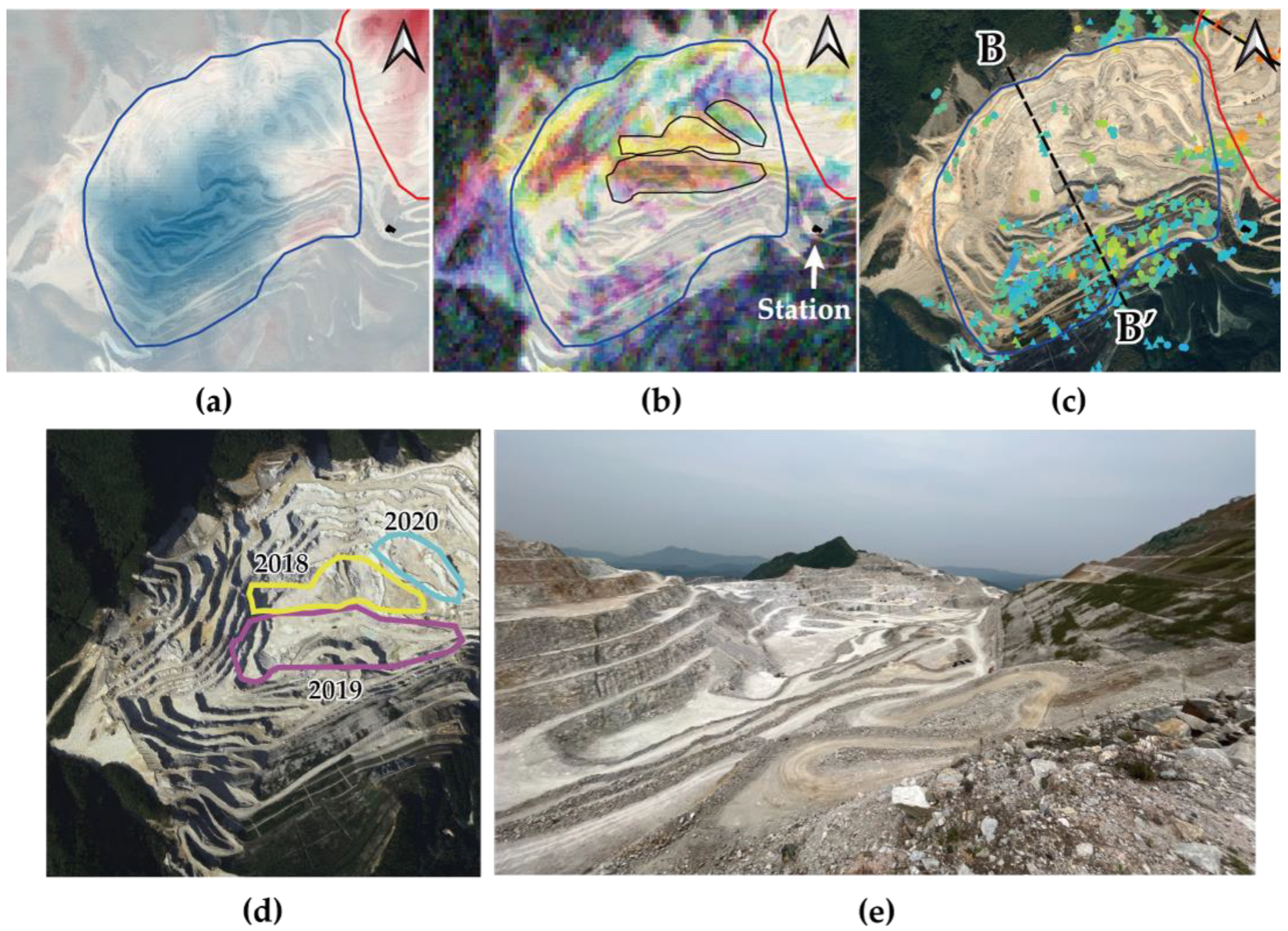
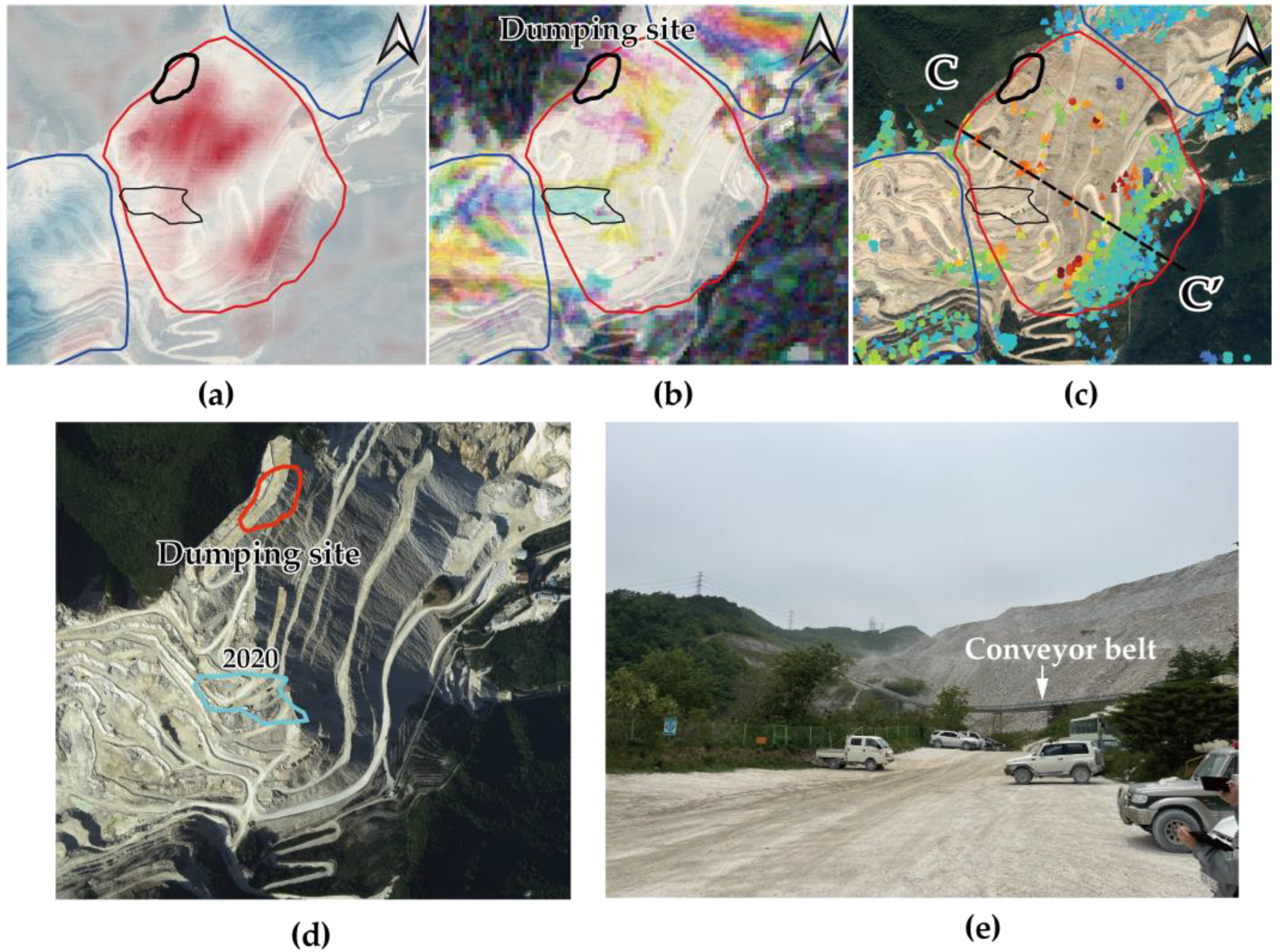
3.2. Coherence and RGB Compositing
3.3. PSInSAR Using Both Ascending and Descending Orbits
4. Results
4.1. Elevation and Volume Change during 2010 to 2014
4.2. The Mining Area
4.3. The Tailings Storage Area
4.4. The Mined-Out Area
4.5. Thermal Expansion of Limestone and Iron
5. Discussion
6. Conclusions
Author Contributions
Funding
Data Availability Statement
Conflicts of Interest
References
- Hu, H.; Fernández-Steeger, T.M.; Dong, M.; Azzam, R. Deformation Monitoring and Modeling Based on LiDAR Data for Slope Stability Assessment. In Proceedings of the 19. Tagung Für Ingenieurgeologie, Munich, Germany, 13–16 March 2013. [Google Scholar]
- Lee, S.; Jang, Y. Stability Assesment of the Slope at the Disposal Site of Waste Rock in Limestone Mine. Tunn. Undergr. Space 2010, 20, 475–490. [Google Scholar]
- Carlà, T.; Intrieri, E.; Raspini, F.; Bardi, F.; Farina, P.; Ferretti, A.; Colombo, D.; Novali, F.; Casagli, N. Perspectives on the Prediction of Catastrophic Slope Failures from Satellite InSAR. Sci. Rep. 2019, 9, 1–9. [Google Scholar] [CrossRef] [PubMed]
- Blikra, L.H.; Fasani, G.B.; Esposito, C.; Lenti, L.; Martino, S.; Pecci, M.; Mugnozza, G.S.; Kalenchuk, K.S.; Hutchinson, D.J.; Diederichs, M. 26 the Aknes Rockslide, Norway. In Landslides: Types, Mechanisms and Modeling; Cambridge University Press: Cambridge, UK, 2012; p. 323. [Google Scholar]
- Michoud, C.; Bazin, S.; Blikra, L.H.; Derron, M.; Jaboyedoff, M. Experiences from Site-Specific Landslide Early Warning Systems. Nat. Hazards Earth Syst. Sci. 2013, 13, 2659–2673. [Google Scholar] [CrossRef]
- United Nations Office on Disaster Risk Reduction. United Nations System for Disaster Risk Reduction (UNISDR), U. UNISDR Terminology on Disaster Risk Reduction; United Nations Office on Disaster Risk Reduction: Geneva, Switzerland, 2009. [Google Scholar]
- Ferretti, A.; Monti-Guarnieri, A.V.; Prati, C.M.; Rocca, F.; Massonnet, D. InSAR Principles: Guideline for SAR Interferometry Processing and Interpretation; ESA Publication: Noordwijk, The Netherlands, 2007. [Google Scholar]
- Carlà, T.; Farina, P.; Intrieri, E.; Ketizmen, H.; Casagli, N. Integration of Ground-Based Radar and Satellite InSAR Data for the Analysis of an Unexpected Slope Failure in an Open-Pit Mine. Eng. Geol. 2018, 235, 39–52. [Google Scholar] [CrossRef]
- Casagli, N.; Catani, F.; Del Ventisette, C.; Luzi, G. Monitoring, Prediction, and Early Warning using Ground-Based Radar Interferometry. Landslides 2010, 7, 291–301. [Google Scholar] [CrossRef]
- Casagli, N.; Frodella, W.; Morelli, S.; Tofani, V.; Ciampalini, A.; Intrieri, E.; Raspini, F.; Rossi, G.; Tanteri, L.; Lu, P. Spaceborne, UAV and Ground-Based Remote Sensing Techniques for Landslide Mapping, Monitoring and Early Warning. Geoenvironmental Disasters 2017, 4, 1–23. [Google Scholar] [CrossRef]
- Hanssen, R.F. Radar Interferometry: Data Interpretation and Error Analysis; Springer Science & Business Media: Berlin, Germany, 2001. [Google Scholar] [CrossRef]
- Ferretti, A.; Prati, C.; Rocca, F. Permanent Scatterers in SAR Interferometry. IEEE Trans. Geosci. Remote Sens. 2001, 39, 8–20. [Google Scholar] [CrossRef]
- Lee, H.; Liu, J.G. Analysis of Topographic Decorrelation in SAR Interferometry using Ratio Coherence Imagery. IEEE Trans. Geosci. Remote Sens. 2001, 39, 223–232. [Google Scholar] [CrossRef]
- Han, H.; Kim, Y.; Jin, H.; Lee, H. Analysis of Annual Variability of Landfast Sea Ice Near Jangbogo Antarctic Station using InSAR Coherence Images. Korean J. Remote Sens. 2015, 31, 501–512. [Google Scholar] [CrossRef]
- Moon, J.; Lee, H. Analysis of Activity in an Open-Pit Mine by using InSAR Coherence-Based Normalized Difference Activity Index. Remote Sens. 2021, 13, 1861. [Google Scholar] [CrossRef]
- Paradella, W.R.; Ferretti, A.; Mura, J.C.; Colombo, D.; Gama, F.F.; Tamburini, A.; Santos, A.R.; Novali, F.; Galo, M.; Camargo, P.O. Mapping Surface Deformation in Open Pit Iron Mines of Carajás Province (Amazon Region) using an Integrated SAR Analysis. Eng. Geol. 2015, 193, 61–78. [Google Scholar] [CrossRef]
- Hartwig, M.E.; Paradella, W.R.; Mura, J.C. Detection and Monitoring of Surface Motions in Active Open Pit Iron Mine in the Amazon Region, using Persistent Scatterer Interferometry with TerraSAR-X Satellite Data. Remote Sens. 2013, 5, 4719–4734. [Google Scholar] [CrossRef]
- Hallacement. Available online: https://www.hallacement.co.kr/company/siteguide (accessed on 1 August 2022).
- Kim, M.; Kim, K. Seokbyeongsan Area (Limestone) Detailed Geological Survey Report; Korea Mine Rehabilitation and Mineral Resources Corporation: Wonju-si, Republic of Korea, 2020. [Google Scholar]
- Lee, H.J.; Kim, S.Y.; Jang, B.J.; Kim, K.D. Analysis and Selection of Ganwon-do Open-Pit Mine Monitoring Target Area. In Proceedings of the 2014 Conference on the Geospatial Information, Incheon, Korea, November 2014; pp. 91–92. [Google Scholar]
- Kim, K.; Joo, P.; Kim, H. A Study of Rehabilitation for Limestone Quarry Near Baekdu Daegan Mountain System (1)-in Case Study for Hydroseeding Experiment on Okke Quarry. J. Korean Soc. Environ. Restor. Technol. 2011, 14, 55–66. [Google Scholar] [CrossRef]
- Kim, K.; Kim, H. A Study of Rehabilitation for Limestone Quarry Near the Baekdudaegan Mountains (2)-in Case Study for Planting Seedlings Experiment on Okke Quarry. J. Korean Soc. Environ. Restor. Technol. 2012, 15, 117–125. [Google Scholar] [CrossRef][Green Version]
- Earthexplorer. Available online: https://earthexplorer.usgs.gov (accessed on 26 January 2022).
- CREODIAS Finder. Available online: https://finder.creodias.eu (accessed on 26 January 2022).
- National Geographic Information Service. Available online: https://map.ngii.go.kr/ms/map/NlipMap.do (accessed on 21 August 2022).
- Copernicus Open Access Hub. Available online: https://scihub.copernicus.eu/dhus/#/home (accessed on 26 January 2022).
- ASF Data Search Vertex. Available online: https://search.asf.alaska.edu/#/?dataset=AVNIR (accessed on 21 September 2022).
- Jaber, W.A.; Floricioiu, D.; Rott, H.; Eineder, M. Surface Elevation Changes of Glaciers Derived from SRTM and TanDEM-X DEM Differences. In Proceedings of the 2013 IEEE International Geoscience and Remote Sensing Symposium-IGARSS, Melbourne, VIC, Australia, 21–26 July 2013; pp. 1893–1896. [Google Scholar] [CrossRef]
- Parwata, I.N.S.; Nakashima, S.; Shimizu, N.; Osawa, T. Effect of Digital Elevation Models on Monitoring Slope Displacements in Open-Pit Mine by Differential Interferometry Synthetic Aperture Radar. J. Rock Mech. Geotech. Eng. 2020, 12, 1001–1013. [Google Scholar] [CrossRef]
- Hooper, A.; Segall, P.; Zebker, H. Persistent Scatterer Interferometric Synthetic Aperture Radar for Crustal Deformation Analysis, with Application to Volcán Alcedo, Galápagos. J. Geophys. Res. Solid Earth 2007, 112. [Google Scholar] [CrossRef]
- Wang, Q.; Yu, W.; Xu, B.; Wei, G. Assessing the use of GACOS Products for SBAS-INSAR Deformation Monitoring: A Case in Southern California. Sensors 2019, 19, 3894. [Google Scholar] [CrossRef]
- Höser, T. Analysing the Capabilities and Limitations of InSAR Using Sentinel-1 Data for Landslide Detection and Monitoring. Master’s Thesis, University of Bonn, Bonn, Germany, 2018. [Google Scholar]
- Cian, F.; Blasco, J.M.D.; Carrera, L. Sentinel-1 for Monitoring Land Subsidence of Coastal Cities in Africa using PSInSAR: A Methodology Based on the Integration of SNAP and StaMPS. Geosciences 2019, 9, 124. [Google Scholar] [CrossRef]
- Delgado Blasco, J.M.; Foumelis, M.; Stewart, C.; Hooper, A. Measuring Urban Subsidence in the Rome Metropolitan Area (Italy) with Sentinel-1 SNAP-StaMPS Persistent Scatterer Interferometry. Remote Sens. 2019, 11, 129. [Google Scholar] [CrossRef]
- Li, Z.; Muller, J.; Cross, P.; Fielding, E.J. Interferometric Synthetic Aperture Radar (InSAR) Atmospheric Correction: GPS, Moderate Resolution Imaging Spectroradiometer (MODIS), and InSAR Integration. J. Geophys. Res. Solid Earth 2005, 110. [Google Scholar] [CrossRef]
- Bekaert, D.; Walters, R.J.; Wright, T.J.; Hooper, A.J.; Parker, D.J. Statistical Comparison of InSAR Tropospheric Correction Techniques. Remote Sens. Environ. 2015, 170, 40–47. [Google Scholar] [CrossRef]
- Bekaert, D.; Hooper, A.; Wright, T.J. A Spatially Variable Power Law Tropospheric Correction Technique for InSAR Data. J. Geophys. Res. Solid Earth 2015, 120, 1345–1356. [Google Scholar] [CrossRef]
- Yu, C.; Penna, N.T.; Li, Z. Generation of Real-time Mode High-resolution Water Vapor Fields from GPS Observations. J. Geophys. Res. Atmos. 2017, 122, 2008–2025. [Google Scholar] [CrossRef]
- GIS-Blog. Available online: https://gitlab.com/Rexthor/gis-blog/-/blob/master/StaMPS/2-4_StaMPS-steps.md (accessed on 21 September 2022).
- Tang, W.; Motagh, M.; Zhan, W. Monitoring Active Open-Pit Mine Stability in the Rhenish Coalfields of Germany using a Coherence-Based SBAS Method. Int. J. Appl. Earth Obs. Geoinf. 2020, 93, 102217. [Google Scholar] [CrossRef]
- Jin, L.; Funning, G.J. Testing the Inference of Creep on the Northern Rodgers Creek Fault, California, using Ascending and Descending Persistent Scatterer InSAR Data. J. Geophys. Res. Solid Earth 2017, 122, 2373–2389. [Google Scholar] [CrossRef]
- Fuhrmann, T.; Garthwaite, M.C. Resolving Three-Dimensional Surface Motion with InSAR: Constraints from Multi-Geometry Data Fusion. Remote Sens. 2019, 11, 241. [Google Scholar] [CrossRef]
- Crosetto, M.; Monserrat, O.; Cuevas-González, M.; Devanthéry, N.; Luzi, G.; Crippa, B. Measuring Thermal Expansion using X-Band Persistent Scatterer Interferometry. ISPRS J. Photogramm. Remote Sens. 2015, 100, 84–91. [Google Scholar] [CrossRef]
- Lazecky, M.; Perissin, D.; Bakon, M.; de Sousa, J.M.; Hlavacova, I.; Real, N. Potential of Satellite InSAR Techniques for Monitoring of Bridge Deformations. In Proceedings of the 2015 Joint Urban Remote Sensing Event (JURSE), Lausanne, Switzerland, 30 March–1 April 2015; pp. 1–4. [Google Scholar] [CrossRef]
- Cohen-Waeber, J.F. Spatiotemporal Patterns of Seasonality in Landslide Deformation from InSAR and GPS; University of California: Berkeley, CA, USA, 2018. [Google Scholar]
- Kim, K. Use of Low-Grade Limestone for Cement Industry as Concrete Aggregate. Mag. RCR 2016, 11, 20–23. [Google Scholar] [CrossRef]


| Technique | Satellite | Pass | Orbit | Frame | Date (YYYY/MM/DD~YYYY/MM/DD) | Number of Data |
|---|---|---|---|---|---|---|
| Coherence | Sentinel-1B | Descending | 61 | 470 | 2018/01/03~2020/12/30 | 91 |
| PSInSAR | Sentinel-1B | Descending | 61 | 470 | 2019/01/10~2020/12/30 | 66 |
| Sentinel-1A/B | Ascending | 54 | 117 | 2019/01/04~2020/12/24 | 41 |
| Parameter | Scla_Deramp | Unwrap_Gold_n_Win | Unwrap_Grid_Size | Unwrap_Time_Win | Scn_Time_Win |
|---|---|---|---|---|---|
| Default | ‘N’ | 32 | 200 | 730 | 365 |
| Used | ‘Y’ | 8 | 10 | 24 | 50 |
| Type | Mining Area | Tailings Storage Area | Mined-Out Area | Total |
|---|---|---|---|---|
| Hard Rock (R) [m3] | −19,959,439 | 11,972,024 * | −6,240,931 | −14,228,346 |
| Cavity (c) [m3] | −8,554,045 * | 5,130,868 * | −2,674,685 * | −6,097,862 |
| Dumped Material (R + c) [m3] | −28,513,484 * | 17,102,892 | −8,915,616 * | −20,326,208 |
| Mass [million ton] | −54.89 ** | 32.92 ** | −17.16 ** | −39.13 |
| Type | Limestone PS1 | Limestone PS2 | Limestone PS3 | Transmission Tower |
|---|---|---|---|---|
| Length (L) [m] | 394 | 242 | 90 | 145 |
| LOS displacement () [mm] | 29 | 24 | 18 | 54 |
| Thermal Expansion Coefficient () [] | 1.9 | 2.5 | 5.0 | 9.3 |
| of Pure Material [] | 4~8 (Limestone) | 11 (Iron) | ||
Publisher’s Note: MDPI stays neutral with regard to jurisdictional claims in published maps and institutional affiliations. |
© 2022 by the authors. Licensee MDPI, Basel, Switzerland. This article is an open access article distributed under the terms and conditions of the Creative Commons Attribution (CC BY) license (https://creativecommons.org/licenses/by/4.0/).
Share and Cite
Lee, H.; Moon, J.; Lee, H. Activity of Okgye Limestone Mine in South Korea Observed by InSAR Coherence and PSInSAR Techniques. Remote Sens. 2022, 14, 6261. https://doi.org/10.3390/rs14246261
Lee H, Moon J, Lee H. Activity of Okgye Limestone Mine in South Korea Observed by InSAR Coherence and PSInSAR Techniques. Remote Sensing. 2022; 14(24):6261. https://doi.org/10.3390/rs14246261
Chicago/Turabian StyleLee, Hoseung, Jihyun Moon, and Hoonyol Lee. 2022. "Activity of Okgye Limestone Mine in South Korea Observed by InSAR Coherence and PSInSAR Techniques" Remote Sensing 14, no. 24: 6261. https://doi.org/10.3390/rs14246261
APA StyleLee, H., Moon, J., & Lee, H. (2022). Activity of Okgye Limestone Mine in South Korea Observed by InSAR Coherence and PSInSAR Techniques. Remote Sensing, 14(24), 6261. https://doi.org/10.3390/rs14246261