Abstract
LiDAR technology has been widely used to characterize structural parameters of forest ecosystems, which in turn are valuable information for forest monitoring. GEDI is a spaceborne LiDAR system specifically designed to measure vegetation’s vertical structure, and it has been acquiring waveforms on a global scale since April 2019. In particular, canopy height is an important descriptor of forest ecosystems, as it allows for quantifying biomass and other inventory information. This paper analyzes the accuracy of canopy height estimates from GEDI data over tropical forests in French Guiana and Gabon. The influence of various signal acquisition and processing parameters is assessed to highlight how they impact the estimation of canopy heights. Canopy height models derived from airborne LiDAR data are used as reference heights. Several linear and non-linear approaches are tested given the richness of the available GEDI information. The results show that the use of regression models built on multiple GEDI metrics allows for reaching improved accuracies compared to a direct estimation from a single GEDI height metric. In a notable way, random forest improves the canopy height estimation accuracy by almost 80% (in terms of RMSE) compared to the use of rh_95 as a direct proxy of canopy height. Additionally, convolutional neural networks calibrated on GEDI waveforms exhibit similar results to the ones of other regression models. Beam type as well as beam sensitivity, which are related to laser penetration, appear as parameters of major influence on the data derived from GEDI waveforms and used as input for canopy height estimation. Therefore, we recommend the use of only power and high-sensitivity beams when sufficient data are available. Finally, we note that regression models trained on reference data can be transferred across study sites that share identical environmental conditions.
1. Introduction
Tropical forest ecosystems play a major role in natural balances as they contribute to the global carbon storage. They act as natural carbon dioxide sinks and contain more than 40% of the terrestrial carbon stock [1]. In order to understand their capability for carbon sequestration, standing aboveground biomass (AGB) is a fundamental factor that allows for quantifying the amount of carbon dioxide that they can absorb. AGB is defined as the quantity of living vegetation above the soil, including stem, stump, branches, bark, seed and foliage. Several studies have defined allometric relationships linking the measurable characteristics of a forest to its AGB levels [2,3]. In particular, canopy height is a key parameter for biomass quantification, as most allometric equations rely on canopy heights for AGB estimation [4]. Many authors demonstrated that the inclusion of canopy heights in AGB prediction models allows for reducing the estimation errors and for reaching improved accuracies [5,6].
To estimate canopy heights at regional and global scales, Earth observation data has proven to be a valuable source of information, especially since it provides informative indicators over large areas that cannot be studied otherwise [7]. For the characterization of forest vertical structures, light detection and ranging (LiDAR) is the most suited technology, as it measures the geometrical structure of the environment by emitting laser pulses and by retrieving the return signals resulting from the interaction between the laser and the forest individual elements. Discrete return (DR) LiDAR systems record multiple echoes for each emitted pulse and provide 3D point clouds describing the vegetation structure from the top of the canopy to the ground. The statistical analysis of the 3D point clouds’ spatial distribution then allows for the extraction of forest biophysical variables through different approaches [8,9]. Full waveform (FW) systems record the full profiles of the return signals by sampling them in fixed time intervals. The resulting received waveforms consist of geolocated one-dimensional temporal signals describing the vertical structure of the vegetation at given geolocations, from which diverse forest parameters can then be extracted [10]. In another perspective, optical systems are used to study state parameters of forest stands since they only measure the reflectance from the canopy’s upper layer and cannot penetrate through the vegetation. For example, the radiometric data retrieved from optical sensors allows for characterizing stand compositions and tree species by analyzing the spectral information contained in the images [11,12]. In contrast, other active sensors such as synthetic aperture radar (SAR) use lower frequency electromagnetic waves than those used by LiDARs but still present advantages for the study of forest ecosystems. Because of their longer wavelengths, radar signals tend to penetrate the forest canopy and reach the ground. SAR polarimetry and tomography techniques can provide information on the vertical structure of forested areas. In particular, starting from 2023, the European Space Agency (ESA) BIOMASS mission will collect P-band SAR data and deliver global estimates of forest biomass and height [13]. In the context of canopy height estimation, optical and radar data can provide complementary information and enrich prediction models [14,15] even though LiDAR remains the most adapted technology to derive accurate structural indicators of forest ecosystems. However, unlike SAR, spaceborne LiDARs do not provide measurements with sufficient spatial density for accurate mapping of tree height and forest biomass. Thus, in the future, the complementarity between optical, radar and LiDAR data will be exploited to produce canopy height and forest AGB maps.
Airborne and spaceborne LiDARs are the two main systems that are of interest for the description of forest vertical structures. The main advantage of airborne sensors is the very high resolutions at which they operate (availability of a high number of returned points over a given surface), but in return, it implies high financial costs that restrict their usage to limited areas. On the contrary, spaceborne LiDAR data are freely accessible and provide information with global coverage. Their counterparts are a low density of available information (spatial coverage of about 4% of the Earth’s surface for the latest system) [16] as well as their high operational altitudes that make them more sensitive to unfavorable environmental conditions [17,18]. There are currently two operating spaceborne systems providing LiDAR data globally: the Advanced Topographic Laser Altimeter System (ATLAS) onboard the Ice, Cloud, and land Elevation Satellite (IceSAT-2) and the Global Ecosystem Dynamics Investigation (GEDI) attached to the International Space Station (ISS). These systems emit laser pulses that pass through the atmosphere and interact with the objects on the Earth surface, thus producing a return signal by backscattering. They measure the profiles of the return signals by sampling them in fixed time intervals (e.g., 1 ns in the case of GEDI, which is equivalent to a 15 cm sampling distance) and differ by the technology they use. ATLAS is a photon counting system equipped with a 532 nm laser producing six distinct beams. Its main scientific objectives are, on one hand, to finely characterize ice sheets in the context of recent sea level change and, on the other hand, to collect measurements over forests to facilitate canopy height determination as a basis for estimating global biomass and biomass change [19]. GEDI is a FW LiDAR sensor that was specifically designed to measure the vertical structure of the Earth’s forest ecosystems [16]. It has been acquiring data since April 2019 through the use of three identical 1064 nm lasers. One laser is divided into two beams of half power (coverage beams) while the other two remain at full power (power beams). These coverage and power beams are slightly dithered to finally give eight parallel tracks of observations across a 4.2 km swath on the ground (four coverage beams and four power beams). Each laser emits 242 pulses per second and illuminates a 25 m circular footprint on the Earth’s surface over which the vertical structure of the vegetation is measured through the recording and processing of received waveforms.
The characterization of forest parameters from GEDI data is particularly challenging in tropical biomes since these ecosystems are usually very dense and developed. The main factor impacting canopy height estimates is the signal’s capability to penetrate through the vegetation to accurately describe the vertical structure of the vegetation all the way from the top-of-canopy to the ground [20]. Additionally, the extraction of relevant descriptive metrics from the GEDI-received waveforms requires the use of extraction algorithms that can be tuned differently depending on factors such as the forest type or the study site’s location. Given the characteristics of the GEDI system and its processing chain, the objective of this paper is to assess the influence of various signal acquisition and processing parameters on the estimation of canopy heights over tropical forests in French Guiana and Gabon. GEDI-derived heights are compared to reference values from a canopy height model (CHM) derived from airborne LiDAR (ALS) data. Firstly, a comparative analysis of the performances of GEDI’s predefined extraction algorithms is performed to understand how the algorithm tuning parameters can impact the waveform metrics used for canopy heights retrieval. Through this analysis, we aim at identifying the most adapted algorithm setting group for the processing of GEDI data in a tropical context characterized by dense forests and high AGB values. Then, in the same spirit, the influence of GEDI’s beam type is studied to evaluate which laser configuration is most suited for the estimation of canopy heights. Coverage and power beams correspond to different energy levels for the emitted laser pulses, and therefore, the beam type has a major influence on the resulting return waveforms. Other signal parameters such as beam sensitivity and signal-to-noise ratio (SNR) are also taken into account to better evaluate how the signal physical parameters can affect the information contained in the received waveforms. Our goal is to analyze and understand the link between the accuracy of canopy height estimates and the aforementioned signal parameters that are linked to the laser penetration through dense vegetation. Finally, we test several regression approaches based on GEDI data to assess how the accuracies of canopy height prediction models can be improved through the use of multiple metrics derived from GEDI waveforms. A stepwise multilinear regression (called hereafter “stepwise regression for canopy height estimation”, SRH) and a random forest (RF) are implemented to take advantage of the information contained in GEDI metrics. Moreover, to overcome the possible issues related to the generation of relevant metrics from the GEDI data [21], we test a metric-free approach through the use of convolutional neural networks (CNN) built directly onto the GEDI waveforms. The viability of model transferability across study sites is also analyzed to understand how reference data can be valued to build general canopy height estimators. Given the results of this comparative analysis, we aim at providing GEDI users with key inputs and recommendations on how to take advantage of their data depending on the specific configurations of their studies. GEDI information is quite rich and can be used in diverse manners to derive structural indicators describing forest ecosystems.
2. Materials and Methods
2.1. Study Areas
The study was conducted on four areas of interest over equatorial eco-climatic zones, specifically, two sites in French Guiana (South America) and two sites in Gabon (Africa).
Regarding French Guiana, the first site, the Nouragues Ecological Research Station, is located 120 km south of Cayenne (Figure 1a). It is a protected natural reserve characterized by a lowland moist tropical rainforest and a humid climate. AGB levels range from 200 to 600 Mg/ha [22]. The topography is heterogeneous, with a succession of hills ranging from 27 to 280 m above sea level (asl) and a granitic outcrop reaching 430 m asl. One hectare of forest can contain up to 200 different tree species [22]. Top-of-canopy height reaches a maximum value of 60 m with the average height around 40 m [23,24]. The second site is the Paracou Station and is located near the city of Sinnamary (Figure 1a). It is also characterized by a lowland moist tropical rainforest and a humid climate. The topography is quite flat (ground elevation ranging from 5 to 50 m asl) and homogenous. The number of tree species estimated through forest inventories is approximately between 140 and 160 species per hectare [22]. Top-of-canopy height reaches up to 45 m with the average value around 35 m [23,24].
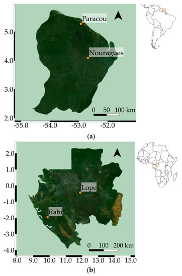
Figure 1.
French Guiana (a) and Gabon (b) study sites (ESRI Satellite®).
As for Gabon, the first site is located in Lope National Park, one of the largest national parks in central Gabon (Figure 1b). The site is mostly characterized by compact and humid tropical forests with complex structure and high AGB values (superior to 400 Mg/ha) [25]. The topography of Lope National Park is diverse, varying between large flat plains and steep slopes. The ground elevation ranges between 200 and 600 m asl, and tree heights reach up to 60 m with an average value of about 40 m [25,26]. The second site is the Rabi Forest Monitoring Plot, located near the Rabi Oil Concession (Figure 1b). It is characterized by dense humid rainforests and a fairly flat topography (ground elevation ranging from 31 to 82 m asl). Top-of-canopy height reaches up to 50 m, with the average value around 35 m [26,27].
The areas of interest considered in this study have been widely used in other similar works [22,25,26,27] due to the fact that they are specifically protected for research activities and conservation purposes. It can be fairly said that no major impacts or changes caused by anthropogenic activities have occurred recently. Nouragues is an ecological research station operated by the French National Center for Scientific Research (CNRS), and Paracou has been used as a research station to study Amazonian forest ecosystems since 1982. Similarly, Lope is a protected National Park in Gabon and was added to the World Heritage List by UNESCO in 2007. Finally, Rabi Forest Monitoring Plot is part of the Gabon Biodiversity Program and provides data for studies of carbon dynamics and biodiversity.
The four study sites correspond to zones with similar structural properties in terms of average heights and AGB levels. Nevertheless, they also differ in climate, biodiversity, elevation and slope, among other things. For the purpose of this study, all the data related to each site were merged together to create a single database describing a tropical context. The total area of natural equatorial forest covered by the merged study sites amounts to 100 km2.
2.2. Data
2.2.1. GEDI Data
GEDI-processed data are produced by NASA’s Land Processes Distributed Active Archive Center (LP DAAC). Datasets used in this study consist of both the L1B (Level 1) and L2A (Level 2) processing level. The L1B data product includes geolocated corrected and smoothed waveforms, as well as their ancillary parameters. The L2A data product provides waveform interpretation through footprint-level elevation and height metrics, including ground elevation, canopy top height and relative height (RH) metrics. The L2A product is derived from the received waveforms contained in the L1B product using six possible signal processing configurations (referred to as algorithm setting groups). Algorithm setting groups define thresholds and smoothing settings used to interpret the received waveform and therefore affect the height metrics produced in the L2A data product. Six distinct set of values are used as shown in Table 1. Therefore, for each GEDI footprint, six different canopy height values are available depending on the algorithm setting group used to process the received waveform.

Table 1.
GEDI L2A product algorithm setting groups. σ is the standard deviation of the background noise level of the received waveform.
Over the four sites considered in this study, GEDI shots (i.e., a received waveform associated with a footprint on the ground) acquired in the period between April 2019 and August 2021 were collected. Since atmospheric conditions can negatively affect the measurements carried out by the GEDI sensor, several preliminary filters were applied in order to only keep usable and relevant shots for the analysis:
- Shots with no mode detected (num_detectedmodes = 0) were removed. A signal with no mode is pure noise and does not contain any information related to the vertical structure of the forest.
- Shots with a null SNR (SNR = 0) were removed. These shots are also pure noise. Information about the computation of SNR can be found in [28].
- Shots with an erroneous detection of the ground were removed. The quality assessment of the ground detection provided by GEDI data is performed using the corresponding Shuttle Radar Topography Mission (SRTM) digital elevation model (DEM). If the absolute difference between the elevation of the lowest mode (elev_lowestmode) and the SRTM DEM (digital_elevation_model_srtm) is bigger than 100 m, then the shot is discarded.
- Shots with an incomplete waveform were removed. An incomplete waveform does not have a sufficient number of bins to be interpretable. If the end location of the usable portion of the waveform (search_end) is equal to the total number of bins in the waveform (rx_sample_count), then the waveform is considered incomplete.
- Shots with a distance between the canopy top and the ground return (rh_100) lower than 3 m were removed. These shots most likely correspond to bare soil or low vegetation and therefore are of no interest in this study.
After the filtering steps, and considering the availability of ground truth data, a total of 3864 GEDI footprints were retained for the combined analysis of the four sites described in Section 2.1 (Figure 2).
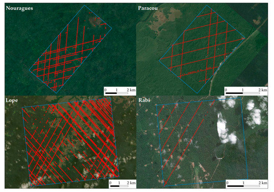
Figure 2.
ALS acquisition areas (blue) and filtered GEDI footprints (red) over the four study sites (ESRI Satellite®).
2.2.2. Reference Data
In order to assess the accuracy of GEDI data to estimate forest heights, CHMs derived from ALS data were used as ground truth. Regarding the French Guiana study sites, two airborne LiDAR surveys were conducted by private contractors in 2008 and 2012. Considering Gabon sites, the CHMs were produced in the framework of the AfriSAR mission, a collaboration between NASA and ESA conducted in the year 2016.
The four study sites are characterized by relatively high AGB levels (see Section 2.1) and tree heights. More than 80% of the GEDI footprints retained in this study correspond to heights superior to 30 m, and almost 90% of the footprints present a reference height superior to 20 m. In the context of old-growth tropical rainforest landscapes, some studies have assessed the canopy dynamics over large time spans. Based on two LiDAR datasets from 1998 and 2005 acquired over La Selva (a tropical biome in Costa Rica, Central America), Dubayah et al. [29] reported a net loss in height of −0.33 m for old-growth forests and a net gain of 2.08 m for secondary forests over a 7-year period. Kellner et al. [30] also analyzed two LiDAR datasets obtained nearly in the same periods over La Selva (1997 and 2006, corresponding to a 8.5-year time span) and found a mean change of height of −0.32 m for old-growth landscapes. Although the height does not change on average, it can vary locally by increasing or decreasing. In the same study, Dubayah et al. [29] reported local variations of about +/− 3 m over a 7-year period. Nevertheless, the dispersion that will be observed between GEDI-derived heights and airborne LiDAR CHMs is linked to many factors such as GEDI geolocation accuracy, measurement uncertainties and local variations of heights in the time span between acquisitions.
Specifically in French Guiana, according to calculation methods based on atmospheric inversion, AGB increases of about 0.5% each year [13]. If the totality of this increase were linked to tree heights, it would imply a growth of 5% in heights in a 10-year time span, resulting in a 1.5 m augmentation in this time interval (5% of 30 m, if we consider 30 m as the reference height of mature forest environments in French Guiana). In reality, in old-growth forest environments, the increase in AGB levels is mostly due to the increase in basal area rather than tree height [31,32]. Additionally, secondary forests account for a part of this AGB increase. Therefore, the actual height increase in old-growth forest ecosystems such as the ones in Paracou and Nouragues should be significantly smaller than 1.5 m in the period between the airborne LiDAR surveys and the GEDI acquisitions (approximately 10 years).
The CHM for each study site was obtained by subtracting the digital terrain model (DTM) from the digital surface model (DSM), which are both derived from the ALS data. Reference CHMs consist of raster datasets with a grid size (spatial resolution) of 1 m. Details on canopy model construction can be found in [33,34]. Considering all four sites, the total forest area covered by reference data for tree heights equals 100 km2.
2.3. Methodology
The scope of the work presented in this study can be divided into two main tasks. Firstly, assuming that a GEDI height metric can be directly used to estimate canopy heights, we assessed the influence of GEDI acquisition and processing parameters on the estimation accuracy by comparing GEDI-derived heights with the reference CHM. We focused on the impact of the algorithm setting group (six possible configurations) and of the laser beam type (two beam types). The influence of other signal parameters such as beam sensitivity and SNR was also studied. Secondly, in light of the results obtained in the first task, we developed and improved the canopy height estimation task by implementing regression models based on either GEDI metrics (L2A product) or GEDI waveforms (L1B product). Several linear and non-linear regression models were evaluated in order to estimate canopy heights from GEDI data. Finally, the generalization of these models was also tested: they were built considering various training strategies depending on the data from the available study sites.
2.3.1. Data Processing
The GEDI L2A product provides information on each acquired footprint and allows for describing them by a unique ID and a set of values corresponding to signal metrics and acquisition parameters. Regarding reference data, four raster datasets representing canopy heights for each study site are available for the analysis.
Using the geolocation of the received waveforms, with an expected geolocation accuracy of about 10 m, GEDI footprints are overlaid with the CHM rasters. For every footprint that is deemed usable in the GEDI L2A product (see Section 2.2.1), the maximum value of the CHM raster cells contained within the extent of the footprint (a 25 m circle) was extracted. This value is considered the reference canopy height for a given footprint and is referred to as ALS-CHM in this study. The maximum value of the CHM raster cells was chosen because it is theoretically closer to the top-of-canopy signal obtained from GEDI waveforms. Adam et al. [35] justified using the maximum value by the fact that return waveforms start at the highest point of vegetation within the footprints. In a similar study where they compared ALS reference heights with spaceborne LiDAR-derived height estimates, Hilbert and Schmullius [36] obtained better correlations when using the maximum rather than the mean value. Therefore, in this study, we assume that the maximum CHM value within the extent of the footprint is relevant to compare with GEDI canopy heights (referred to as GEDI-CHM).
2.3.2. Direct Estimation
In order to assess the potential of GEDI for the estimation of canopy heights, we firstly decided to use one metric from the L2A product as GEDI-CHM. Among all the available values, we identified two relevant metrics to choose between: rh_100_an or rh_95_an, with n identifying the algorithm setting group (1 to 6). Relative height metrics give the height at which a certain percentile returned energy is reached relative to the ground. For example, rh_100_a5 informs on the height at which 100% of the waveform energy is reached, in the signal processing configuration of algorithm setting group number 5. Relative heights of high percentiles are thus good indicators of canopy heights. Regarding the two specific relative heights that were identified, they are strongly correlated as shown in Figure 3.
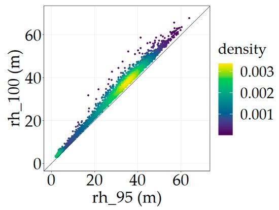
Figure 3.
Correlation between GEDI relative heights of percentiles 95 and 100 (R2 = 0.99).
In the case of direct estimation of canopy heights, we used the rh_95_an metric as the value for GEDI-CHM, in accordance with assumptions taken in previous works in the literature [37,38,39,40]. The relative height at which 95% of the signal energy is contained is directly interpreted as the estimated canopy height for a given footprint (GEDI-CHM). Since the study sites are characterized by relatively low slopes, topographic factors were not used to account for slope effects. Regarding the impact of topography, Fayad et al. [41] observed that the estimation of canopy heights from uncorrected GEDI waveforms degraded by a maximum of 1 m for slopes between 11° and 24°. For values below 11°, Fayad et al. [41] noted that the effect of slopes was minimal, with comparable accuracies over the 0–6° and 6–11° ranges. More than 90% of the footprints considered in this study present a mean slope value inferior to 24°, and 60% of the data correspond to slope values in the 0–11° range. In this perspective, given their limited impact on canopy height estimates in the context of low-sloped terrains, topography factors were not taken into account when extracting height metrics from GEDI data.
The accuracy of GEDI estimates is achieved by comparing this value to the reference canopy height derived from the reference raster datasets (ALS-CHM). For the statistical analysis and quantifying the performances of this approach, footprints with ALS-CHM values over 70 m were removed since they most likely do not represent realistic vegetation heights. In order to quantify the accuracy, the root mean square error (RMSE) and the differences between GEDI-CHM and ALS-CHM (GEDI-CHM–ALS-CHM, henceforth referred to as CHM-Differences) are calculated. To account for the fact that CHM-Differences are not normally distributed, two robust metrics used in similar studies [35,42] were chosen for their statistical description: the median and the median absolute deviation (MAD).
For each algorithm setting group (six possible configurations), GEDI-CHM was estimated using the corresponding GEDI height metric (rh_95_an, with n being the algorithm setting group) and compared to ALS-CHM, allowing for the evaluation of performances for each configuration. Additionally, the L2A product provides a variable named selected_algorithm, which corresponds to the algorithm setting group with the lowest non-noise ground return for a given footprint. With this information, GEDI-CHM was computed using the rh_95 value associated with the GEDI-selected algorithm setting group, thus creating a new mixed configuration that was also assessed in our investigations.
Regarding the beam type, a GEDI return waveform is acquired from either a coverage or a power beam, depending on the on-board laser that was used to generate the emitted pulse. Coverage and power beams differ in terms of laser power, with the former being produced at an energy level of 5 mJ while the latter are twice as strong at 10 mJ. The intensity of the beam affects its ability to penetrate the vegetation canopy to detect the ground and thus has a major influence on GEDI canopy height metrics. To quantify this influence, the GEDI L2A dataset was split according to beam type, and GEDI-CHM was compared to the corresponding ALS-CHM, allowing for highlighting the differences in performances between each beam type for the estimation of canopy heights.
GEDI’s canopy height estimation accuracy is directly linked to the laser ability to penetrate through the vegetation and to detect the ground. Identifying the ground peak in the waveform signal is of paramount importance to estimate canopy heights from a relative height metric such as rh_95. An incorrect ground peak detection in a waveform signal can be explained either by the fact that the laser could never reach the ground or because the ground mode is too hard to isolate from the noise that characterizes every numeric signal. In this prospective, sensitivity and SNR are also two fundamental signal parameters that allow for understanding and characterizing these scenarios. Firstly, beam sensitivity is defined as the maximum canopy cover that can be fully penetrated all the way to the ground by the laser. A high sensitivity allows for the signal to penetrate denser canopies and thus to reach the ground. Secondly, SNR is a commonly used measure that compares the level of a desired signal to the level of background noise [28]. A high SNR implies a better extraction of the useful parts of the signal to perform the metrics computation. The influence of these parameters on GEDI-CHM was assessed to understand how they affect canopy heights estimates.
2.3.3. Regression Models
GEDI relative height metrics are good indicators of forest heights. The simplest method to estimate the canopy height from a GEDI waveform is to use a single metric derived from the waveform and to consider that it directly represents the canopy height. In the case of this study, we first used the relative height at which 95% of the waveform energy is reached (rh_95_an). However, over densely forested areas with high AGB levels, it is harder for the laser signal to penetrate the vegetation and to detect the ground, making the identification of the ground peak in the received waveform difficult and the estimation of forest height inaccurate [20]. In this prospective, statistical approaches have been developed and used in several studies to predict canopy heights from GEDI data [4,23,43]. These methods proposed regression models based on waveform metrics. Rather than using a single metric, GEDI-CHM is therefore the result of a model built on several pre-selected GEDI L2A waveform metrics (see Table 2). In addition, in the same spirit, deep learning approaches allowed for estimating canopy heights directly from the geolocated waveforms of the GEDI L1B data product [21,44]. In that case, GEDI-CHM is the result of a model trained and validated on the GEDI L1B received waveforms.

Table 2.
GEDI L2A variables to be used as predictors in the canopy height regression models.
In this study, three types of models were implemented and evaluated using ALS-CHM reference data: a stepwise multilinear regression (SRH), a random forest (RF) regressor and a convolutional neural network (CNN) encoder. To assess how the models perform and how they can be generalized to an independent dataset, a ten-fold cross validation was used, and the RMSE as well as the CHM-Differences were computed. This process was either applied on the whole available dataset (i.e., the four sites merged into a single database) or on sub-samples corresponding to the data of a given country (Nouragues and Paracou altogether on one hand, Lope and Rabi on the other). The purpose is to highlight if the availability of reference data is of interest to create general estimators that can be applied at a larger scale to other areas with similar heights and AGB levels. In addition, for the sake of completeness and to understand how these approaches could be generalized to other study sites, the models were also built on the data available for each country and were tested directly on the other one.
Firstly, a SRH was implemented to estimate canopy heights by automatically selecting a set of predictive explanatory variables among all possible predictors presented in Table 2. The choice of adding or removing a variable from the SRH linear model is based on the variation of the mean squared error (MSE). In this approach, the target variable is estimated through a linear relationship between the most relevant predictors. Canopy heights were also estimated through non-linear non-parametric regressions using a random forest (RF) regressor. The RF method is a machine learning algorithm that leverages ensemble of trees via a bagging strategy to estimate the target variable. Compared to SRH, RF has the advantage of being able to model non-linear relationships between the predictors. In this analysis, we used the explanatory variables described in Table 2, and the number of trees was set to 500. The importance of the predictors used as input for the regression can be quantified in order to understand the most contributing factors in the estimation of the target variable. Finally, CNN encoders such as those described in [21] were developed to predict canopy heights from GEDI waveforms. CNN architectures implement the convolutional operation and allow for dealing with the temporal autocorrelation that characterizes numeric signals such as the L1B waveforms. Compared to the previous models, these approaches rely solely and directly on the received GEDI waveform signals. In order to extract an extensive amount of signal features and to capture localized information in the input waveforms, we set a small kernel size equal to 3 for the convolution operations.
3. Results
3.1. Using rh_95
3.1.1. GEDI-CHM Accuracy
The results presented in Figure 4 are scatter plots of GEDI-CHM and ALS-CHM values for each algorithm setting group. They exhibit a quite weak linear correlation ranging from 0 to 0.30 (R2 coefficient). The most notable feature that characterizes the distributions is a high number of footprints where GEDI significantly underestimates canopy height. GEDI’s ability to correctly estimate tree heights is linked to its ability to detect the ground below and is therefore directly correlated to the laser penetration through the vegetation.
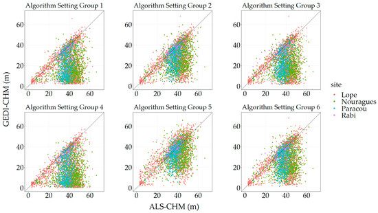
Figure 4.
GEDI-CHM estimated from rh_95 as a function of ALS-CHM for each algorithm setting group.
The accuracy metrics displayed in Table 3 confirm the results implied by the scatter plots. Algorithm setting group number 5 performs the best to estimate CHM with a median CHM-Differences of −1.5 m and a RMSE of 11.6 m. Other algorithms show a relatively low accuracy, with setting group numbers 1, 3 and 4 being less accurate. Algorithm setting group numbers 2 and 6 exhibit similar performances since they have similar signal processing settings. Finally, the GEDI-selected algorithm provided in the L2A product outperforms all the algorithms except for the number 5.

Table 3.
Accuracy of GEDI-CHM estimates using rh_95 height metric derived with different algorithm setting groups.
3.1.2. Influence of GEDI Beam Type
Focusing on the influence of beam type, the same trends can be observed, and the same conclusions can be drawn regardless of the algorithm setting group that was used. Therefore, in order to assess and understand the influence of beam type on GEDI’s ability to estimate canopy heights, we focus on algorithm setting group number 5 since it performs better than all its competitors.
Boxplots in Figure 5a describe the distributions of CHM-Differences depending on beam type. A clear shift in accuracy can be observed with respect to beam type, and it is confirmed by the values reported in Table 4. The median of CHM-Differences from coverage beams is greater in absolute value than the median of CHM-Differences from power beams, the former being at −9.1 m while the latter is at 1.2 m. In addition, CHM-Differences are in general higher in absolute value for footprints acquired through coverage beams (Figure 5a). In a notable way, GEDI coverage beams tend to underestimate CHM, whereas no such observation can be made for power beams.
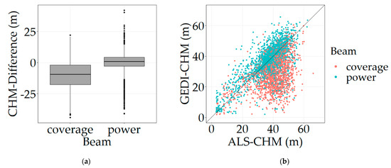
Figure 5.
Boxplots of the CHM-Differences (a) and GEDI-CHM as a function of ALS-CHM (b) depending on beam type (algorithm setting group number 5).

Table 4.
Accuracy of GEDI-CHM estimates using rh_95 height metric depending on beam type (algorithm setting group number 5).
Figure 5b provides a visual representation to appreciate the difference in CHM estimation accuracy between coverage and power beams. The linear correlation is stronger for footprints acquired through power beams, with an R2 value of 0.70 instead of 0.25 for coverage beams.
3.1.3. Influence of Sensitivity and SNR
Figure 6 exhibits the relation between CHM-Differences and sensitivity on one hand, and between CHM-Differences and SNR on the other. As highlighted by the trendlines, GEDI footprints with a higher sensitivity and SNR show a better accuracy for the estimation of canopy heights. A low sensitivity implies a bad ground height estimation because the signal is not able to penetrate dense vegetation all the way through, resulting in an overestimation of ground heights and therefore an underestimation of canopy heights. Similarly, a low SNR makes the ground mode harder to identify and extract, either because it is too weak or too noisy, and this results in an underestimation of canopy heights.
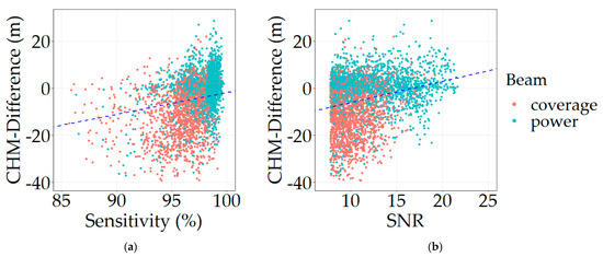
Figure 6.
CHM-Differences as a function of sensitivity (a) and SNR (b) for algorithm setting group number 5. The blue dashed lines represent the trendlines (linear).
Additionally, when considering beam type in this analysis, coverage beams tend to be associated with lower sensitivities and SNR (Figure 6), whereas power beams do not show a tendency to underestimate canopy heights (Figure 5 and Figure 6). The laser power has a direct influence on signal parameters such as sensitivity and SNR, which in turn are decisive for accurate canopy height estimates.
3.2. Using Regression Models
3.2.1. GEDI-CHM Accuracy with Models Based on Waveform Metrics
In this section, we evaluate the performances of SRH and RF regressors built on the metrics defined in Table 2. Figure 7 shows the RMSE and MAD of GEDI-CHM for each estimator based on the GEDI L2A product. The results highlight the fact that using regression models built on waveform metrics allows for significantly improving the results of the estimation task compared to the direct method. Algorithm setting group number 5 exhibits the best performances for all three estimators, and RF appears to be the best approach regardless of which algorithm setting group is used. For example, when considering algorithm setting group number 5, the RMSE improved from 11.6 m with a direct estimation of 8.0 and 6.7 m with the SRH and RF models, respectively. Moreover, these models show that they are less dependent on the algorithm used to compute the waveform metrics than the direct method, with RF being the most stable approach in this regard.
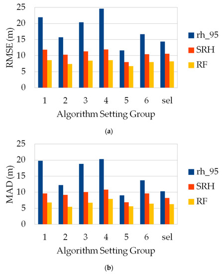
Figure 7.
RMSE (a) and MAD (b) for GEDI-CHM estimators (10-fold cross validation, whole dataset) depending on algorithm setting group: direct estimation, SRH and RF. “sel” corresponds to GEDI-selected algorithm.
When the analysis is carried out according to beam type, a clear shift in performances is observed between the two laser types. Since algorithm setting group number 5 displays the best performances in GEDI-CHM estimations, further performance analyses in this paper are presented for this specific configuration. Figure 8 shows the RMSE and MAD of GEDI-CHM estimates for the competing estimators depending on the footprints’ beam types. The main result that can be drawn is that power beams generally perform better than coverage for the estimation task regardless of the method used. Moreover, similarly to what was previously observed concerning the model stability in relation to the algorithm setting group, SRH and RF regressors exhibit relatively close performances between power and coverage beams, with RF being the most stable approach once again: the RMSE reaches values of 5.9 and 7.7 m for power and coverage beams, respectively (Figure 8a). Finally, power beams show a relative stability for GEDI-CHM estimations since the results obtained are of similar magnitude regardless of the method used, with RMSE values ranging from 5.9 to 8.1 m (Figure 8a).
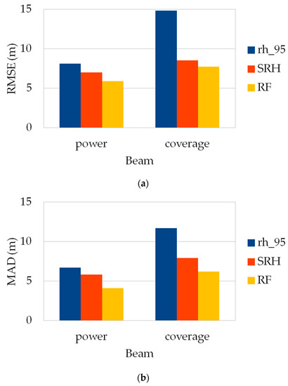
Figure 8.
RMSE (a) and MAD (b) for GEDI-CHM estimators (10-fold cross validation, whole dataset) depending on beam type (algorithm setting group number 5): direct estimation, SRH and RF.
3.2.2. Variable Importance for Models Based on Waveform Metrics
In this section, we present the variable importance analysis of SRH and RF regressors. Firstly, the SRH model automatically selects the most relevant predictors among all the available inputs and produces a linear relation, allowing for linking CHM with the most explanatory variables. Before the implementation of the SRH model, sensitivity was converted to a binary parameter. Its value is defined depending on a certain threshold: for a given GEDI footprint, if the sensitivity is superior to 98%, then the value is set to 1 (reciprocally to 0 if the sensitivity is inferior to 98%). Similarly, beam type was also converted to a Boolean value: 0 for coverage beam and 1 for power. These binary parameters are used as input variables in the SRH model implementation. When considering all the available data (i.e., 3864 GEDI footprints), the relation built by the SRH model is the following:
GEDI-CHM (m) =
22.5 − 0.6 × wext − 0.3 × lead + 1.3 × rh_95 + 1.2 × sensitivity − 6.9 × beamtype
22.5 − 0.6 × wext − 0.3 × lead + 1.3 × rh_95 + 1.2 × sensitivity − 6.9 × beamtype
Waveform extent (m), leading edge extent (m), rh_95 (m), sensitivity and beam type are automatically selected as the most contributing variables in CHM estimation.
Secondly, regarding RF, the analysis of the importance informs about which variables have the most predictive power (Figure 9). Beam type appears as the most important variable for CHM estimation. In order to be able to compare all regressors on a fair basis, the categorical beam sensitivity values are also used as RF input variables, and sensitivity emerges as a key predictor. Waveform extent and leading edge extent still bring a significant contribution in a similar way to what has been observed for SRH. Concerning relative heights, rh_10 and rh_100 are the most contributing input variables when estimating CHM through a RF model.
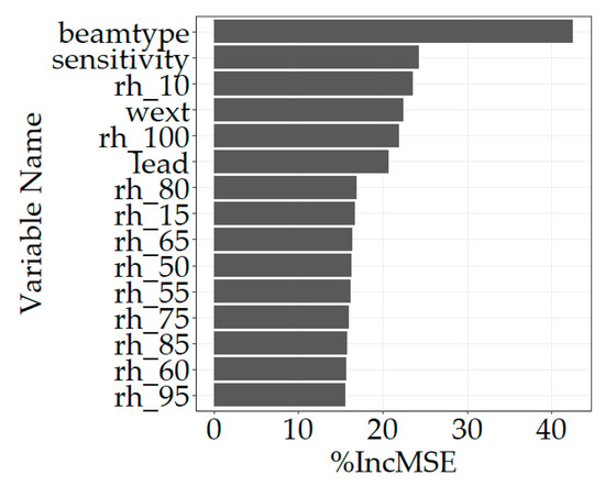
Figure 9.
Importance of RF variables (fifteen most important) using mean decrease accuracy (%IncMSE).
3.2.3. Model Transferability
To study the viability of model transferability across study sites, several training options were considered given the variety of data in the dataset used in this study. In this section, we focus on the use of RMSE to evaluate performances. Regarding the strategies to train and validate models, a total of five approaches was adopted as reported in Table 5. These approaches rely on different partitions of the whole dataset for the training and validation of models.

Table 5.
RMSE for GEDI-CHM SRH and RF estimators depending on training/validation strategies (algorithm setting group number 5).
Figure 10 gives a graphical representation of the results reported in Table 5. When considering strategies relying on a 10-fold cross validation (“Full”, “Guiana” and “Gabon”), RF shows significant stability in terms of performances, with identical values of RMSE for each configuration (6.7, 6.9 and 6.5 m, respectively). SRH is more sensitive to the dataset used to build the model but also remains quite stable, with RMSE values ranging from 7.0 to 8.2 m. Regarding strategies that are based on country training (training on one country, validation on the other), they exhibit degraded performances in terms of RMSE, with “Guiana > Gabon” being by far the least interesting approach for both SRH and RF estimators.
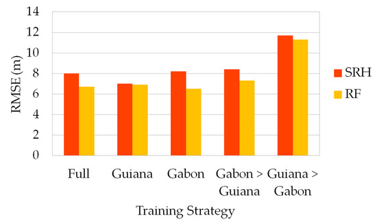
Figure 10.
RMSE for GEDI-CHM SRH and RF estimators depending on training/validation strategies (algorithm setting group number 5).
3.2.4. GEDI-CHM Accuracy with Models Based on Waveforms
CNN encoders are directly built on the waveforms available in the GEDI L1B product and therefore are not dependent on algorithm setting group since the signal is directly processed as is, and no metrics extracted from it are used. In order to be able to compare the results of this method with its competitors, we considered the best performing algorithm setting group for the previous approaches, which is setting group number 5. Similarly to what was performed before, the CNN encoders were trained and validated following different strategies. Figure 11 shows the RMSE and MAD depending on beam type for all the methods considered in this study, trained with the “Full” strategy.
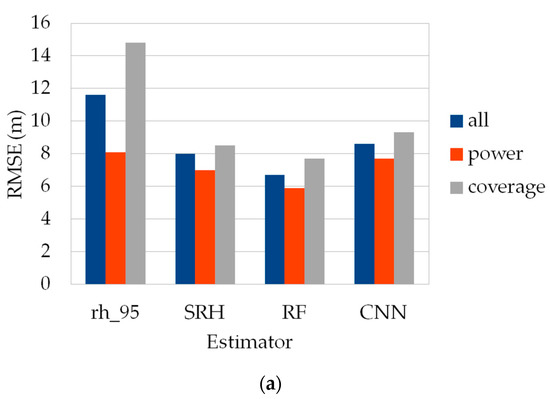
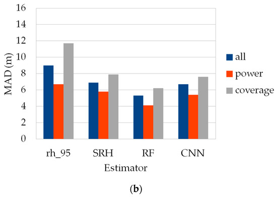
Figure 11.
RMSE (a) and MAD (b) for all GEDI-CHM estimators depending on beam type: all beams, power only and coverage only.
Regarding beam type, CNNs behave the same way as their competitors, with power beams also giving the best results in terms of RMSE. However, RF remains the best performing method to estimate CHM in all training scenarios, while CNNs are the second best. For example, when considering the common scenario of a “Full” training strategy and all beam types used, CNNs reach a RMSE value of 8.6 m compared to the best value of 6.7 m for RF.
4. Discussion
The different approaches tested in this paper to estimate canopy heights from GEDI data showed that prediction models based on waveform metrics allowed for obtaining good accuracies of heights estimates, with a best RMSE and MAD value of 5.9 and 4.1 m, respectively.
The simplest way to estimate canopy heights from GEDI data is to use a specific L2A level metric as a direct proxy of CHM. We chose to use rh_95 for this purpose, corresponding to the 95th percentile of energy return height relative to the ground. Upper relative height metrics (i.e., rh_90, rh_95 and rh_100) are related to the top of forest canopies. Potapov et al. [37] observed in their study that, in a tropical biome, rh_95 showed the highest correlation with ALS-derived reference heights, while rh_90 underestimated canopy height, and rh_100 overestimated it compared to rh_95. Neuenschwander et al. [39] made a similar observation, although in a different context of sparse boreal forests in Alaska (USA).
GEDI metrics values are based on the L2A processing algorithm, which uses six different sets of parameters to perform the waveform processing. The analysis of the GEDI-CHM accuracy with rh_95 derived from all available algorithm setting groups showed that algorithm setting group number 5 delivers a significantly better accuracy than other groups. In the tropical context of French Guiana and Gabon, forests present high AGB levels and dense canopies. The ability of GEDI to estimate canopy heights is directly dependent on its ability to detect the ground. Due to the density of the vegetation in tropical areas, the ground peak in GEDI waveforms is usually weaker in terms of intensity and is therefore harder to extract and separate from the background noise. Algorithm setting group number 5 is characterized by a lower waveform signal end threshold compared to the other setting groups. A low threshold allows for better discrimination of weak ground returns from the noise in the signal, while higher thresholds will lead in general to an error of detection. On the contrary, in less dense forest ecosystems, a low threshold can result in the interpretation of noise below the actual ground as the ground peak, leading to an overestimation of canopy heights [35,43]. GEDI waveforms acquired over tropical forests usually present weaker intensity ground peaks compared to other less dense forest environments, allowing for the conclusion that a lower signal end threshold such as the one characterizing algorithm setting group number 5 seems more adapted in this specific context. The results obtained with algorithm setting groups number 1, 3 and 4 are in the same direction as this observation: they are characterized by the highest signal end threshold among all possible configurations and are proven to be the least accurate when estimating canopy heights from rh_95.
The assessment of GEDI canopy height estimates is based on reference heights obtained from ground truth data. Each GEDI footprint is described by a unique reference height that is compared to the canopy height derived from the selected GEDI metric. In this prospective, the maximum CHM value in the footprint’s extent appears to be better correlated to GEDI height metrics since the toploc of the waveform (i.e., the location of the highest detected return in the waveform) is associated with the first laser-environment interaction that occurs with the highest object within the footprint [35,36]. For the sake of completeness and in order to consider another proxy for ALS-CHM, the accuracy assessment of GEDI canopy height estimates was also performed using the mean CHM value within the footprint as the reference height value (Table 6).

Table 6.
Accuracy of GEDI-CHM estimates using the mean height value for ALS-CHM.
When using the mean height value as ALS-CHM, the most notable observation that can be drawn is that the tendency to underestimate canopy heights is greatly lessened. For example, the least performing algorithm setting groups (groups number 1, 3 and 4, as stated previously) still present a negative median CHM-Differences but significantly lower in terms of absolute value. On the contrary, the other better performing algorithm setting groups tend to slightly overestimate canopy heights, especially algorithm setting group number 5, which is characterized by a lower waveform signal end threshold. The choice of either the mean or the maximum value to extract the ground truth greatly impacts the reference heights that are used for the accuracy assessment of GEDI canopy height estimates. Over the 3864 footprints that were retained in this study, the mean difference between mean ALS-CHM and maximum ALS-CHM amounts to −10.1 m (−9.4 m for the median), with a standard deviation of 5.3 m. The observed attenuation of the height underestimation for all algorithm setting groups could then be linked to the fact that reference heights given by mean ALS-CHM are significantly lower than the actual heights as seen by GEDI waveforms. Therefore, in accordance with assumptions taken in related works [35,36], the maximum ALS-CHM is deemed more relevant to compare with GEDI height metrics.
The signal capability to penetrate through the forest and reach the ground is closely linked to the laser’s physical properties. GEDI’s power beams are twice as powerful as coverage ones in terms of laser energy, which directly affects the penetration of dense canopies. Fayad et al. [20] observed that coverage lasers exhibited a significantly lower level of performance for tree height estimation in comparison to other full power configurations such as GEDI and NASA’s Land Vegetation and Ice Sensor (LVIS). The analysis performed in our study delivered similar results, with power beams showing a clear advantage for CHM estimation compared to coverage beams. The main observation that was drawn is a tendency for the latter to underestimate tree heights, whereas the former exhibited a quite strong linear correlation with reference canopy heights. Pulses emitted with coverage lasers generally have more difficulty reaching the ground because of the density of the vegetation, and consequently, the mode extracted as the ground peak in the waveforms is located at a higher height than the actual ground elevation, thus resulting in an overestimation of the ground height and therefore an underestimation of canopy heights. On the contrary, power beams seem to be able to penetrate the vegetation all the way vertically and produce received waveforms with a recognizable lowest mode corresponding to the actual ground. When using GEDI data for canopy height retrieval, Liu et al. [45] noted that beam strength had a strong impact on the obtained results and recommended the use of only strong/power beam data for better CHM estimates. We reached the same conclusion in light of our study, with an improvement of about 80% and 75% in terms of RMSE and MAD, respectively, when comparing coverage and power beams for CHM estimation through rh_95.
The waveform interpretation and metrics computation are also very dependent on the signal quality and shape. The physical properties of the received signal that is processed by GEDI have a major influence on the obtained L2A level metrics, and thus on the CHM estimation through rh_95. The results obtained in this study highlight the fact that beam sensitivity is a parameter of major importance for CHM estimation. The higher the sensitivity, the better the signal that can penetrate the vegetation and detect the ground. Using rh_95 as a direct proxy of CHM requires a correct detection of both the ground peak and the canopy top in the waveform in order to be able to interpret this value as the actual canopy height. Over densely vegetated areas such as the ones considered in this study, the reflection off the ground that is recorded by GEDI sensors can be very weak, if not totally absent. Footprints characterized by a high sensitivity generally allow for a better detection of the ground return since these shots can penetrate denser canopy covers. In this prospective, Fayad et al. [20] concluded that footprints with a sensitivity higher than 98% showed a deeper penetration of the vegetation, as the rh_100 value increased by 5 m on average for both power and coverage beams. Although they considered another height metric than the one we used, the strong correlation between rh_95 and rh_100 allows for drawing the same conclusion regardless of the metric used. Our results also highlight a connection between beam sensitivity and beam type (Figure 6). When exploring this connection in more detail, it appears that power beams are characterized by increased values of sensitivity (Figure 12), which is consistent with the fact that stronger lasers are able to penetrate through denser canopy covers. In addition, the threshold of 98% that was used by Fayad et al. [20] to remove shots with insufficient penetration roughly discriminates between power and coverage beams in our case.
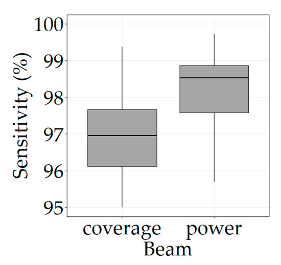
Figure 12.
Relation between beam type and beam sensitivity (algorithm setting group number 5). Outliers removed for clarity.
Regarding SNR, the higher it is, the easier it is to correctly interpret the waveform and extract the ground peak from the background noise. When considering the influence of SNR according to beam type, power and coverage beams behave in different ways (Figure 6): while the former show a certain stability for the estimation of CHM, with no significant differences between low and high values of SNR, the latter exhibit a tendency to underestimate canopy heights in low ranges of SNR. The stability of power beams advocates for the fact that, even in the context of noisy waveforms, beam sensitivity is the most impactful parameter for CHM estimation, as it is directly linked to ground detection. A weak ground mode in a given waveform is not necessarily a synonym of bad canopy height estimate if its location really corresponds to the actual ground elevation. In addition, similarly to the observation made before for sensitivity, power beams are characterized by increased values of SNR, which is also consistent with the fact that stronger lasers tend to be less sensitive to background noise.
Overall, the accuracies obtained when using rh_95 as a direct proxy of CHM remain insufficient to consider this method as satisfying. The use of statistical approaches based on GEDI L2A metrics induces significant improvements on CHM estimates [4,23,43]. Rather than considering a single metric, multiple predictors are used as input to build and train empirical models. The approaches evaluated in this study allow for taking advantage of the richness of the information contained in the waveforms and for leveraging the interplay between all the predictors to estimate the target variable. The predictors that were selected to perform this task correspond to height metrics describing the canopy tops, the ground elevation and the vertical structure of the forest. These variables are correlated to tree heights and are often used in canopy height estimation [4,23,43]. Signal parameters such as beam type and beam sensitivity were also added as input variables since they proved to strongly impact the direct CHM estimation through rh_95. The implementation of a SRH model shows that waveform metrics can be used to obtain significantly better accuracies of CHM. When using all the available data to build the model, we reach notable improvements of 45% and 30% in RMSE and MAD, respectively, compared to the use of rh_95 as a direct proxy of CHM. The model automatically selects the most relevant predictors among all the available inputs and produces a linear relation allowing for the identification of the most explanatory variables. Waveform extent, leading edge extent, rh_95, sensitivity and beam type emerge as the most important GEDI variables for the estimation of CHM. Waveform extent is one of the most used waveform metrics to estimate CHM through linear models. Lefsky et al. [4] firstly developed a statistical model that was based only on the waveform extent to estimate the maximum canopy height. Payn et al. [46] then incorporated the waveform leading edge extent and obtained slightly improved results on canopy height estimation. The leading edge extent characterizes the detection of canopy tops and, in our case, is selected as a major factor of CHM variability. As stated many times before, rh_95 is one of the most correlated GEDI metrics with ALS reference heights, and it is therefore natural to prove as a significant contributor to CHM estimates. Finally, consistent with the analysis performed in this paper, sensitivity and beam type are two fundamental signal parameters that appear in Equation (1) because they are linked to GEDI’s ability to detect the ground and, consequently, to derive relevant height metrics from the received waveforms.
RF is commonly used for the prediction of forest attributes when reference ground truth data are available. In the context of this study, RF shows a strong capability to leverage the available inputs to produce good CHM estimates. This method proves to be both the most accurate and the most stable regarding all the parameters of influence that were considered. The accuracies of CHM estimates remain in the same order of magnitude no matter which algorithm setting group is used (RMSE ranging from 6.7 to 8.6 m). Moreover, when considering the impact of beam type, RF is also capable of exploiting the information given by waveform metrics regardless of the configuration of the acquisition (RMSE of 5.9 and 7.7 m for power and coverage beams, respectively). The analysis of the importance informs about which variables have the most predictive power. Figure 9 shows that the variables that were previously selected by the SRH model still appear as impactful predictors for the CHM estimation task using RF. In particular, as highlighted and discussed before, beam type and sensitivity are key inputs for the models, as they are directly linked to laser penetration and ground detection. The importance of rh_10 can be explained by the fact low percentiles of relative heights (rh_10 and rh_15 especially) provide information about the deep layers of the forest and thus are related to the laser penetration. Reciprocally, rh_95 still appears as an explanatory predictor for canopy heights, as well as rh_100.
The CNN encoders implemented in this study did not allow for obtaining significant gains in performances, as they produced CHM estimates with accuracies similar to the ones of SRH regressors. Deep learning approaches and especially neural networks rely on the availability of big amounts of data for model training. The limited sample size of the dataset used in this analysis (less than 4000 usable GEDI footprints) may not be adequate to exploit the full capacity of these methods. Nevertheless, CNNs have the huge advantage of directly taking the L1B product as input (i.e., the waveforms), thus avoiding the extraction of descriptive metrics from the signals. As highlighted many times before, some metrics are harder to extract depending on the signal parameters, especially the ones linked to the ground detection, and therefore, it can be interesting to skip this step that may alter the waveform information and give uncertain results.
Finally, the testing of several training options advocates for the viability of model transferability across study sites that are characterized by comparable tree heights and AGB levels. Each training configuration gave similar results in terms of RMSE for both SRH and RF, except for the “Guiana > Gabon” strategy. The French Guiana ground truth data cover a smaller range of tree heights (between 21 and 58 m) compared to the Gabon dataset (between 4 and 62 m), which poses a problem for a method such as RF that is unable to extrapolate and is limited within the range of the training sample. On the contrary, the “Gabon > Guiana” strategy performed similarly as the “Full” one given the fact that the training sample covers a wide range of tree heights. All things considered, a sufficient and diverse training set is always necessary for statistical approaches and empirical models built on reference data. Such models could then be transferred and applied on other study sites that share similar structural characteristics.
5. Conclusions
In this study, several approaches to estimate CHM from GEDI data were tested while assessing the impact of GEDI acquisition and processing parameters on the accuracy of canopy height estimates. The tested methods can be classified into two main categories depending on the approaches that were considered. On one hand, we used a GEDI height metric (rh_95) as a direct proxy of CHM. This method is the simplest since it relies on a single value that is directly available in the GEDI L2A product, but in return, it is also the least accurate and the most dependent on GEDI signal properties. On the other hand, statistical approaches (built on the L2A product) and deep learning frameworks (based on the L1B product) were implemented and allowed for reaching improved accuracies for CHM estimates.
All things considered, GEDI acquisition and processing parameters have a strong impact on the data derived from waveforms and, consequently, on the CHM estimates produced from these data. Firstly, the algorithm setting group defines the parameters for the smoothing of received waveforms and thus directly influences the values of the metrics extracted from the signals. Depending on the forest context, a setting group is more or less adapted for the extraction of relevant metrics. In this analysis, we observed that algorithm setting group number 5 was the most suited to correctly detect the ground peak in waveforms acquired over tropical forests. This result is quite different from comparable studies that analyzed the impact of algorithm setting groups over temperate forests, for example. Secondly, the beam type, which is linked to GEDI laser power, appears as the most impactful parameter when assessing the quality of GEDI data. Power and coverage beams differ significantly in terms of laser energy, and over tropical forests and high AGB contexts, power beams are more capable of penetrating the vegetation all the way to the ground, thus providing received waveforms accurately describing the vertical structure of the forest from the top-of-canopy to the actual ground. Thirdly, in the same spirit, beam sensitivity is also linked to the laser penetration and is a key input for canopy height estimation, especially over the dense canopies that characterize tropical biomes.
Overall, the use of rh_95 as a direct proxy of CHM exhibited relatively low accuracies. When no reference data are available (i.e., reference canopy heights), rh_95 can still be used in certain conditions to derive canopy heights. We recommend the use of only power beam data, as this configuration allowed for reaching better results compared to the use of all available footprints. In contrast, when reference data are available, the implementation of regression models induces significant improvements in CHM estimation accuracies. These approaches also show certain stability in relation to the signal acquisition and processing parameters that were assessed in this study. The key factor when building empirical models is the availability of sufficient amounts of data for model training. Depending on the data availability, the operational application and the desired accuracies, GEDI information can be used in diverse manners to estimate canopy heights.
Author Contributions
Conceptualization, K.L., N.B., G.l.M. and I.F.; Data curation, K.L., N.B., G.l.M. and I.F.; Formal analysis, K.L., N.B., G.l.M. and I.F.; Methodology, K.L., N.B., G.l.M. and I.F.; Software, K.L. and I.F.; Validation, K.L., N.B., G.l.M. and I.F.; Visualization, K.L.; Writing—original draft, K.L., N.B., G.l.M. and I.F. All authors have read and agreed to the published version of the manuscript.
Funding
This research received funding from the French Space Study Center (CNES, TOSCA 2022 project) and the National Research Institute for Agriculture, Food and the Environment (INRAE).
Data Availability Statement
GEDI data were obtained from the LP DAAC (https://e4ftl01.cr.usgs.gov/GEDI/, accessed on 29 August 2022).
Acknowledgments
The authors would like to thank the GEDI team and NASA’s LP DAAC for providing the GEDI data.
Conflicts of Interest
The authors declare no conflict of interest.
References
- Pan, Y.; Birdsey, R.A.; Fang, J.; Houghton, R.; Kauppi, P.E.; Kurz, W.A.; Phillips, O.L.; Shvidenko, A.; Lewis, S.L.; Canadell, J.G.; et al. A Large and Persistent Carbon Sink in the World’s Forests. Science 2011, 333, 988–993. [Google Scholar] [CrossRef] [PubMed]
- Asner, G.P.; Mascaro, J. Mapping Tropical Forest Carbon: Calibrating Plot Estimates to a Simple LiDAR Metric. Remote Sens. Environ. 2014, 140, 614–624. [Google Scholar] [CrossRef]
- Chave, J.; Andalo, C.; Brown, S.; Cairns, M.A.; Chambers, J.Q.; Eamus, D.; Fölster, H.; Fromard, F.; Higuchi, N.; Kira, T.; et al. Tree Allometry and Improved Estimation of Carbon Stocks and Balance in Tropical Forests. Oecologia 2005, 145, 87–99. [Google Scholar] [CrossRef] [PubMed]
- Lefsky, M.A.; Harding, D.J.; Keller, M.; Cohen, W.B.; Carabajal, C.C.; Del Bom Espirito-Santo, F.; Hunter, M.O.; de Oliveira, R. Estimates of Forest Canopy Height and Aboveground Biomass Using ICESat: Icesat Estimates of Canopy Height. Geophys. Res. Lett. 2005, 32, L22S02. [Google Scholar] [CrossRef]
- Feldpausch, T.R.; Lloyd, J.; Lewis, S.L.; Brienen, R.J.W.; Gloor, M.; Monteagudo Mendoza, A.; Lopez-Gonzalez, G.; Banin, L.; Abu Salim, K.; Affum-Baffoe, K.; et al. Tree Height Integrated into Pantropical Forest Biomass Estimates. Biogeosciences 2012, 9, 3381–3403. [Google Scholar] [CrossRef]
- Lima, A.J.N.; Suwa, R.; de Mello Ribeiro, G.H.P.; Kajimoto, T.; dos Santos, J.; da Silva, R.P.; de Souza, C.A.S.; de Barros, P.C.; Noguchi, H.; Ishizuka, M.; et al. Allometric Models for Estimating Above- and below-Ground Biomass in Amazonian Forests at São Gabriel Da Cachoeira in the Upper Rio Negro, Brazil. For. Ecol. Manag. 2012, 277, 163–172. [Google Scholar] [CrossRef]
- Boyd, D.S.; Danson, F.M. Satellite Remote Sensing of Forest Resources: Three Decades of Research Development. Prog. Phys. Geogr. Earth Environ. 2005, 29, 1–26. [Google Scholar] [CrossRef]
- Véga, C.; Renaud, J.-P.; Durrieu, S.; Bouvier, M. On the Interest of Penetration Depth, Canopy Area and Volume Metrics to Improve Lidar-Based Models of Forest Parameters. Remote Sens. Environ. 2016, 175, 32–42. [Google Scholar] [CrossRef]
- Lahssini, K.; Dayal, K.R.; Durrieu, S.; Monnet, J.-M. Joint Use of Airborne LiDAR Metrics and Topography Information to Estimate Forest Parameters via Neural Networks. In Proceedings of the 2022 IEEE 21st Mediterranean Electrotechnical Conference (MELECON), Palermo, Italy, 14–16 June 2022; pp. 442–447. [Google Scholar]
- Hancock, S.; Armston, J.; Hofton, M.; Sun, X.; Tang, H.; Duncanson, L.I.; Kellner, J.R.; Dubayah, R. The GEDI Simulator: A Large-Footprint Waveform Lidar Simulator for Calibration and Validation of Spaceborne Missions. Earth Space Sci. 2019, 6, 294–310. [Google Scholar] [CrossRef]
- Karasiak, N.; Sheeren, D.; Fauvel, M.; Willm, J.; Dejoux, J.-F.; Monteil, C. Mapping Tree Species of Forests in Southwest France Using Sentinel-2 Image Time Series. In Proceedings of the 2017 9th International Workshop on the Analysis of Multitemporal Remote Sensing Images (MultiTemp), Brugge, Belgium, 27–29 June 2017; pp. 1–4. [Google Scholar]
- Grabska, E.; Hostert, P.; Pflugmacher, D.; Ostapowicz, K. Forest Stand Species Mapping Using the Sentinel-2 Time Series. Remote Sens. 2019, 11, 1197. [Google Scholar] [CrossRef]
- Quegan, S.; Le Toan, T.; Chave, J.; Dall, J.; Exbrayat, J.-F.; Minh, D.H.T.; Lomas, M.; D’Alessandro, M.M.; Paillou, P.; Papathanassiou, K.; et al. The European Space Agency BIOMASS Mission: Measuring Forest above-Ground Biomass from Space. Remote Sens. Environ. 2019, 227, 44–60. [Google Scholar] [CrossRef]
- Lahssini, K.; Teste, F.; Dayal, K.R.; Durrieu, S.; Ienco, D.; Monnet, J.-M. Combining LiDAR Metrics and Sentinel-2 Imagery to Estimate Basal Area and Wood Volume in Complex Forest Environment via Neural Networks. IEEE J. Sel. Top. Appl. Earth Obs. Remote Sens. 2022, 15, 4337–4348. [Google Scholar] [CrossRef]
- Morin, D.; Planells, M.; Baghdadi, N.; Bouvet, A.; Fayad, I.; Le Toan, T.; Mermoz, S.; Villard, L. Improving Heterogeneous Forest Height Maps by Integrating GEDI-Based Forest Height Information in a Multi-Sensor Mapping Process. Remote Sens. 2022, 14, 2079. [Google Scholar] [CrossRef]
- Dubayah, R.; Blair, J.B.; Goetz, S.; Fatoyinbo, L.; Hansen, M.; Healey, S.; Hofton, M.; Hurtt, G.; Kellner, J.; Luthcke, S.; et al. The Global Ecosystem Dynamics Investigation: High-Resolution Laser Ranging of the Earth’s Forests and Topography. Sci. Remote Sens. 2020, 1, 100002. [Google Scholar] [CrossRef]
- Baghdadi, N.N.; El Hajj, M.; Bailly, J.-S.; Fabre, F. Viability Statistics of GLAS/ICESat Data Acquired Over Tropical Forests. IEEE J. Sel. Top. Appl. Earth Obs. Remote Sens. 2014, 7, 1658–1664. [Google Scholar] [CrossRef]
- Fayad, I.; Baghdadi, N.; Riedi, J. Quality Assessment of Acquired GEDI Waveforms: Case Study over France, Tunisia and French Guiana. Remote Sens. 2021, 13, 3144. [Google Scholar] [CrossRef]
- Herzfeld, U.C.; McDonald, B.W.; Wallin, B.F.; Neumann, T.A.; Markus, T.; Brenner, A.; Field, C. Algorithm for Detection of Ground and Canopy Cover in Micropulse Photon-Counting Lidar Altimeter Data in Preparation for the ICESat-2 Mission. IEEE Trans. Geosci. Remote Sens. 2014, 52, 2109–2125. [Google Scholar] [CrossRef]
- Fayad, I.; Baghdadi, N.; Lahssini, K. An Assessment of the GEDI Lasers’ Capabilities in Detecting Canopy Tops and Their Penetration in a Densely Vegetated, Tropical Area. Remote Sens. 2022, 14, 2969. [Google Scholar] [CrossRef]
- Fayad, I.; Ienco, D.; Baghdadi, N.; Gaetano, R.; Alvares, C.A.; Stape, J.L.; Ferraço Scolforo, H.; Le Maire, G. A CNN-Based Approach for the Estimation of Canopy Heights and Wood Volume from GEDI Waveforms. Remote Sens. Environ. 2021, 265, 112652. [Google Scholar] [CrossRef]
- Ho Tong Minh, D.; Le Toan, T.; Rocca, F.; Tebaldini, S.; Villard, L.; Réjou-Méchain, M.; Phillips, O.L.; Feldpausch, T.R.; Dubois-Fernandez, P.; Scipal, K.; et al. SAR Tomography for the Retrieval of Forest Biomass and Height: Cross-Validation at Two Tropical Forest Sites in French Guiana. Remote Sens. Environ. 2016, 175, 138–147. [Google Scholar] [CrossRef]
- Fayad, I.; Baghdadi, N.; Bailly, J.-S.; Barbier, N.; Gond, V.; Hajj, M.; Fabre, F.; Bourgine, B. Canopy Height Estimation in French Guiana with LiDAR ICESat/GLAS Data Using Principal Component Analysis and Random Forest Regressions. Remote Sens. 2014, 6, 11883–11914. [Google Scholar] [CrossRef]
- Fayad, I.; Baghdadi, N.; Bailly, J.-S.; Barbier, N.; Gond, V.; Hérault, B.; El Hajj, M.; Fabre, F.; Perrin, J. Regional Scale Rain-Forest Height Mapping Using Regression-Kriging of Spaceborne and Airborne LiDAR Data: Application on French Guiana. Remote Sens. 2016, 8, 240. [Google Scholar] [CrossRef]
- El Moussawi, I.; Ho Tong Minh, D.; Baghdadi, N.; Abdallah, C.; Jomaah, J.; Strauss, O.; Lavalle, M. L-Band UAVSAR Tomographic Imaging in Dense Forests: Gabon Forests. Remote Sens. 2019, 11, 475. [Google Scholar] [CrossRef]
- El Hajj, M.; Baghdadi, N.; Labrière, N.; Bailly, J.-S.; Villard, L. Mapping of Aboveground Biomass in Gabon. Comptes Rendus Geosci. 2019, 351, 321–331. [Google Scholar] [CrossRef]
- Memiaghe, H.R.; Lutz, J.A.; Korte, L.; Alonso, A.; Kenfack, D. Ecological Importance of Small-Diameter Trees to the Structure, Diversity and Biomass of a Tropical Evergreen Forest at Rabi, Gabon. PLoS ONE 2016, 11, e0154988. [Google Scholar] [CrossRef]
- Fayad, I.; Baghdadi, N.; Frappart, F. Comparative Analysis of GEDI’s Elevation Accuracy from the First and Second Data Product Releases over Inland Waterbodies. Remote Sens. 2022, 14, 340. [Google Scholar] [CrossRef]
- Dubayah, R.O.; Sheldon, S.L.; Clark, D.B.; Hofton, M.A.; Blair, J.B.; Hurtt, G.C.; Chazdon, R.L. Estimation of Tropical Forest Height and Biomass Dynamics Using Lidar Remote Sensing at La Selva, Costa Rica: Forest Dynamics Using Lidar. J. Geophys. Res. 2010, 115, 1–7. [Google Scholar] [CrossRef]
- Kellner, J.R.; Clark, D.B.; Hubbell, S.P. Pervasive Canopy Dynamics Produce Short-Term Stability in a Tropical Rain Forest Landscape. Ecol. Lett. 2009, 12, 155–164. [Google Scholar] [CrossRef]
- Slik, J.W.F.; Aiba, S.-I.; Brearley, F.Q.; Cannon, C.H.; Forshed, O.; Kitayama, K.; Nagamasu, H.; Nilus, R.; Payne, J.; Paoli, G.; et al. Environmental Correlates of Tree Biomass, Basal Area, Wood Specific Gravity and Stem Density Gradients in Borneo’s Tropical Forests: Forest Carbon and Structure Gradients. Glob. Ecol. Biogeogr. 2010, 19, 50–60. [Google Scholar] [CrossRef]
- Chave, J.; Olivier, J.; Bongers, F.; Châtelet, P.; Forget, P.-M.; van der Meer, P.; Norden, N.; Riéra, B.; Charles-Dominique, P. Above-Ground Biomass and Productivity in a Rain Forest of Eastern South America. J. Trop. Ecol. 2008, 24, 355–366. [Google Scholar] [CrossRef]
- Réjou-Méchain, M.; Tymen, B.; Blanc, L.; Fauset, S.; Feldpausch, T.R.; Monteagudo, A.; Phillips, O.L.; Richard, H.; Chave, J. Using Repeated Small-Footprint LiDAR Acquisitions to Infer Spatial and Temporal Variations of a High-Biomass Neotropical Forest. Remote Sens. Environ. 2015, 169, 93–101. [Google Scholar] [CrossRef]
- Vincent, G.; Sabatier, D.; Blanc, L.; Chave, J.; Weissenbacher, E.; Pélissier, R.; Fonty, E.; Molino, J.-F.; Couteron, P. Accuracy of Small Footprint Airborne LiDAR in Its Predictions of Tropical Moist Forest Stand Structure. Remote Sens. Environ. 2012, 125, 23–33. [Google Scholar] [CrossRef]
- Adam, M.; Urbazaev, M.; Dubois, C.; Schmullius, C. Accuracy Assessment of GEDI Terrain Elevation and Canopy Height Estimates in European Temperate Forests: Influence of Environmental and Acquisition Parameters. Remote Sens. 2020, 12, 3948. [Google Scholar] [CrossRef]
- Hilbert, C.; Schmullius, C. Influence of Surface Topography on ICESat/GLAS Forest Height Estimation and Waveform Shape. Remote Sens. 2012, 4, 2210–2235. [Google Scholar] [CrossRef]
- Potapov, P.; Li, X.; Hernandez-Serna, A.; Tyukavina, A.; Hansen, M.C.; Kommareddy, A.; Pickens, A.; Turubanova, S.; Tang, H.; Silva, C.E.; et al. Mapping Global Forest Canopy Height through Integration of GEDI and Landsat Data. Remote Sens. Environ. 2021, 253, 112165. [Google Scholar] [CrossRef]
- Dorado-Roda, I.; Pascual, A.; Godinho, S.; Silva, C.; Botequim, B.; Rodríguez-Gonzálvez, P.; González-Ferreiro, E.; Guerra-Hernández, J. Assessing the Accuracy of GEDI Data for Canopy Height and Aboveground Biomass Estimates in Mediterranean Forests. Remote Sens. 2021, 13, 2279. [Google Scholar] [CrossRef]
- Neuenschwander, A.; Pitts, K. The ATL08 Land and Vegetation Product for the ICESat-2 Mission. Remote Sens. Environ. 2019, 221, 247–259. [Google Scholar] [CrossRef]
- Xi, Z.; Xu, H.; Xing, Y.; Gong, W.; Chen, G.; Yang, S. Forest Canopy Height Mapping by Synergizing ICESat-2, Sentinel-1, Sentinel-2 and Topographic Information Based on Machine Learning Methods. Remote Sens. 2022, 14, 364. [Google Scholar] [CrossRef]
- Fayad, I.; Baghdadi, N.; Alcarde Alvares, C.; Stape, J.L.; Bailly, J.S.; Scolforo, H.F.; Cegatta, I.R.; Zribi, M.; Le Maire, G. Terrain Slope Effect on Forest Height and Wood Volume Estimation from GEDI Data. Remote Sens. 2021, 13, 2136. [Google Scholar] [CrossRef]
- Escobar Villanueva, J.R.; Iglesias Martínez, L.; Pérez Montiel, J.I. DEM Generation from Fixed-Wing UAV Imaging and LiDAR-Derived Ground Control Points for Flood Estimations. Sensors 2019, 19, 3205. [Google Scholar] [CrossRef]
- Fayad, I.; Baghdadi, N.N.; Alvares, C.A.; Stape, J.L.; Bailly, J.S.; Scolforo, H.F.; Zribi, M.; Maire, G.L. Assessment of GEDI’s LiDAR Data for the Estimation of Canopy Heights and Wood Volume of Eucalyptus Plantations in Brazil. IEEE J. Sel. Top. Appl. Earth Obs. Remote Sens. 2021, 14, 7095–7110. [Google Scholar] [CrossRef]
- Lang, N.; Kalischek, N.; Armston, J.; Schindler, K.; Dubayah, R.; Wegner, J.D. Global Canopy Height Regression and Uncertainty Estimation from GEDI LIDAR Waveforms with Deep Ensembles. Remote Sens. Environ. 2022, 268, 112760. [Google Scholar] [CrossRef]
- Liu, A.; Cheng, X.; Chen, Z. Performance Evaluation of GEDI and ICESat-2 Laser Altimeter Data for Terrain and Canopy Height Retrievals. Remote Sens. Environ. 2021, 264, 112571. [Google Scholar] [CrossRef]
- Payn, T.; Carnus, J.-M.; Freer-Smith, P.; Kimberley, M.; Kollert, W.; Liu, S.; Orazio, C.; Rodriguez, L.; Silva, L.N.; Wingfield, M.J. Changes in Planted Forests and Future Global Implications. For. Ecol. Manag. 2015, 352, 57–67. [Google Scholar] [CrossRef]
Publisher’s Note: MDPI stays neutral with regard to jurisdictional claims in published maps and institutional affiliations. |
© 2022 by the authors. Licensee MDPI, Basel, Switzerland. This article is an open access article distributed under the terms and conditions of the Creative Commons Attribution (CC BY) license (https://creativecommons.org/licenses/by/4.0/).