Applicability Assessment of a Spatiotemporal Geostatistical Fusion Model for Disaster Monitoring: Two Cases of Flood and Wildfire

Abstract

A spatial time series geostatistical deconvolution/fusion model (STGDFM), as one of spatiotemporal data fusion model, combines Dense time series data with a Coarse-scale (i.e., DC data) and Sparse time series data with a Fine-scale (i.e., SF data) to generate Synthetic Dense time series data with a Fine-scale (i.e., SDF data). Specifically, STGDFM uses a geostatistics-based spatial time series modeling to capture the temporal trends included in time series DC data. This study evaluated the prediction performance of STGDFM for abrupt changes in reflectance due to disasters in spatiotemporal data fusion, and a spatial and temporal adaptive reflectance fusion model (STARFM) and an enhanced STARFM (ESTARFM) were selected as comparative models. For the applicability assessment, flood and wildfire were selected as case studies. In the case of flood, MODIS-like data (240 m) with spatial resolution converted from Landsat data and Landsat data (30 m) were used as DC and SF data, respectively. In the case of wildfire, MODIS and Landsat data were used as DC and SF data, respectively. The case study results showed that among the three spatiotemporal fusion models, STGDFM presented the best prediction performance with 0.894 to 0.979 at the structure similarity and 0.760 to 0.872 at the R-squared values in the flood- and wildfire-affected areas. Unlike STARFM and ESTARFM that adopt the assumptions for reflectance changes, STGDFM combines the temporal trends using time series DC data. Therefore, STGDFM could capture the abrupt changes in reflectance due to the flood and wildfire. These results indicate that STGDFM can be used for cases where satellite images of appropriate temporal and spatial resolution are difficult to acquire for disaster monitoring.

1. Introduction

Considering the growing frequency of disasters recently, many studies have been conducted on disaster monitoring using satellite images, which can periodically provide information on a large area [1,2,3]. Satellite images are effectively used for detecting areas damaged by disasters and analyzing the scope and level of damage. To validate the reliability of the analysis in detecting disaster-stricken areas using satellite images, it is important to (1) ensure satellite images at a suitable time [4] and (2) acquire fine-scale (i.e., high spatial resolution) satellite images that allow the detailed damage analysis [5,6]. However, compared to coarse-scale (i.e., low spatial resolution) satellite images, fine-scale satellite images have a lower temporal resolution. With the recent development of remote sensing, it is possible to acquire satellite images at high temporal and spatial resolutions by constellation of several satellites such as RapidEye and PlanetScope. Nevertheless, there is a limitation to acquiring an optical satellite image at a suitable time for disaster monitoring. This is because the optical satellite images may have limitations in direct use due to the influence of clouds or climate factors.

To compensate for the missing information in these fine-scale satellite images, spatiotemporal data fusion integrating coarse-scale satellite images with high temporal resolution and fine-scale satellite images with high spatial resolution, can be applied [7,8,9]. Here, the spatiotemporal data fusion combines the complementary characteristics of the spatial resolution of sparse time series data with a fine-scale (i.e., SF data) and the temporal resolution of dense time series data with a coarse-scale (i.e., DC data). For example, MODIS satellite images, provided daily at a spatial resolution of 250 m, and Landsat satellite images, provided at a spatial resolution of 30 m every 16 days, are considered as DC and SF data, respectively. A synthetic dense time series data with a fine-scale (i.e., SDF data) is generated from the spatiotemporal data fusion.

In detail, the spatiotemporal data fusion input DC data acquired at the time when SF data is missing (i.e., prediction date) and both DC and SF data acquired at the same time (i.e., pair date) to generate SDF data at the prediction date. Since the missing SF data can be generated as SDF data by spatiotemporal data fusion, it can be effectively applied to disaster monitoring that requires a satellite image with fine spatial resolution in a suitable time. To enhance the applicability of spatiotemporal data fusion in disaster monitoring, reflectance changes due to disasters should be indicated well in the fusion results. Since the occurrence of disasters such as wildfires, landslides, and floods cause changes in land cover because of the loss of forests and flooding [10,11,12,13]. Such changes are observed as abrupt reflectance changes in time series satellite images [14,15,16,17]. To explain the reflectance changes, the developed fusion models apply the assumptions for the reflectance changes or the modeling for the reflectance changes using time series DC data.

In relation to the models applying the assumptions, there is a representative fusion model, a Spatial and Temporal Adaptive Reflectance Fusion Model (STARFM) [18]. STARFM applies an assumption that temporal changes of the reflectance observed in SF data are the same as those in DC data regardless of difference of spatial resolution. However, since the landscape included in the satellite image differs depending on the spatial resolution, the reflectance changes may vary depending on the spatial resolution in DC and SF data. Regarding this, to account for the difference in spatial resolution of DC and SF data, Zhu et al. [19] proposed an Enhanced Spatial and Temporal Adaptive Reflectance Fusion Model (ESTARFM). ESTARFM applies spectral unmixing to consider the difference in spatial resolution. Specifically, the reflectance changes observed in DC data are reflected in SDF data through the spectral unmixing which is constructed by using DC and SF data acquired at the pair dates. Here, ESTARFM applies an assumption that the reflectance changes linearly. Such an assumption may be suitable, however, when there is no significant difference in the reflectance changes between the pair dates and the prediction date. In particular, there is a limit to assuming the linear changes because disasters cause abrupt changes in reflectance.

In contrast, the spatiotemporal data fusion models that model the reflectance changes from DC data with relatively high temporal resolution have been proposed. As one of these models, Xue et al. [20] proposed a Spatio-Temporal Bayesian Fusion Model (STBFM). STBFM incorporates the temporal correlation extracted from multi-temporal DC data by applying the joint distribution and generates the fusion result by applying the maximum posterior estimator. There is a limit to the temporal correlation extraction that DC data with high temporal resolution can provide, however, since it only uses DC data acquired at the prediction date and the pair dates. In addition, STBFM assumes that DC data have Gaussian distribution to extract the temporal correlation using the joint distribution, though it is difficult to assure that the real satellite images have a Gaussian distribution. Recently, Zhou and Zhong [21] proposed a Kalman Filter Reflectance Fusion Model (KFRFM) which models the temporal trends using a Kalman filter algorithm and time series DC data. KFRFM assumes that the land-cover types are identical in DC and SF data. However, the land-cover type of a pixel may vary depending on the spatial resolution of DC and SF data. Since the temporal trend may present differently depending on the land-cover type, the assumption applied by KFRFM may not always be valid.

Regarding these limitations, Kim et al. [9] proposed a new geostatistics-based spatiotemporal data fusion model, which is a Spatial Time series Geostatistical/Deconvolution Fusion Model (STGDFM). STGDFM performs spatiotemporal data fusion by using the spatial time series modeling and deconvolution matrix. The spatial time series modeling is a geostatistical framework for spatiotemporal modeling, which can be applied regardless of the periodicity, tendency, and seasonality of time series data [22]. Additionally, the deconvolution matrix is constructed for each pair date using DC and SF data acquired at each pair date, and the deconvolution matrix at the prediction date is estimated considering the change between the prediction date and the pair dates. The estimated deconvolution matrix is applied to the temporal trends extracted from time series DC data to convert it’s the spatial resolution to that of SF data. Moreover, STGDFM decomposes the prediction property into trend and residual components. The residual component indicates the reflectance changes that cannot be explained by the temporal trends. STGDFM generates the fusion result combining the trend and residual components to capture both the temporal trends and the abrupt reflectance changes.

Using these developed spatiotemporal fusion models, the applicability assessments have been conducted. Zhang et al. [14] conducted the fusion of MODIS and Landsat images for urban flood mapping using STARFM and ESTARFM. They concluded that the fusion results of STARFM and ESTARFM showed similar prediction performance for urban flood mapping. Dao et al. [23] applied ESTARFM to analyze flood inundation, which was applied for MODIS and Landsat data to generate synthetic Landsat data. The result of this study presented that ESTARFM captured surface reflectances of true Landsat data with highly correlation. For disaster monitoring, the previous studies applying spatiotemporal data fusion have been conducted, but most of these studies have applied only STARFM and ESTARFM, which adopt the assumptions of temporal changes in reflectance. As mentioned above, when a disaster occurs, the reflectance does not change periodically but abruptly changes. Therefore, the assumption of reflectance change applied by STARFM or ESATRFM may not be valid in the disaster monitoring. For this, spatiotemporal data fusion modeling temporal changes from time series DC data can be applied to explain the abrupt changes in reflectance due to disasters.

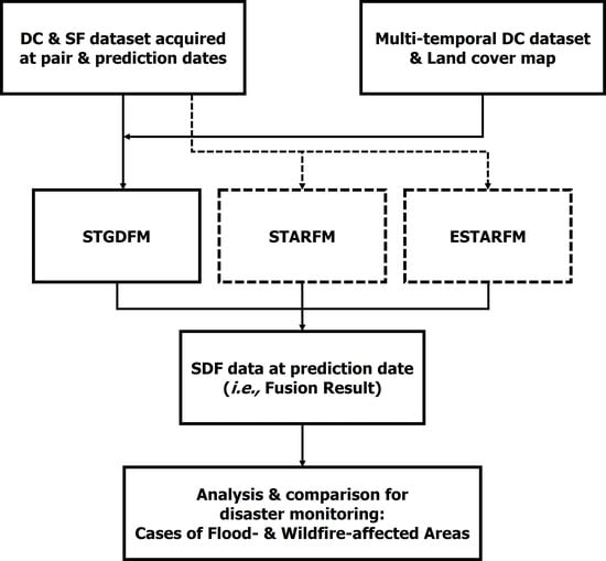
Based on this, this study assessed the applicability of STGDFM in disaster monitoring. To assess its explanatory capacity on the abrupt reflectance changes due to disasters, the study compared STGDFM and two other popular spatiotemporal data fusion models, STARFM and ESTARFM, and evaluated the results. The applicability assessment was conducted two case study areas affected by flood and wildfire. The near the Gwydir River Catchment located in Australia was selected as the study area of the Case of Flood-affected Area. In the Case of Flood-affected Area, the applicability assessment used simulation data using Landsat satellite images. The part of Nebraska state in the U.S. was selected as the study area of the Case of Wildfire-affected Area. Landsat and MODIS satellite images were used for the applicability assessment in the Case of Wildfire-affected Area.

2. Spatial Time Series Geostatistical/Deconvolution Fusion Model

This study supposes that the reflectances in the DC and SF data are $Z^C\left(v_i,t_d\right)$ and $Z^F\left(u_j,t_k\right)$, respectively. Here, the superscripts $C$ and $F$ refer to coarse-scale and fine-scale, and $v_i$ and $u_j$ are the $i$th and $j$th coarse-scale and fine-scale in the $N$th and $M$th coarse-scale and fine-scale pixels, respectively. Additionally, $t_d$ and $t_k$ refer to the acquisition date of the DC and SF data, respectively, and are $t_k\subseteq t_d$ because the DC data is more frequently acquired than the SF data. Furthermore, $t_k$ is the pair date considering the composition of the input data in the spatiotemporal data fusion. Accordingly, STGDFM predicts ${\widehat{Z}}^F\left(u_j,t_p\right)$, the DFS data, at the prediction date.

STGDFM first decomposes the predictive properties into trend and residual components [9]. Therefore, the DC data at the prediction date can be defined as follows:

$$Z^C\left(v_i,t_p\right)=m^C\left(v_i,t_p\right)+r^C\left(v_i,t_p\right)$$

(1)

where $m^C\left(v_i,t_p\right)$ and $r^C\left(v_i,t_p\right)$ refer to the trend component and the residual component in $t_p$, respectively. In the same context, ${\widehat{Z}}^F\left(u_j,t_p\right)$, the spatiotemporal data fusion result, is expressed as the sum of the trend and residual components estimated in the fine-scale location $t_p$.

$${\widehat{Z}}^F\left(u_j,t_p\right)={\widehat{m}}^F\left(u_j,t_p\right)+{\widehat{r}}^F\left(u_j,t_p\right)$$

(2)

where ${\widehat{m}}^F\left(u_j,t_p\right)$ and ${\widehat{r}}^F\left(u_j,t_p\right)$ refer to the trend and residual components estimated at the fine-scale location at $t_p$, respectively.

To estimate ${\widehat{m}}^F\left(u_j,t_p\right)$ from $m^C\left(v_i,t_p\right)$, STGDFM implements the spatial time series modelling and deconvolution matrix. Additionally, to estimate ${\widehat{r}}^F\left(u_j,t_p\right)$ from $r^C\left(v_i,t_p\right)$, it applies a geostatistics-based downscaling technique: area-to-point kriging (ATPK).

First, STGDFM applies a spatial time series modeling to quantify the temporal trend components from the multi-temporal DC data [22]. These temporal trend components refer to the quantification of the trend of the change of predictive properties over time. The multi-temporal DC data can be considered spatial time series that have time series values per pixel unit. Based on this, the temporal trend components are calculated at all coarse-scale pixel locations $v_i$ through spatial time series modeling. Spatial time series modeling calculates temporal trend components by estimating the relationship between the time series value at each coarse-scale pixel and the basis time series elements [9].

To consider the characteristics of land cover types, STGDFM defines the basis time series elements as the time series value per key land cover types of the target areas. For example, this time series value per land cover type means the calculation of the average value of all pixels in DC data corresponding to Class 1 by the acquisition date of the DC data. Further, STGDFM uses random forest, a non-parametric model, to define the relationship between the calculated basis time series elements and the time series value of each coarse-scale pixel [24]. Through the result of random forest, the temporal trend components based on the DC data are quantified.

The previously estimated temporal trend components are quantified in the spatial resolution of the DC data. Therefore, to estimate the trend components in the fine-scale resolution, STGDFM uses a deconvolution matrix. The deconvolution matrix defines the linear relation of the DC and SF data acquired from the pair date in matrix form [20]. Based on this, if there are DC and SF data acquired from $K$ number of pair dates, $K$ number of deconvolution matrices can be constructed. Because there are no true values of the SF data, the deconvolution matrix at $t_p$ is estimated by the weighted coupling of the deconvolution matrix constructed in the pair dates.

Here, the weighted value is calculated by the relationship between the temporal trend components quantified at the prediction date and the pair date. That is, the relationship between the quantified temporal trend components at the prediction date and in each pair date is calculated, and a higher weighted value is assigned to the deconvolution matrix constructed in the highly correlated pair date. Although correlation can be generally calculated in the whole research region, the global relationship assumes that the local variability is not considered, and a linear relationship appears constantly in the whole research region [25]. However, because the linear relationship can differ by region, STGDFM uses a regional linear relationship coefficient to calculate the weighting value, which is assigned to the deconvolution matrix. Thus, the weighted value assigned to the deconvolution matrix at each pair date is calculated, and the deconvolution matrix at the prediction date is estimated by the weighted coupling of the deconvolution matrix per pair date. Further, STGDFM estimates fine-scale trend components ${\widehat{m}}^F\left(u_j,t_p\right)$ by applying the estimated deconvolution matrix to the temporal trend components at the prediction date.

According to Equation (2), the predictive properties are not included in the trend component modeling, whereas the residual properties—that is, the residual components—are included. Therefore, to predict the spatiotemporal fusion result ${\widehat{Z}}^F\left(u_j,t_p\right)$, both the trend components and the residual components should be estimated simultaneously. To this end, STGDFM first calculates the coarse-scale residual components $r^C\left(v_i,t_p\right)$ at the prediction date. The coarse-scale residual components use the previously estimated fine-scale trend components ${\widehat{m}}^F\left(u_j,t_p\right)$. First, Gaussian kernel-based point spread function (PSF) is applied to the final-scale trend components to upscale the components to the coarse-scale resolution. Then, through the difference between the trend components upscaled by Equation (1) and the DC data acquired at $t_p$, the coarse-scale residual components are calculated. Next, to estimate the fine-scale residual components in Equation (2), STGDFM uses ATPK, a geostatistics-based downscaling technique [26]. The ATPK estimates the fine-scale residual components by the weighted linear coupling of the coarse-scale residual components, as shown in Equation (3):

$${\widehat{r}}^F\left(u_j,t_p\right)={\displaystyle \sum }_{i=1}^N{\lambda }_i\left(u_j\right)r^C\left(v_i,t_p\right)$$

(3)

where ${\lambda }_i\left(u_j\right)$ refers to the weighting value of ordinary kriging assigned to the $i$th coarse-scale residual components ($r^C\left(v_i,t_p\right))$ close to the predicted location ($u_j$). This weighting value can be calculated by the concept of block kriging [27].

Finally, STGDFM produces the spatiotemporal fusion result ${\widehat{Z}}^F\left(u_j,t_p\right)$ by summing the fine-scale residual components estimated by Equation (3) and the fine-scale trend components estimated through the spatial time series modeling and deconvolution matrix [9].

3. Experimental Design

3.1. Study Areas and Datasets

3.1.1. The Case of Flood-Affected Area

In this study, two types of disasters were selected as case studies: (1) Case of Flood-affected Area and (2) Case of Wildfire-affected Area (Figure 1). As shown in Figure 1a, the study area of the first case was near the Gwydir River Catchment, located in New South Wales, Australia. A large area of agricultural lands was flooded because of heavy rains from November to December 2004 [28,29]. An expanse of 320 km² (16 $\times$ 20 km²) including the flood-damaged areas was defined as the study area for this case.

An experiment was conducted using data simulated and generated from multi-temporal Landsat datasets. This only considered the difference in spatial resolution between Landsat and MODIS images, since MODIS and Landsat images have different spectral wavelengths and acquisition time. In the spatiotemporal data fusion, SF data are often upscaled to generate simulated DC data for construction of experimental data, which is used as input data. This is to easily construct a pair of DC and SF data, and these simulation data can be used as an alternative to real data (i.e., multiple sensor-based satellite images) when evaluating the performance of spatiotemporal data fusion. In the previous studies, from this point of view, the simulation data generated using SF data were used to evaluate the performance of spatio-temporal data fusion [9,20,30,31]. Likewise, this study used the simulation data generated from Landsat data as input data.

For this experiment, 12 cloud-free Landsat-5 TM images were collected from Earth Explorer (EE) of the U.S. Geological Survey (USGS); the acquisition dates of those are presented in

Table 1. Acquisition dates of dense time series data with a coarse-scale (i.e., DC data) generated original Landsat datasets for the Case of Flood-affected Area. The dates are listed in chronological order and the years are indicated only on the first and eighth dates. The underlined dates were assumed to be the dates when Landsat data used as sparse time series data with a fine-scale (i.e., SF data) were acquired, and these dates indicate the pair dates of DC and SF data. A bold underlined date indicates a prediction date.

No.	1	2	3	4
Date	16 April 2004	2 May	5 July	22 August
No.	5	6	7	8
Date	25 October	26 November	28 December	13 January 2005
No.	9	10	11	12
Date	29 January	14 February	2 March	3 April

. The prediction date for the flood-affected area was defined as 26 November 2004. Then, 2 May 2004 and 14 February 2005—before and after the prediction date—were defined as pair dates (Table 1). Considering Landsat images acquired at a low frequency (e.g., one- or two-month) (Table 1) for using simulation data, however, the experiment was conducted based on an assumption that the changes in reflectance were not large between the acquisition dates of Landsat images.

For generating the simulation data, the acquired Landsat images upscaled to 240 m was used as DC data, which were upscaled by applying the Gaussian PSF. The upscaled Landsat images (i.e., DC data) were considered as MODIS images provided daily at a 250 m spatial resolution, which are MOD09GQ products [32]. This study applied the rectangular PSF, which is mainly applied to scale conversion in remote sensing data [9,20,30]. Specifically, in the upscaling using rectangular PSF, a coarse-scale pixel value is determined through a weighted combination of fine-scale pixels included in the coarse-scale pixel. Here, a scale factor must be defined, which is defined as the square root value of the fine-scale pixels included in the coarse-scale pixel. Regarding this, the scale factor is a positive integer value, in this study, the scale factor is defined as 8. Therefore, the spatial resolution of original MODIS data is 250 m, but by defining the scale factor as 8, the spatial resolution of MODIS data was considered to be 240 m. In a real case using multi-sensor satellite images, also, the acquisition date of SF data is more sparsely than that of DC data. Considering this situation, Landsat images, which are SF data, were assumed to be acquired at only the pair dates. Based on this, the composition of DC and SF data used in the Case of Flood-affected Area is shown in Table 1.

This study applied the spatiotemporal data fusion for red and near-infrared (NIR) channels. When mapping areas affected by flood using remote sensing data, in particular satellite images, normalized difference vegetation index (NDVI) is commonly used as a biophysical parameter [33,34]. Considering this, red and NIR bands, which are input channels for calculating NDVI, were selected as target reflectance channels for spatiotemporal data fusion. Based on this, Figure 2 shows DC and SF data after preprocessing in red and NIR channels.

In addition to DC and SF data, STGDFM uses a land-cover map as the input data. For this, a land-cover map provided by Emelyanova et al. [28] was used. The land-cover map used in the Case of the Flood-affected Area is shown in Figure 1a, which includes the damage areas of flood (i.e., flooded area). The land-cover map was provided at a spatial resolution of 500 m, but was converted to a spatial resolution of 240 m using the nearest neighboring interpolation method to match the spatial resolution with the DC data in the application of STGDFM.

Finally, the input data used in the Case of Flood-affected Areas are summarized as follows: Landsat-5 TM data were used as SF data, and the spatial resolution was defined as 30 m which are the same as the resolution of the original Landsat data. As DC data, the result of upscaling Landsat-5 TM data to 240 m was used (Figure 2). Additionally, the land-cover map converted to the spatial resolution of 240 m was used as input data for STGDFM.

3.1.2. The Case of Wildfire-Affected Area

The study area for the Case of the Wildfire-affected Area was selected as Nebraska state in the U.S. This area was damaged by a wildfire on 3 August 2002, which affected an area of 6463 ha according to Monitoring Trends in Burn Severity released by the USGS [35]. Thus, an expanse of 256 km² (16 $\times$ 16 km²) including the damaged areas affected by wildfire was defined as the case study area (Figure 1b).

In the Case of Wildfire-affected Area, MODIS and Landsat data were used for DC and SF data, respectively. Unlike the Case of Flood-affected Area, for which simulated data were used, different satellite images were used to assess applicability based on actual satellite images. As for DC data, MODIS Terra-based MOD09GQ products were used. As has been explained in the Case of Flood-affected Area, the spatial resolution of MODIS data was resampled to 240 m by the nearest neighboring interpolation method. Landsat-7 ETM+ was used as SF data, but the images taken before the failure of the scan line correction device were used since the target date is 2002. As in the Case of Flood-affected Area, NDVI is commonly used as a biophysical parameter in the mapping areas affected by wildfire [36,37]. For this reason, the reflectance data in red and NIR channels of MODIS and Landsat data were used in this case.

Considering the growth cycle of cropland and grass, the main land coverage types in the case region, the acquisition date of the data was set from April to October 2002, in which 19 MODIS data and 3 Landsat data without cloud interference were acquired. In particular, the images in August after the wildfire and the Landsat images taken in June and September, before and after the wildfire, were acquired. This study used the Landsat images acquired on 14 August as the true value of the data and the MODIS and Landsat images acquired on 11 June and 15 September as the pair data (

Table 2. Acquisition dates of MODIS datasets used as DC data for the Case of Wildfire-affected Area. The dates are listed in chronological order and the year is indicated only on the first date. The underlined dates indicate the pair dates of MODIS and Landsat datasets used as DC and SF data, respectively. A bold underlined date indicates a prediction date.

No.	1	2	3	4
Date	1 April 2002	17 April	24 April	17 May
No.	5	6	7	8
Date	1 June	11 June	25 June	29 June
No.	9	10	11	12
Date	9 July	18 July	25 July	7 August
No.	13	14	15	16
Date	14 August	31 August	6 September	15 September
No.	17	18	19
Date	20 September	4 October	13 October

). Shown in Figure 3 are the MODIS and Landsat data pre-processed in red and NIR channels.

As the land-cover map, Cropland Data Layer (CDL), provided by the USDA NASS, was used [38]. This study reassigned CDL data containing the 256 land-cover types into the main types in the target area, such as corn, soybean, hay/grain, and grass (Figure 1b). Since CDL data is provided at 30 m, for the application of STGDFM, CDL data were upscaled to 240 m, which is the spatial resolution of the DC data. For this, the fraction of land-cover types included in a coarse-scale pixel was calculated, and a land-cover type which is the highest fraction was assigned to the corresponding the coarse-scale pixel.

The input data used in the Case of Wildfire-affected Areas are summarized as follows: MODIS MOD09GQ data were used as DC data, and the spatial resolution was defined as 240 m. Landsat-7 ETM+ data, then, were used as SF data, of which spatial resolution was set to 30 m (i.e., the resolution of the original Landsat data) (Figure 3). Lastly, the CDL data was used as the land-cover map, and the spatial resolution of CDL was converted to 240 m.

3.2. Method

Figure 4 presents a flowchart that depicts the way this study was carried out and the resources used. The study applied STGDFM, STARFM, and ESTARFM to the Case of Flood-affected Area using simulation data and the Case of Wildfire-affected Area using MODIS and Landsat data. STARFM and ESTARFM are representative spatiotemporal data fusion models with proven predictive performance in various studies [14,28,39,40]. Further, unlike STGDFM, which models the reflectance changes using time series DC data, STARFM and ESTARFM assume for reflectance changes between the prediction date and the pair dates [18,19]. When explaining the changes in reflectance due to the disaster, this study confirmed whether these assumptions could be applied, unlike modeling the changes in reflectance. Consequently, these three models with different characteristics were compared in prediction performance the abrupt reflectance changes due to disasters.

To implement STARFM and ESTARFM, the model’s parameters must be defined. This study defined the model parameters for each case through the preliminary experiment. The main parameters required for the application of these two models are the size of the search window and the number of classification items. Here, the number of classification items was identically defined as the number of classification items of the land coverage type used in STGDFM. Additionally, the size of the search window was set to 12 and 15 for each case in consideration of the spatial resolution of Landsat data and the spatial size of the target region.

This study conducted qualitative and quantitative assessments, to compare the results of STARFM, ESTARFM, and STGDFM. True SF data acquired at the prediction date were used as the validation data, which were Landsat data acquired at 26 November 2004 and 14 August 2002 in the Cases of Flood- and Wildfire-affected Areas, respectively. The qualitative assessment visually compared the true values of the SF data and the results of the three fusion models. The quantitative assessment compared the results by calculating the amounts of four validation indices. First, to assess prediction accuracy, the study calculated the mean absolute error (MAE). Targeting the fusion results of the three models, the MAE based on the true values of the SF data acquired at each prediction date was calculated by Equation (4):

$$\mathrm{MAE}=\frac{1}{M}{\displaystyle \sum }_{j=1}^M|{\widehat{Z}}^F\left(u_j,t_p\right)-Z^F\left(u_j,t_p\right)|$$

(4)

The root mean square error (RMSE) was selected as second validation indices. As with MAE, the RMSE of the fusion result was calculated using the SF data acquired at each prediction date, as shown in Equation (5):

$$\mathrm{RMSE}=\sqrt{\frac{1}{M}{\displaystyle \sum }_{j=1}^M{({\widehat{Z}}^F\left(u_j,t_p\right)-Z^F\left(u_j,t_p\right))}^2}$$

(5)

Next, the study used the structural similarity index measure (SSIM) that can quantitatively compare spatial similarity. To evaluate the similarity between two images, Wang et al. [37] developed SSIM to calculate spatial similarity quantitatively by using the mean value, standard deviation, and covariance of the two images. While SSIM can be calculated with the global statistics of the image, Wang et al. [41] calculated it locally by defining the search window. In other words, SSIM is calculated within each search window, and the SSIM value calculated at the central pixel of the search window is assigned to calculate the SSIM value of all pixels, as shown in Equations (6)–(9):

$$\mathrm{SSIM}(\frac{1}{W},\frac{1}{W},t_p)=\frac{(2{\mu }_Z{\mu }_{\widehat{Z}}+C_1)(2{\sigma }_{Z\widehat{Z}}+C_2)}{({\mu }_Z{}^2+{\mu }_{\widehat{Z}}{}^2+C_1)({\sigma }_Z{}^2+{\sigma }_{\widehat{Z}}{}^2+C_2)}$$

(6)

$${\mu }_Z=\frac{1}{L}{\displaystyle \sum }_{l=1}^L{Z}^F\left(u_l,t_p\right)$$

(7)

$${\sigma }_Z=\sqrt{\frac{1}{L}{\displaystyle \sum }_{l=1}^L(Z^F\left(u_l,t_p\right)-{\mu }_Z)}$$

(8)

$${\sigma }_{Z\widehat{Z}}=\frac{1}{L}{\displaystyle \sum }_{l=1}^L\left\{(Z^F\left(u_l,t_p\right)-{\mu }_Z)({\widehat{Z}}^F\left(u_l,t_p\right)-{\mu }_{\widehat{Z}})\right\}$$

(9)

where $W$ means the window size and $L$ means the number of pixels including within the window. Additionally, $C_1$ and $C_2$ are the constants calculated by ${\left(0.01\times ℒ\right)}^2$ and ${\left(0.03\times ℒ\right)}^2$, respectively. Here, $ℒ$ means a dynamic range value. Since reflectance has a value from 0 to 1, $ℒ$ is defined as 1 in this study.

This study used a mean SSIM index, as the quantitative assessment statistic. The mean SSIM index has a value between 0 and 1, and the closer it is to 1, the higher is the spatial similarity between the two images.

As the fourth evaluation index, this study calculated and compared the R-squared (R²) value. The R² has a value between 0 and 1, which can be calculated by Equation (10). The closer R² value is to 1, the higher correlation between the fusion result and true SF data.

$${\mathrm{R}}^2\left(t_p\right)=\frac{{{\displaystyle \sum }}_{j=1}^M({\widehat{Z}}^F\left(u_j,t_p\right)-\overline{Z^F}\left(t_p\right))}{{{\displaystyle \sum }}_{j=1}^M({\mathrm{Z}}^F\left(u_j,t_p\right)-\overline{Z^F}\left(t_p\right))}$$

(10)

where $\overline{Z^F}\left(t_p\right)$ means the mean value of true SF data acquired at the prediction date ($t_p$).

Further, to compare the damage detection results by each spatial-temporal fusion model in the comparative analysis of the results, the study conducted both global and local comparisons. Here, global comparison refers to the qualitative and quantitative comparisons of the true values and prediction results targeting the whole research region. The local comparison refers to the comparison of the true values and prediction results targeting the region where damage by disaster has been detected. For the local comparison, the study used the vector data obtained in the flood and wildfire damaged regions for each case.

4. Results

4.1. Case of Flood-Affected Area

First, the study visually compared the true SF data acquired on 26 November 2004, the prediction date, and the results of the three fusion models. As for the fusion results in the red channel, shown in Figure 5, all three fusion models were verified to have low reflectance values in the flood-damaged region. However, if the local variance in the flood-damaged region is compared, a higher reflectance value was predicted in the application of STARFM and ESTARFM. STGDFM produced its fusion result with a spatial trend like that of the true SF data.

Such a result can also be noted in Figure 6, which is an enlarged comparison of the flood-damaged region. The true SF data showed low reflectance values due to flood damage. It was shown that STGDFM predicted the low reflectance values of damage by flood at a closer level to the true SF data than to STARFM and ESTARFM. STARFM reflected the low reflectance values in the DC data on the prediction date, but it did not reflect the detailed patterns of the true SF data. Such a trend was also shown in ESTARFM; in particular, the fusion result in ESTARFM and the noise patterns identical to Subarea A in Figure 6 were verified.

While the true SF data observed the shape of rivers, as shown in Figure 6, the results of three fusion models were not reflected this shape. Three fusion models combine the local variations of SF data acquired at the pair dates to predict the local variations at the prediction date. In this case, however, the local variations including the shape of rivers were not observed in the SF data acquired at two pair dates. Therefore, this is considered that three fusion models failed to capture the shape of rivers in the results. In order to predict the local variations well, SF data with local variations similar to true values should be used as the pair data. However, it is difficult to obtain SF data at the desired date in terms of availability of optical satellite images. Although multiple sensor-based satellite images can be used as SF data, the relationship between DC and SF data should be defined differently for each sensor. If the multiple sensor-based satellite images are used as SF data, it is necessary to consider how to combine the sensor-based relationships between DC and SF data in spatiotemporal fusion.

Figure 7 presents the three spatial-temporal fusion results produced in the NIR channel and the true SF data. By visually comparing the three fusion results in the NIR channel, ESTARFM showed a fusion result higher than the true SF data in the flood-damaged region (over-estimated). STGDFM and STARFM showed a fusion result similar to the true SF data. However, when the fusion results of STGDFM and STARFM were expanded and compared, it was found that STARFM could not reflect the detailed patterns in Subarea A of Figure 8. Additionally, when STGDFM and STARFM were compared with ESTARFM, the latter showed the fusion result with a different spatial trend than the true SF data. In contrast, STGDFM reflected the low reflectance values well—in particular, the local variations in the true SF data.

Next, the study performed an accuracy assessment based on the spatiotemporal fusion results produced in red and NIR channels (

Table 3. Quantitative evaluation indices of three spatiotemporal data fusion results in the Case of Flood-affected Area. Local statistics refer to the validation statistics calculated only in flooded areas. The best performance is highlighted with underlining and bold font type.

Channel	Statistics		STGDFM	STARFM	ESTARFM
Red Channel	Global Statistics	MAE	0.0089	0.0081	0.0097
		RMSE	0.0118	0.0114	0.0136
		SSIM	0.916	0.902	0.908
		R2	0.874	0.852	0.823
	Local Statistics	MAE	0.0088	0.0086	0.0097
		RMSE	0.0122	0.0118	0.0134
		SSIM	0.911	0.892	0.885
		R2	0.872	0.869	0.832
NIR Channel	Global Statistics	MAE	0.0132	0.0137	0.0154
		RMSE	0.0192	0.0196	0.0200
		SSIM	0.890	0.889	0.886
		R2	0.836	0.822	0.807
	Local Statistics	MAE	0.0129	0.0133	0.0173
		RMSE	0.0189	0.0208	0.0239
		SSIM	0.894	0.891	0.878
		R2	0.838	0.834	0.832

). The accuracy assessment showed a result similar to that of visual verification, and the prediction performance of STGDFM was generally higher than that of STARFM or ESTARFM. However, when the MAE and RMSE values were compared in the red channel, STARFM showed lower MAE and RMSE values than STGDFM. It may be that STARFM reflected well the fusion result with a low reflectance value by using the DC data at the prediction date, which resulted in low MAE and RMSE values (Table 3). Although STARFM showed lower MAE and RMSE values than STGDFM, SSIM and R² values of STARFM (SSIM: 0.892, R²: 0.869) were lower than those of STGDFM (SSIM: 0.911, R²: 0.872). STARFM converts the spatial resolution of DC data into spatial resolution of SF data by applying bilinear interpolation, thus DC data with smoothed patterns were input for STARFM [18]. Particularly, STARFM showed limitations in explaining local variations by assigning high weights to DC data with smoothed patterns acquired at the prediction date. As a result, when compared to STGDFM, STARFM’s similarity to the true SF data was lower. The fusion results of STGDFM and STARFM showed similar patterns in the flood-affected areas, whereas ESTARFM fusion result showed significantly different patterns with true SF data (Figure 7 and Figure 8). Likewise, ESTARFM showed the lowest prediction performance among the three models with highest error measurement indices and lowest similarity indices in both red and NIR channels (Table 3).

On the other hand, the difference between the evaluation indices of STGDFM and STARFM does not seem significant, in terms of the absolute values. However, this difference may lead to different results in remote sensing applications. For this reason, even the small difference of this extent was regarded as a significant improvement in previous studies [19,20,39,42].

4.2. The Case of Wildfire-Affected Area

Next, the results of spatial-temporal fusion applied to the Case of Wildfire-affected Area were compared. First, the spatial-temporal fusion results produced in the red channel and the true SF data (i.e., Landsat data acquired at a prediction date) were visually compared (Figure 9). Further, all three models were generally shown to produce fusion results with a spatial trend similar to the true Landsat data. As shown in Figure 9, it is determined that this is because in the red channel, the reflectance value due to wildfire is not significant.

In all three fusion results, the global spatial pattern was similar to that of the true SF data, but the local variation showed different trends (Figure 9 and Figure 10). In Subarea A, a region with relatively lower wildfire damage, shows a higher reflectance value than the surrounding region in the true SF data. Such a trend was seen in STGDFM but not in STARFM and ESTARFM. Additionally, Subarea B showed a low reflectance value in the true SF data. When compared with STARFM and ESTARFM, STGDFM predicted in the fusion result a low reflectance value similar to the true SF data.

Figure 11 shows the comparison of the spatiotemporal data fusion results produced in the red and NIR channels. The result shows that the ESTARFM fusion result predicted a higher reflectance value than the Landsat data, which was observed to have a lower reflectance value due to wildfire damage. However, when compared to the true Landsat data, the fusion results from STGDFM and STARFM predicted a global spatial pattern similar to that of the true value data.

As opposed to the global spatial pattern, the fusion results of STGDFM and STARFM show the difference in the local variation. As shown in Figure 12, in Subareas A and B, which are the expanded areas of the wildfire-affected regions, STGDFM explains the local variation more like the trend in the true Landsat data than STARFM. The fusion result of STARFM showed locally smoothed patterns when compared to the true Landsat data. Further, the fusion result of ESTARFM showed significantly different local variations from the true Landsat data.

In addition to the visual verification, the study quantitatively compared the prediction performance of the fusion results (

Table 4. Quantitative evaluation indices of three spatiotemporal data fusion results in the Case of Wildfire-affected Area. Local statistics refer to the validation statistics calculated only in wildfire affected areas. The best performance is highlighted with underlining and bold font type.

Channel	Statistics		STGDFM	STARFM	ESTARFM
Red Channel	Global Statistics	MAE	0.0103	0.0108	0.0116
		RMSE	0.0148	0.0149	0.0165
		SSIM	0.945	0.925	0.927
		R2	0.900	0.895	0.872
	Local Statistics	MAE	0.0091	0.0094	0.0105
		RMSE	0.0120	0.0121	0.0143
		SSIM	0.979	0.967	0.938
		R2	0.775	0.769	0.700
NIR Channel	Global Statistics	MAE	0.0214	0.0207	0.0261
		RMSE	0.0333	0.0318	0.0412
		SSIM	0.950	0.911	0.900
		R2	0.916	0.910	0.860
	Local Statistics	MAE	0.0144	0.0144	0.0199
		RMSE	0.0190	0.0192	0.0261
		SSIM	0.949	0.921	0.917
		R2	0.760	0.742	0.717

). Similar to the Case of Flood-affected Areas, STGDFM generally showed the highest prediction performance among the three fusion models. Specifically, in the local statistics of both red and NIR channels, the lowest RMSE (red channel: 0.0120, NIR channel: 0.0190) and the highest SSIM (red channel: 0.979, NIR channel: 0.949) were presented in the results of STGDFM. Although the lowest MAE and RMSE values in the global statistics of NIR channel were presented in the result of STARFM, the similarity indices (i.e., SSIM and R²) of STARFM were lower than those of STGDFM. This is considered that the effect of smoothed patterns presented in the fusion results of STARFM (Figure 12). As mentioned in the Case of flood-affected Areas, since STARFM assigned a high weight to DC data with smoothed patterns acquired at the prediction date, the fusion result of STARFM included the smoothed patterns compared with the results of STGDFM and ESTARFM. On the other hand, ESTARFM showed the highest error measurement indices (i.e., MAE and RMSE) and the lowest similarity indices. Particularly, in the NIR channel, it was found that ESTARFM showed a significant difference in the prediction performance compared to STGDFM and STARFM. These results are discussed in Discussion.

5. Discussion

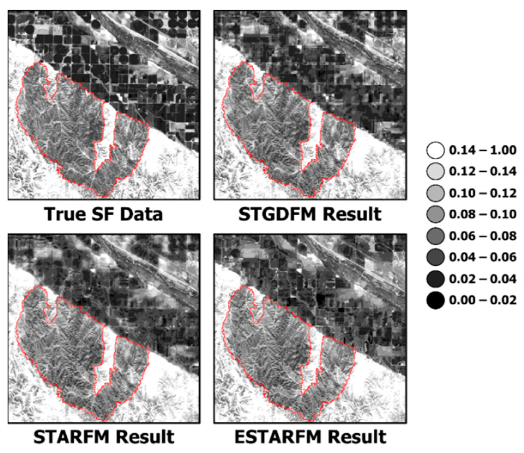
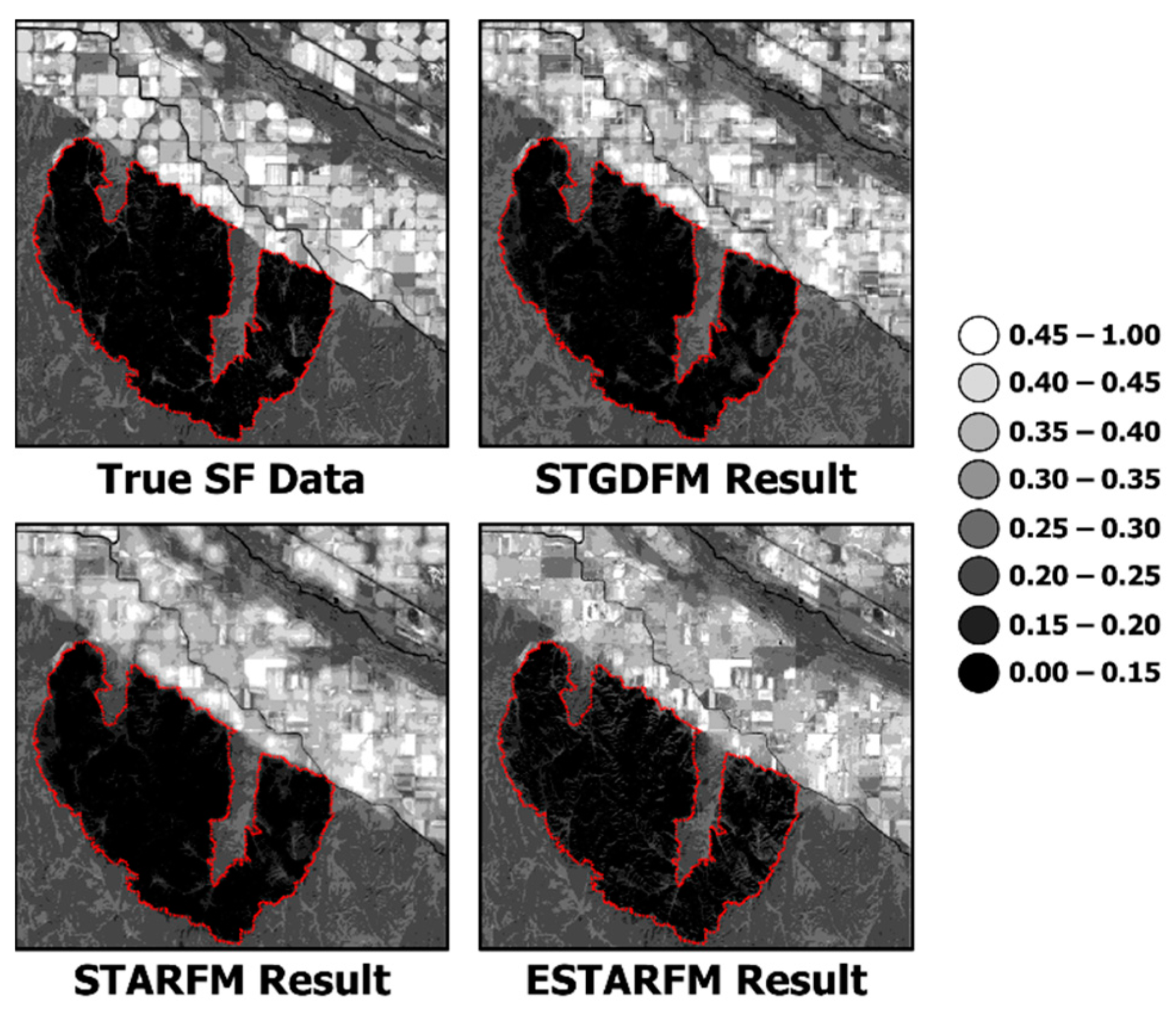
The summary of the key results of this study are as follows: (1) The ESTARFM fusion result showed poor prediction performance in the reflectance changes in the damaged region and the period, as opposed to the Landsat data from the prediction date. (2) The STARFM fusion result showed a locally smoothed pattern in contrast to the application results of the other two models. (3) When compared to the fusion results of STARFM and ESTARFM, the fusion result of STGDFM showed a higher prediction performance. This section presents the analysis of the results.

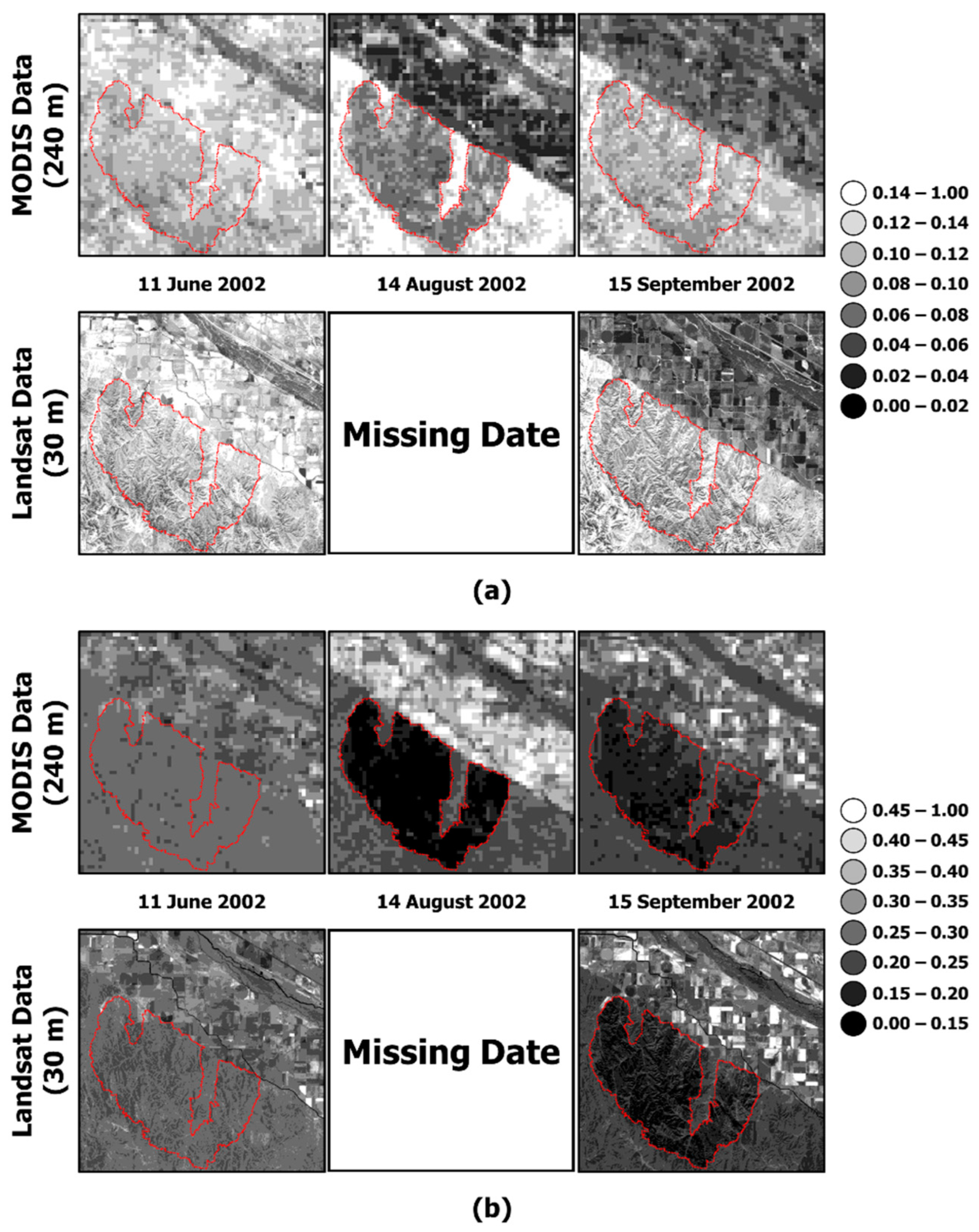
This study constructed the DC and SF data acquired before and after disaster as pair data and used them as input data to detect the region damaged by disaster (Figure 2 and Figure 3). The NIR channel data that showed a significant amount of the reflectance changes due to disaster (Figure 2b and Figure 3b) showed that there were huge reflectance changes between the pair dates and the prediction date. In particular, such reflectance changes were considerable in the first pair date, the time before the disaster, and the prediction date. However, ESTARFM assumes that reflectance changes linearly between the pair dates and the prediction date [19]. Therefore, if there is a considerable change of reflectance between the prediction date and the pair dates due to disaster, it is difficult to assume that reflectance changes linearly. As such, the prediction performance of ESTARFM was the poorest among the three models. The previous studies also reported this interpretation in Xue et al. [20].

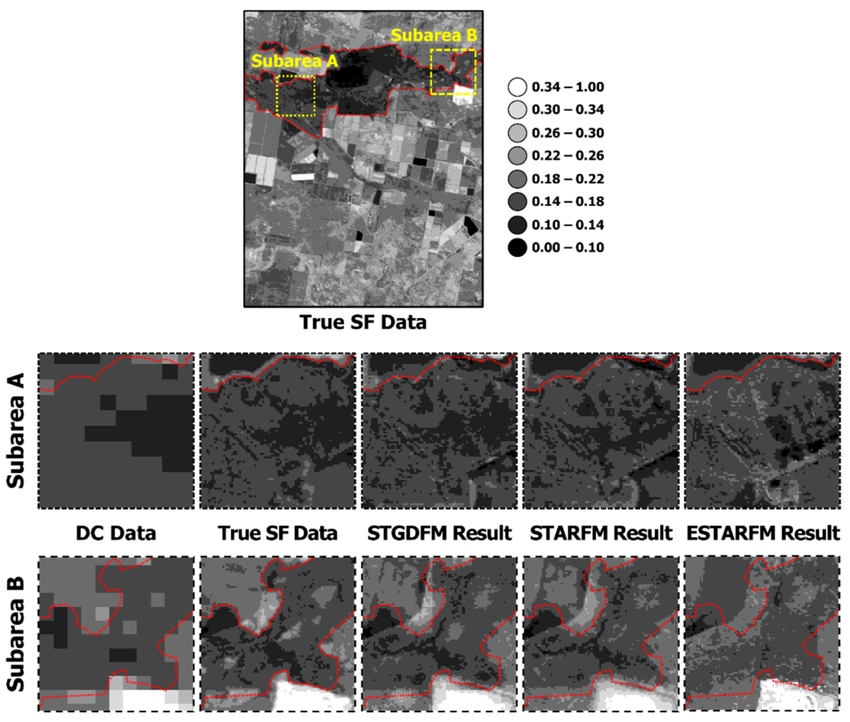
As opposed to ESTARFM, STARFM assumes that the changes observed in the DC data are maintained in the fine-scale data [18]. Therefore, if damage by disaster was observed in the DC data acquired in the prediction date, as shown in Figure 3, such data can be reflected onto the fusion result to explain the reflectance changes due to a disaster. As such, it is determined that STARFM showed a relatively more improved prediction performance, compared to ESTARFM. However, the fusion result of STARFM showed a smoothed pattern; in particular, the region with marked damage by wildfire, as shown in Figure 12, did not reflect the local variations observed in the true SF data.

This is because such a result does not reflect the difference in the spatial resolution between the DC and SF data in the process of coupling the reflectance changes observed in the DC data according to STARFM’s assumption. Further, STARFM uses DC data converted into the spatial resolution of SF data as input data by applying bilinear interpolation. The DC data with the converted spatial resolution presents a smoothed pattern. Here, to explain the reflectance changes due to disaster, STARFM assigns a high weighting value to the DC data with the converted spatial resolution acquired on the prediction date. As a result, the effect of the DC data with smoothed patterns is largely reflected in the fusion result of STARFM, which showed limitations in explaining local variations. These results are conspicuous in Figure 12, which enlarges the wildfire-affected areas. This means that to couple the reflectance changes observed in the DC data to the fusion result, the difference in the spatial resolution between the DC and SF data should be considered.

Next, the study analyzed the result of STGDFM, which showed a relatively higher predictive performance with its fusion result. As STGDFM is based on the decomposition of the components into the trend and residual components [9], the study examined the trend and residual components, the intermediate result of STGDFM by each case (Figure 13 and Figure 14). To analyze the effect of the residual components on the fusion result of STGDFM, this study compared the absolute value of the residual components, where the larger the absolute value of the residual components, the greater the effect of the residual.

As show in Figure 13 and Figure 14, the effect of the residual components was higher in the red channel than in the NIR channel. Here, the large influence of the residual component means that the effect of the DC data acquired on the prediction date was highly reflected in the STGDFM fusion result explaining the reflectance changes due to the disaster. The reason for a large effect of the residual components in the NIR channel is that the main land coverage in two cases was vegetation (Figure 1). Further, with flooding and wildfire, there was a change in the proportion of vegetation coverage, a key land coverage type in the two regions. Vegetation shows sensitive responses to reflectance changes in the NIR channel; as a result, the effect of the residual components increased in STGDFM to explain the reflectance changes due to disaster in vegetation coverage. In particular, the effect of the residual components was higher in the Case of Flood-affected Area, whereas no reflectance change resulting from disaster is observed in a date different from the prediction date (Figure 2b and Figure 13b).

The case of Wildfire-affected Area explains the reflectance changes due to wildfire not only with the residual components but also with the trend components (Figure 14). Specifically, the effect of the trend components was shown to be considerably applied in the lower right corner of the wildfire-damaged region. As in Figure 3, this is because damage by wildfire was also observed in the DC and SF data acquired after the wildfire. In other words, damage by wildfire was observed in dates other than the prediction date, and the changes in reflectance observed here could be explained in the fusion result with the trend components.

Meanwhile, the large effect of the residual components in STGDFM mean that the influence of DC data acquired on the prediction date was greatly reflected in the fusion result. While this is similar to STARFM where a high-weighing value is assigned to the DC data acquired on the prediction date, the smoothing pattern observed in the fusion result of STARFM did not occur in that of STGDFM. Thus, STGDFM explained the local variations of the SF data in the trend components by using the deconvolution matrix, which was then coupled with residual components to produce the fusion result in the spatial pattern similar to the true SF data.

In summary, STGDFM explained the reflectance changes due to disaster through the trend components and the residual components. In particular, its explanatory power for the abrupt reflectance changes due to disaster could be improved by reflecting the large effect of the residual components for the prediction date. Furthermore, STGDFM combines with the trend components the local variations of the SF data acquired in the pair dates based on the deconvolution matrix. In this way, STGDFM could produce fusion results with the true SF data and fine-scale spatial similarity (i.e., higher SSIM values) compared to STARFM and ESTARFM.

6. Conclusions

This study assessed the applicability of the spatiotemporal data fusion for the detection of regions damaged by disaster. To this end, the performance of detecting regions damaged by disaster was analyzed using spatiotemporal fusion results. In particular, the study applied three spatiotemporal data fusion models to detect the region damaged by disaster and compared and analyzed their performance. The summary of the analysis is as follows: (1) ESTARFM assumes that the reflectance changes linearly between the pair date and the prediction date; thus, its explanatory power for the reflectance changes due to disaster was relatively poor. (2) STARFM assumes that the reflectance changes observed in the DC data are maintained in the SF data; thus, it was limited in explaining the detailed variations of the reflectance changes. (3) STGDFM was able to show the highest prediction performance among the three models as it explained the reflectance change due to disaster with the residual components and the detailed variations of the reflectance changes with the trend components. Based on these results, STGDFM is expected to be useful only if DC data is acquired in the detection of regions damaged due to disaster.

The experimental results showed that the spatiotemporal data fusion can effectively produce synthetic satellite images with high spatial and temporal resolutions. For monitoring of disasters such as flood, wildfire, and forest landslide, fine-scale time series satellite images should be constructed quickly. The government or local governments can use these data to yield the scale and damage of disasters and to establish prevention measures in advance. In this respect, spatiotemporal data fusion methods need to be continuously enhanced. Even if this study compared and analyzed the performance of the three spatiotemporal data fusion models in disaster monitoring, there are still issues to be discussed or improved. For example, unlike the reflectance changes due to disasters, in order to predict the changes in reflectance due to climate change, the long time series satellite images should be used. Consequently, the geostatistical spatial time series modeling applied in STGDFM can capture the temporal trends from the long time series satellite images. However, since reflectance changes due to climate change generally appear in large areas, the difference in spatial resolution of DC and SF data may increase depending on the coverage area. As the difference in spatial resolution between DC and SF data increases, the noise patterns such as block artifacts can become more pronounced in the result of STGDFM. To reduce these noise patterns, stepwise STGDFM can be applied. That is, instead of directly converting DC data into spatial resolution of SF data, the spatial resolution is converted stepwise to finally generate SDF data. Therefore, in the future study, the prediction performance of STGDFM for reflectance changes due to climate change will be evaluated, and STGDFM will be improved to be applicable on a large scale.

References

1. Ghafffarian, S.; Emtehani, S. Monitoring urban deprived areas with remote sensing and machine learning in case of disaster recovery. Climate 2021, 9, 58. [Google Scholar] [CrossRef]
2. Antzoulatos, G.; Kouloglou, I.-O.; Bakratsas, M.; Moumtzidou, A.; Gialampoukidis, I.; Karakostas, A.; Lombardo, F.; Fiorin, R.; Norbiato, D.; Ferri, M.; et al. Flood hazard and risk mapping by applying an explainable machine learning framework using satellite imagery and GIS data. Sustainability 2022, 14, 3251. [Google Scholar] [CrossRef]
3. Provost, F.; Michéa, D.; Malet, J.-P.; Boissier, E.; Pointal, E.; Stumpf, A.; Pacini, F.; Doin, M.-P.; Lacroix, P.; Proy, C.; et al. Terrain deformation measurements from optical satellite imagery: The MPIC-OPT processing services for geohazards monitoring. Remote Sens. Environ. 2022, 274, 112949. [Google Scholar] [CrossRef]
4. Hasanlou, M.; Shah-Hosseini, R.; Seydi, S.T.; Karimzadeh, S.; Matsuoka, M. Earthquake damage region detection by multitemporal coherence map analysis of radar and multispectral imagery. Remote Sens. 2021, 13, 1195. [Google Scholar] [CrossRef]
5. Chen, C.; Fu, J.; Gai, Y.; Li, J.; Chen, L.; Mantravadi, V.S.; Tan, A. Damaged bridges over water: Using high-spatial-resolution remote-sensing images for recognition, detection, and assessment. IEEE Geosci. Remote Sens. Mag. 2018, 6, 69–85. [Google Scholar] [CrossRef]
6. Wu, C.; Zhang, F.; Xia, J.; Xu, Y.; Li, G.; Xie, J.; Du, Z.; Liu, R. Building damage detection using U-Net with attention mechanism from pre- and post-disaster remote sensing datasets. Remote Sens. 2021, 13, 905. [Google Scholar] [CrossRef]
7. Belgiu, M.; Stein, A. Spatiotemporal image fusion in remote sensing. Remote Sens. 2019, 11, 818. [Google Scholar] [CrossRef] [Green Version]
8. Ghamisi, P.; Rasti, B.; Yokoya, N.; Wang, Q.; Höfle, B.; Bruzzone, L.; Bovolo, F.; Chi, M.; Anders, K.; Gloaguen, R.; et al. Multisource and multitemporal data fusion in remote sensing: A comprehensive review of the state of the art. IEEE Geosci. Remote Sens. Mag. 2019, 7, 6–39. [Google Scholar] [CrossRef] [Green Version]
9. Kim, Y.; Kyriakidis, P.C.; Park, N.-W. A cross-resolution, spatiotemporal geostatistical fusion model for combining satellite image time-series of different spatial and temporal resolutions. Remote Sens. 2020, 12, 1553. [Google Scholar] [CrossRef]
10. Eva, H.; Lambin, E.F. Fires and land-cover change in the tropics: A remote sensing analysis at the landscape scale. J. Biogeogr. 2000, 27, 765–776. [Google Scholar] [CrossRef]
11. Lupo, F.; Reginster, I.; Lambin, E.F. Monitoring land-cover changes in West Africa with SPOT vegetation: Impact of natural disasters in 1998–1999. Int. J. Remote Sens. 2001, 22, 2633–2639. [Google Scholar] [CrossRef]
12. Chen, L.; Guo, Z.; Yin, K.; Shrestha, D.P.; Jin, S. The influence of land use and land cover change on landslide susceptibility: A case study in Zhushan Town, Xuan’en County (Hubei, China). Nat. Hazards Earth Syst. Sci. 2019, 19, 2207–2228. [Google Scholar] [CrossRef] [Green Version]
13. Luo, D.; Goodin, D.G.; Caldas, M.M. Spatial-temporal analysis of land cover change at the Bento Rodrigues Dam disaster area using machine learning techniques. Remote Sens. 2019, 11, 2548. [Google Scholar] [CrossRef] [Green Version]
14. Zhang, F.; Zhu, X.; Liu, D. Blending MODIS and Landsat images for urban flood mapping. Int. J. Remote Sens. 2014, 35, 3237–3253. [Google Scholar] [CrossRef]
15. Zhong, D.; Zhou, F. Improvement of clustering methods for modelling abrupt land surface changes in satellite image fusions. Remote Sens. 2019, 11, 1759. [Google Scholar] [CrossRef] [Green Version]
16. Li, X.; Foody, G.M.; Boyd, D.S.; Ge, Y.; Zhang, Y.; Du, Y.; Ling, F. SFSDAF: An enhanced FSDAF that incorporates sub-pixel class fraction change information for spatio-temporal image fusion. Remote Sens. Environ. 2020, 237, 111537. [Google Scholar] [CrossRef]
17. Miura, T.; Nagai, S. Landslide detection with himawari-8 geostationary satellite data: A case study of a torrential rain event in Kyusu, Japan. Remote Sens. 2020, 12, 1734. [Google Scholar] [CrossRef]
18. Gao, F.; Masek, J.; Schwaller, M.; Hall, F. On the blending of the Landsat and MODIS surface reflectance: Predicting daily Landsat surface reflectance. IEEE Trans. Geosci. Remote Sens. 2006, 44, 2207–2218. [Google Scholar]
19. Zhu, X.; Chen, J.; Gao, F.; Chen, X.; Masek, J.G. An enhanced spatial and temporal adaptive reflectance fusion model for complex heterogeneous regions. Remote Sens. Environ. 2010, 114, 2610–2623. [Google Scholar] [CrossRef]
20. Xue, J.; Leung, Y.; Fung, T. A Bayesian data fusion approach to spatio-temporal fusion of remotely sensed images. Remote Sens. 2017, 9, 1310. [Google Scholar] [CrossRef] [Green Version]
21. Zhou, F.; Zhong, D. Kalman filter method for generating time-series synthetic Landsat images and their uncertainty from Landsat and MODIS observations. Remote Sens. Environ. 2020, 239, 111628. [Google Scholar] [CrossRef]
22. Kyriakidis, P.C.; Journel, A.G. Stochastic modeling of atmospheric pollution: A spatial time-series framework. Part 1: Methodology. Atmos. Environ. 2001, 35, 2331–2337. [Google Scholar] [CrossRef]
23. Dao, P.D.; Mong, N.T.; Chan, H.P. Landsat-MODIS image fusion and object-based image analysis for observing flood inundation in a heterogeneous vegetated scene. GIsci. Remote Sens. 2019, 56, 1148–1169. [Google Scholar] [CrossRef]
24. Lary, D.J.; Alavi, A.H.; Gandomi, A.H.; Walker, A.L. Machine learning in geosciences and remote sensing. Geosci. Front. 2016, 7, 3–10. [Google Scholar] [CrossRef] [Green Version]
25. Ren, W.; Deutsch, C.V. Centre for Computational Geostatistics (CCG). Available online: http://www.ccgalberta.com/ccgresources/report08/2006-104-non-stationary_bayesian_updating.pdf (accessed on 1 December 2019).
26. Kyriakidis, P.C. A geostatistical framework for area-to-point spatial interpolation. Geogr. Anal. 2004, 36, 259–289. [Google Scholar] [CrossRef]
27. Goovaerts, P. Kriging and semivariogram deconvolution in the presence of irregular geographical units. Math. Geosci. 2008, 40, 101–128. [Google Scholar] [CrossRef] [Green Version]
28. Emelyanova, I.V.; McVicar, T.R.; Van Niel, T.G.; Li, L.T.; van Dijk, A.I.J.M. Assessing the accuracy of blending Landsat-MODIS surface reflectance in two landscapes with contrasting spatial and temporal dynamics: A framework for algorithm selection. Remote Sens. Environ. 2013, 133, 193–209. [Google Scholar] [CrossRef]
29. Shi, C.; Wang, X.; Zhang, M.; Liang, X.; Niu, L.; Han, H.; Zhu, X. A comprehensive and automated fusion method the enhanced flexible spatiotemporal data fusion model for monitoring dynamic changes of land surface. Appl. Sci. 2019, 9, 3693. [Google Scholar] [CrossRef] [Green Version]
30. Xue, J.; Leung, Y.; Fung, T. An unmixing-based Bayesian model for spatio-temporal satellite image fusion in heterogeneous landscapes. Remote Sens. 2019, 11, 324. [Google Scholar] [CrossRef] [Green Version]
31. Zhu, X.; Helmer, E.H.; Gao, F.; Liu, D.; Chen, J.; Lefsky, M.A. A flexible spatiotemporal method for fusing satellite images with different resolutions. Remote Sens. Environ. 2016, 172, 165–177. [Google Scholar] [CrossRef]
32. The Land Processes Distributed Active Archive Center (LP DAAC). Available online: https://lpdaac.usgs.gov/products/mod09gqv006 (accessed on 1 April 2022).
33. Fayne, J.V.; Bolten, J.D.; Doyle, C.S.; Fuhrmann, S.; Rice, M.T.; Houser, P.R.; Lakshmi, V. Flood mapping in the lower Mekong Reiver Basin using daily MODIS observations. Int. J. Remote Sens. 2017, 38, 1737–1757. [Google Scholar] [CrossRef]
34. Soltani, K.; Ebtehaj, I.; Amiri, A.; Azari, A.; Gharabaghi, B.; Bonakdari, H. Mapping the spatial and temporal variability of flood susceptibility using remotely sensed normalized difference vegetation index and the forecasted changes in the future. Sci. Total Environ. 2021, 770, 145288. [Google Scholar] [CrossRef] [PubMed]
35. Monitoring Trends in Burn Severity. Available online: https://www.usgs.gov/centers/eros/science/monitoring-trends-burn-severity (accessed on 15 April 2022).
36. Smith, C.W.; Panda, S.K.; Bhatt, U.S.; Meyer, F.J.; Badola, A.; Hrobak, J.L. Assessing wildfire burn severity and its relationship with environmental factors: A case study in interior Alaska Boreal Forest. Remote Sens. 2021, 13, 1966. [Google Scholar] [CrossRef]
37. Al-Fugara, A.; Mabdeh, A.H.; Ahmadlou, M.; Pourghasemi, H.R.; Al-Adamat, R.; Pradhan, B.; Al-Shabeeb, A.R. Wildland fire susceptibility mapping using support vector regression and adaptive neuro-fuzzy inference system-based whale optimization algorithm and simulated annealing. ISPRS Int. J. Geo-Inf. 2021, 10, 382. [Google Scholar] [CrossRef]
38. Boryan, C.; Yang, Z.; Mueller, R.; Craig, M. Monitoring US agriculture: The US Department of agriculture, national agricultural statistics service, cropland data layer program. Geocarto Int. 2011, 26, 341–358. [Google Scholar] [CrossRef]
39. Gevaert, C.M.; García-Haro, F.J. A comparison of STARFM and an unmixing-based algorithm for Landsat and MODIS data fusion. Remote Sens. Environ. 2015, 156, 34–44. [Google Scholar] [CrossRef]
40. Fu, D.; Chen, B.; Wang, J.; Zhu, X.; Hilker, T. An improved image fusion approach based on enhanced spatial and temporal the adaptive reflectance fusion model. Remote Sens. 2013, 5, 6346–6360. [Google Scholar] [CrossRef] [Green Version]
41. Wang, Z.; Bovik, A.C.; Sheikh, H.R.; Simoncelli, E.P. Image quality assessment: From error visibility to structural similarity. IEEE Trans. Image Process. 2004, 13, 600–612. [Google Scholar] [CrossRef] [Green Version]
42. Huang, B.; Song, H. Spatiotemporal reflectance fusion via sparse representation. IEEE Trans. Geosci. Remote Sens. 2012, 50, 3707–3716. [Google Scholar] [CrossRef]
Figure 1. Land-cover maps used in the two cases of (a) flood and (b) wildfire.
Remotesensing 14 06204 g001aRemotesensing 14 06204 g001b
Figure 2. Dense time series with a coarse-scale (DC) and sparse time series with fine-scale (SF) data used in the Case of Flood-affected Area: (a) red and (b) near-infrared (NIR) channels. The red dotted boundary indicates flooded areas.
Remotesensing 14 06204 g002aRemotesensing 14 06204 g002b
Figure 3. DC and SF data for the Case of Wildfire-affected Area: (a) red and (b) NIR channels. The red dotted boundary indicates wildfire affected areas.
Remotesensing 14 06204 g003
Figure 4. Flow chart of this study’s processes. Data indicated by dotted lines show input data for only a spatial time series geostatistical deconvolution/fusion model (STGDFM). Blank squares mean data at dates when damages caused by flood and wildfire were observed, that is, the prediction dates. Two models, a spatial and temporal adaptive reflectance fusion model (STARFM) and an enhanced STARFM (ESTARFM), are comparative models.
Remotesensing 14 06204 g004
Figure 5. True SF data and three spatiotemporal data fusion results for red channel in Case of Flood-affected Area. The red dotted boundary indicates flooded areas.
Remotesensing 14 06204 g005
Figure 6. Enlarge the flooded areas for detailed visually comparison of DC data, true SF data, and three spatiotemporal data fusion results. The target is the red channel. The red dotted boundary indicates flooded areas.
Remotesensing 14 06204 g006aRemotesensing 14 06204 g006b
Figure 7. True SF data and three spatiotemporal data fusion results for NIR channel in the Case of Flood-affected Area. The red dotted boundary indicates flooded areas.
Remotesensing 14 06204 g007
Figure 8. Enlarge the flooded areas for detailed visual comparison of DC data, true SF data, and three spatiotemporal data fusion results. The target is the near-infrared channel. The red dotted boundary indicates flooded areas.
Remotesensing 14 06204 g008
Figure 9. True SF data and three spatiotemporal data fusion results for red channel in the Case of Wildfire-affected Area. The red dotted boundary indicates wildfire-affected areas.
Remotesensing 14 06204 g009
Figure 10. Enlarge the wildfire affected areas for detailed visual comparison of DC data, true SF data, and three spatiotemporal data fusion results. The target is the red channel. The red dotted boundary indicates wildfire-affected areas.
Remotesensing 14 06204 g010
Figure 11. True SF data and three spatiotemporal data fusion results for NIR channel in the Case of Wildfire-affected Area. The red dotted boundary indicates wildfire-affected areas.
Remotesensing 14 06204 g011
Figure 12. Enlarge the wildfire-affected areas for detailed visually comparison of DC data, true SF data, and three spatiotemporal data fusion results. The target is the NIR channel. The red dotted boundary indicates wildfire-affected areas.
Remotesensing 14 06204 g012
Figure 13. Trend and residual components of STGDFM in the Case of Flood-affected Area. The target channels are (a) red and (b) NIR channels.
Remotesensing 14 06204 g013
Figure 14. Trend and residual components of STGDFM in the Case of Wildfire-affected Area. The residual components are presented with absolute values to analyze impacts of residuals for STGDFM result. The target channels are (a) red and (b) NIR channels.
Remotesensing 14 06204 g014