Signature of Tidal Sea Level in Geomagnetic Field Variations at Island Lampedusa (Italy) Observatory

Abstract

In this work, we analyze the geomagnetic field measurements collected from 2017 to 2020 at the Italian observatories of Lampedusa and Duronia (an island and inland site, respectively) for investigating a possible signature of the tidal sea water level changes on the local magnetic variations. We obtain the following main results: (a) evidence of the geomagnetic power spectral peaks at the solar and lunar tidal main frequencies at both sites is found; (b) by using a robust fit procedure, we find that the geomagnetic field variations at Lampedusa are strongly influenced by the lunar tidal variations in the sea level, while at Duronia, the main effects on the geomagnetic field variations are associated with diurnal solar ionospheric tides; (c) a single-station induction arrows (SSIAs) investigation reveals different behaviors between Lampedusa and Duronia. Specifically, Lampedusa shows that the induction arrows in different frequency ranges point toward different directions with different amplitudes, probably related to the surrounding regions with different water depths, while Duronia shows a persistent coast effect, with the induction arrows pointing toward the Adriatic sea; and (d) a Superposed Epoch Analysis reveals, only for Lampedusa, a close relationship between SSIAs with a frequency of >2 mHz (<1.3 mHz) and the sea level variations driven by the astronomical O1 tide, indicating an amplitude intensification of ∼$4\times {10}^{-3}$ (∼$5\times {10}^{-3}$) and an azimuthal angle increment of ∼$3^{\circ }$ ( ∼$9^{\circ }$), in correspondence to a 1 cm sea level increase.

1. Introduction

Geomagnetic field variations linked to sea water tidal modes have been observed and studied for more than one century. In their pioneering studies, van Bemmelen [1,2], Chapman [3], Chapman and Bartles [4] and Matsushita and Maeda [5] discussed the source of observed magnetic field variations at periods close to lunar tides. For many years, the questions regarding the source of the observed magnetic fluctuations remained unclear. Some researchers believed that the source was to be attributed to ionospheric tides [3] while some others attributed the source to both ionospheric and oceanic tides (e.g., [1,2,6]). Further investigations by Larsen [7] more clearly showed that magnetic fields induced by tidal modes in offshore and coastal sites are probably linked to lunar ocean tides too.

Nowadays, it appears clear that the contribution from tides to the observed geomagnetic field variations are due to a combination of electric currents in the ionosphere, ocean and their induced counterparts [8]. In fact, the differential heating of the Earth’s thermosphere causes the well-known geomagnetic field diurnal variation, while gravitational forces induce the tidal motion in the oceans and ionosphere [9]. The tidal waves give rise to motionally induced currents. Ionospheric currents, which are however stronger during the day [10], induce, in turn, secondary currents in the ocean and ionosphere.

Electric currents of both external (ionospheric source) and internal (ground/sea) parts induce magnetic field variations promptly detectable by magnetometers.

In this context, the Geomagnetic Depth Sounding (GDS) method is useful for studying not only the ground conductivity but also the surrounding sea/ocean properties modifications (e.g., [11,12]). The main tool of GDS investigations is the computation of transfer functions from horizontal magnetic field variations, H (northward) and D (eastward), to the vertical ones, Z, through the linear relationship $Z=AH+BD$ (Parkinson [13,14]), as will be better explained in Section 2. Generally, for a simple 1D conductivity dependency of a ground structure, with inhomogeneities or gradients only along the vertical direction, Z should be zero. Conversely, in the presence of lateral inhomogeneities in the conductivity (that is, a non-1D conductivity configuration), transfer functions assume values different from zero. For example, the presence of the sea close to an observation site causes the so-called coast effect [15,16,17,18,19] which can be visualized by induction arrows directed toward the ocean, i.e., the region having a higher electric conductivity. This phenomenon is observed both for sites close to continental and island coasts, although in the case of small islands, it appears strongly dependent on the location of the observatory with respect to the coast and to local surrounding bathymetry and conductivity structures. In general, the magnetic investigations could reveal the one-dimensional (1D) local conductivity structure beneath the observatory site [20,21].

The present study is based on data from the geomagnetic observatories of Lampedusa (LMP) and Duronia (DUR), respectively, located in the lower part of the Sicily Channel and in the central part of the Italian peninsula, as shown in Figure 1 (see Di Mauro et al. [22] for further details on the Italian geomagnetic observatories). The map compiled in Figure 1 is based on the Global 1 Arc-minute Ocean Depth and Land Elevation from the US National Geophysical Data Center (NGDC) [23].

This work aims at searching for possible signatures in the geomagnetic field power spectra and in the variations in the transfer functions from the horizontal to vertical field components attributable to sea level changes led by tidal modes. Different analyses are performed.

In the first part, we focus on three barotropic lunar tides, specifically the lunar semidiurnal (M2), the lunar elliptic semidiurnal (N2) and the lunar diurnal (O1) tidal modes, which are amongst the most energetic lunar constituents. A characterization of tidal signatures in geomagnetic field variations, through the identification of power peaks at tidal modes periods, represents an unpublished aspect for the recently operating observatory at Lampedusa. In the second part of this study, we investigate the possible signatures of the selected tidal modes in the SSIAs by combining a Superposed Epoch Analysis (SEA) and robust least square method. As a diagnostic signal, we used magnetic field variations at periods (<1 h) well below those of the considered tidal modes (>10 h). In this regard, the O1 tidal mode is used to avoid any local time (LT) dependency. The details of the adopted methods will be more widely discussed in Section 2 while the results of the analyses are presented in Section 3. Finally, Section 4 and Section 5 offer a brief discussion and the main conclusions, respectively, which suggest a close relationship between the SSIAs and the O1 tidal mode at Lampedusa.

2. Data and Methods

The new observatory of LMP in the southernmost region of the Italian territory, the island of Lampedusa, can be regarded as the main site affected by tidal-induced geomagnetic field variations, while the observatory of DUR, located in central Italy, approximately 80 km from the west coast (Tyrrhenian sea) and 50 km from the east coast (Adriatic sea), is used as a reference site. Both observatories are equipped with vector fluxgate magnetometers, magnetically oriented, which provide continuous automatic measurements of the variations in the horizontal geomagnetic field components (H, directed along the local magnetic meridian, and D, in the perpendicular direction) together with the vertical downward component Z. Hereafter, any variation in the geomagnetic field measurements will be indicated as $\Delta H$, $\Delta D$ and $\Delta Z$. The total field intensity F, is automatically recorded by a scalar magnetometer; the weekly manual measurements of the declination and inclination angles allow the complete and calibrated determination of the local magnetic parameters and their time evolution. In both observatories, data are sampled and stored at 1 s, then 1 min data are derived and distributed. Lampedusa geological setting is particularly suitable for a geomagnetic observatory because it is an E-W elongated carbonate shelf of approximately 11 km length, located in the central Mediterranean sea, about 200 km south of the Sicilian coastline and 150 km east of Tunisia. The maximum altitude is 133 m a.s.l. As presented in the seismic database of INGV (period 1981–2020), the island is characterized by a moderate seismicity [25,26]. Moreover, LMP observatory is located inside a natural protected area (Riserva Integrale dell’Isola di Lampedusa), which minimizes the anthropogenic electromagnetic noise level. Duronia observatory lies in a non-volcanic rural area, far from electrified railways. It satisfies high-quality standards and provides data to the INTERMAGNET consortium (https://intermagnet.github.io/ (accessed on 29 November 2022)) which is one of the most important and reliable geomagnetic data distributors worldwide.

In this work, we used 1 s geomagnetic data to investigate the possible signatures of tidal modes on the geomagnetic field fluctuations in the period range 2–1000 s (1–500 mHz). Tidal periods induced by Sun–Earth–Moon gravitational system here investigated are S6 (4 h), S5 (4.8 h), S4 (6 hr), S3 (8 h), K2 (11.967 h), S2 (12 h), M2 (12.421 h), N2 (12.658 h), K1 (23.934 h), S1 (24 h), P1 (24.066 h) and O1 (25.819 h). Spectral analysis applied to geomagnetic signals requires a minimum time window of ∼120 days in order to resolve spectral peaks of the nearest tidal periods. As reported in previous studies (e.g., Schnepf et al. [8]), the multitaper analysis is more accurate than classical approaches, such as Fast Fourier Transform (FFT)-based analysis, in detecting reliable weak peaks such as M2. For the present investigation, we consider the time interval 2017–2018 which corresponds to a low level of solar activity. Raw data were validated and treated by removing trends and periods outside the interval of interest. Detrending and high-pass (high frequencies) filtering procedures were performed as follows: geomagnetic field fluctuations at periods longer than 5 days were efficiently calculated through a smoothing procedure by using ∼10-day-window size [27]; this long-period component was then subtracted to the original dataset and, finally, a linear trend was removed. We chose a 5-day period because (see Section 3) we needed to resolve shorter periods well below the 3rd sub-harmonic of the synodic Sun rotation period of ∼27 days (about 7 days).

We applied the Thomson [28] method that uses a discrete Slepian prolate spheroidal sequence of tapers to estimate the power spectral density (PSD). Because the multitaper approach does not work with data gaps, we performed a zero-padding method in the few cases in which data gaps were present. For a better identification of tidal mode frequencies due to the lunar gravitational field, and hence for separating the ionospheric source from the ocean source, we followed the method suggested by several authors (e.g., Larsen [7]). We considered only nighttime (defined as 18-06 LT, Schnepf et al. [8]) to have lower effects of ionospheric tidal contribution [10] and extracted geomagnetic field fluctuations at periods of interest by fitting the detrended geomagnetic data $g\left(t\right)$ (where g = H, D, Z, and t represents the time), assuming that the superimposed tidal modes signatures can be represented by the following model:

$$g\left(t\right)=C_0+\sum _{k=1}^L\left[C_{k}cos\left(2\pi \frac{t}{T_k}\right)+S_{k}sin\left(2\pi \frac{t}{T_k}\right)\right],$$

(1)

where $T_k$ is the period of the kth-tidal mode (L identifies the number of considered tidal modes), the constant $C_0$ (which corresponds to $S_0=0$) is the average value of the field element in the considered time interval and C and S are the unknown coefficients. In this regard, Iteratively Re-weighted Least Squares (IRLS) method, using Tukey’s biweight (bisquare) approach, was adopted to identify the coefficients [29] and then to compute the amplitude $G_k$ and phase ${\varphi }_k$ of each tidal mode as follows:

$$G_k=\sqrt{C_k^2+S_k^2},$$

(2)

$${\varphi }_k={tan}^{-1}\left(\frac{S_k}{C_k}\right).$$

(3)

The solar wind–magnetosphere interactions generate geomagnetic field fluctuations at periods lower than those of tidal modes. In particular, geomagnetic ULF (1 mHz–5 Hz) waves are observed from high to low latitudes [30]. After their transmission through the magnetosphere and ionosphere systems, ULF waves impact and interact with the ground system, whose conductive structure is responsible for measured variations $\Delta Z$ in relation to $\Delta H$ and $\Delta D$, through the following linear relationship in the frequency domain [15]:

$$\widehat{\Delta Z}\left(f\right)=A\left(f\right)\widehat{\Delta H}\left(f\right)+B\left(f\right)\widehat{\Delta D}\left(f\right)+\widehat{ϵ}\left(f\right),$$

(4)

where the “hat” symbol indicates the Fourier transformed signal and $ϵ$ is the error. Transfer functions A and B in Equation (4) are complex quantities determined through least squares method [31], i.e., by minimizing ${\left|ϵ\right|}^2$, leading to

$$\begin{array}{ccc}\hfill A\left(f\right)=\frac{P^{*}W-Q^{*}{X}^{*}}{NW-X{X}^{*}}& ,& B\left(f\right)=\frac{Q^{*}N-P^{*}X}{NW-X{X}^{*}},\hfill \end{array}$$

(5)

where $P=\langle \widehat{\Delta Z}{\widehat{\Delta H}}^{*}\rangle$, $Q=\langle \widehat{\Delta Z}{\widehat{\Delta D}}^{*}\rangle$, $N=\langle \widehat{\Delta H}{\widehat{\Delta H}}^{*}\rangle$, $W=\langle \widehat{\Delta D}{\widehat{\Delta D}}^{*}\rangle$ and $X=\langle \widehat{\Delta D}{\widehat{\Delta H}}^{*}\rangle$ represent averages “$\langle \dots \rangle$” cross- and auto-spectra obtained through several time intervals (the asterix symbol indicates the complex conjugate). The method is based on the following steps: (a) the entire time series of geomagnetic field variations is divided into 3 h segments, spanning the whole dataset with 2 h overlap; (b) for each 3 h subinterval, the auto/cross-spectra are computed by using the Welch’s method by averaging 1 h (frequency resolution $\Delta f\sim 0.28$ mHz) nonoverlapped auto/cross-spectra, computed by applying discrete Fourier transform on linear detrended data and using Hamming window as tapering; (c) each resulting auto/cross-spectrum is then smoothed over n = 5 adjacent discrete frequencies by using triangular window. This filter has the advantage to increase the reliability of the spectra and at the same time to maintain a good spectral resolution because it allows to identify power peaks within ∼(n + 1)/2 = 3 frequency bands (final frequency resolution $3\Delta f\sim 0.84$ mHz) (e.g., [32,33,34,35]).

Real (r) and imaginary (i) parts of transfer functions in Equation (5) are represented on maps as induction arrows $V^{\left(r\right)}=-(A_r,B_r)$ and $V^{\left(i\right)}=(A_i,B_i)$ at each frequency (bold characters indicate vectors). Following Parkinson convention, the one we use in this work, the real vector is reversed to point toward the more electrically conductive zones, that is, higher conductivity structures, also known as strikes (see Schmuker [36], p. 27); on the contrary, the Wiese [37] convention corresponds to vectors pointing toward more resistive zones (exactly opposite to the Parkinson’s convention). Transfer functions are also studied through their amplitude V and phase $\psi$, here below reported for the real parts:

$$\begin{array}{ccc}\hfill V^{\left(r\right)}=\sqrt{A_r^2+B_r^2}& ,& {\psi }^{\left(r\right)}={tan}^{-1}\left(\frac{A_r}{B_r}\right)+{180}^{\circ },\hfill \end{array}$$

(6)

where $\psi$ represents the azimuthal angle of the induction arrow (the same for imaginary parts, but the azimuthal angle is simply estimated as ${\psi }^{\left(i\right)}={tan}^{-1}\left(\frac{A_i}{B_i}\right)$).

Regarding the statistical significance of transfer functions, it is also important to study the ordinary (or univariate) coherences, i.e., the correlation at each frequency [38], between magnetic field components used in Equation (5). We focus on the coherence between vertical Z and horizontal H and D components (e.g., Regi et al. [19] and Morschhauser et al. [21]), whose squared amplitudes are:

$$\begin{array}{ccc}\hfill {\gamma }_{HZ}^2=\frac{|\langle \widehat{\Delta Z}{\widehat{\Delta H}}^{*}\rangle {|}^2}{\langle \widehat{\Delta Z}{\widehat{\Delta Z}}^{*}\rangle \langle \widehat{\Delta H}{\widehat{\Delta H}}^{*}\rangle }& ,& {\gamma }_{DZ}^2=\frac{|\langle \widehat{\Delta Z}{\widehat{\Delta D}}^{*}\rangle {|}^2}{\langle \widehat{\Delta Z}{\widehat{\Delta Z}}^{*}\rangle \langle \widehat{\Delta D}{\widehat{\Delta D}}^{*}\rangle }.\hfill \end{array}$$

(7)

The higher the coherence between components, the higher the related SSIAs dependencies on the horizontal components. Because the real parts of $A\left(f\right)$ and $B\left(f\right)$, $A_r$ and $B_r$, are generally greater than the imaginary parts $A_i$ and $B_i$, only the former were used in our investigations. $A_r$ and $B_r$ can be conveniently represented over a map as induction arrows, which reach significant amplitude only in proximity of lateral inhomogeneities, including the coastal effect, as pointed out by many authors [11,12]. In particular, when dealing with islands, the surrounding seawater represents a good conductor compared to the resistivity of the island’s rock: relations between induction arrows and conductivity at island sites are proposed by Berdichevsky and Dmitriev [12] and experimentally confirmed by Samrock and Kuvshinov [20] and by Morschhauser et al. [21].

3. Experimental Results

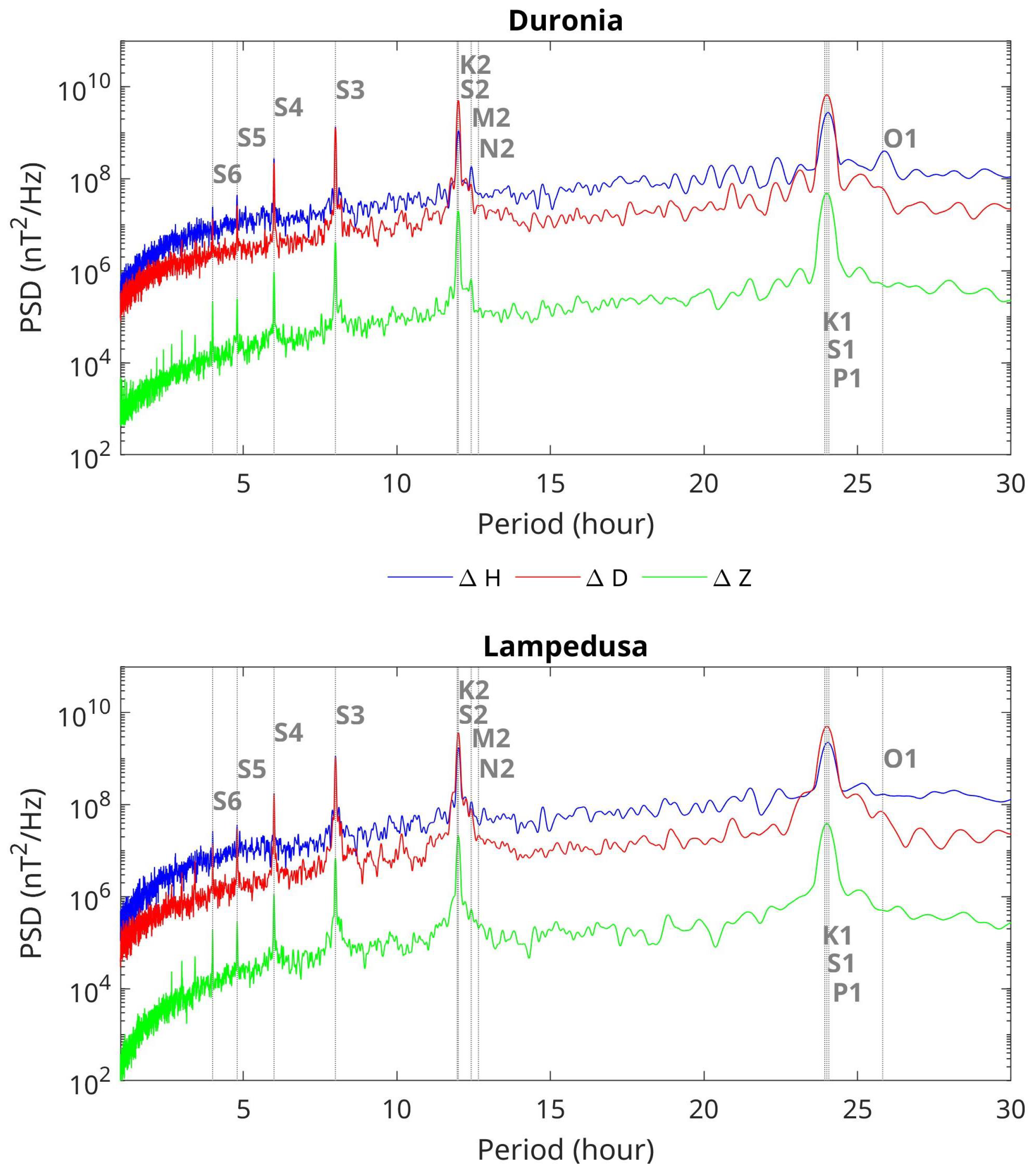
3.1. Geomagnetic Effects of Tidal Modes at Lampedusa and Duronia Observatories

Figure 2 shows the multitaper power spectral density (PSD) estimation of the geomagnetic field components at LMP and DUR, for the years 2017–2018. The tidal mode periods are indicated with vertical bars. The solar high-frequency tidal constituents (S3, …, S6) are well separated and clearly evident in the spectra, while K2 and S2 are not distinguishable because their frequencies are too close, and the same holds also for the K1, S1 and P1 tidal modes. Similar observations come from Larsen [7], for both oceanic and ionospheric media. Conversely, the M2 and O1 tidal modes are well distinguishable in the magnetic signals at both observatories. Moreover, the enhancement corresponding to N2 is weak, detectable only on the D component (red curve), in agreement with the findings of Schnepf et al. [8].

Using nighttime detrended and de-tided geomagnetic data for the years 2017–2020, we applied the robust fitting procedure through the IRLS method to possibly separate the lunar from the solar tidal modes; the de-tiding procedure consists of subtracting the contribution from the tidal modes Sn, n = 1, …, 6, identified through the IRLS method, to the detrended time series obtained through the moving average method described above.

Table 1. Estimated amplitude G and standard errors SE (both expressed in nT) of geomagnetic field variations at tidal mode frequencies obtained through robust fit procedure during nighttime dataset for the years 2017–2020 and for both observatories (Obs.). The lunar tidal modes of interest are marked with the (*) symbol.

			$\mathbf{\Delta }\mathit{H}$		$\mathbf{\Delta }\mathit{D}$		$\mathbf{\Delta }\mathit{Z}$
Tidal Mode	Period (Hours)	Obs.	G	SE	G	SE	G	SE
K2	11.967	LMP	0.450	0.011	0.304	0.007	0.157	0.003
		DUR	0.529	0.011	0.593	0.008	0.171	0.003
M2 *	12.421	LMP	0.514	0.011	0.362	0.007	0.132	0.003
		DUR	0.246	0.011	0.368	0.008	0.210	0.003
N2 *	12.658	LMP	0.184	0.011	0.043	0.007	0.043	0.003
		DUR	0.117	0.011	0.103	0.008	0.074	0.003
K1	23.934	LMP	1.314	0.011	2.058	0.007	0.515	0.003
		DUR	1.676	0.011	2.662	0.008	0.600	0.003
P1	24.066	LMP	1.987	0.011	2.440	0.007	0.775	0.003
		DUR	2.189	0.011	3.136	0.008	0.725	0.003
O1 *	25.819	LMP	0.431	0.011	0.080	0.007	0.125	0.003
		DUR	0.380	0.011	0.140	0.008	0.097	0.003

shows the amplitudes G and their standard errors SE for the geomagnetic tidal modes at the DUR and LMP observatories, selected with p-values < 0.001 and an SE/G ratio < 0.1. The asterisk in brackets (*) refers to the lunar tidal modes of interest. As for previous discussions, the Z component is the relevant indicator of the induction effects. It can be seen from Table 1 that for the tidal modes of interest and for the Z component, larger amplitudes at LMP with respect to DUR are obtained only for the O1 tidal mode.

The gravitational force acts on both the ionosphere and the ocean, leading to superimposed tidal modes at any site. As indicated by Larsen [7], it is possible to evaluate and distinguish the tidal modes contribution from the oceanic and ionospheric source comparing the energy content of the geomagnetic field variations at the M2 and S2 periods, which are very similar (12.421 and 12 h, respectively). Indeed, Larsen [7] concluded that, for coastal and sea floor sites, M2 is mostly driven by the ocean, whereas S2 is mostly driven by the ionosphere. For verifying the relative weight of the two drivers on the S2 and M2 modes, we show their amplitudes in

Table 2. Comparison between S2 (columns 2 and 3) and M2 (columns 4 and 5) tidal modes amplitude for daytime and, in square brackets, nighttime hours at LMP and DUR (values are in nT). Columns 6 and 7: relative day–night differences in M2 tidal amplitude in % (see text for details). The results for the three geomagnetic field components H, D and Z are reported.

	S2 (Day) [S2 (Night)]		M2 (Day) [M2 (Night)]		(M2${}_{\mathit{d}\mathit{a}\mathit{y}}$ − M2${}_{\mathit{n}\mathit{i}\mathit{g}\mathit{h}\mathit{t}}$)/M2${}_{\mathit{d}\mathit{a}\mathit{y}}$
Geomag. Field Component	LMP	DUR	LMP	DUR	LMP	DUR
$\Delta H$	5.1 [0.93]	8.70 [0.69]	0.59 [0.50]	1.72 [0.25]	$+15.4$	$+85.6$
$\Delta D$	8.4 [0.83]	26.30 [0.60]	0.44 [0.37]	1.42 [0.40]	$+16.3$	$+72.2$
$\Delta Z$	2.8 [0.43]	6.30 [0.48]	0.09 [0.15]	0.89 [0.20]	$-75.2$	$+78.0$

, separately for the daytime and nighttime intervals, for DUR and LMP. We note that the S2 amplitude (columns 2 and 3) strongly decreases from day to night at both observatories, as expected for the reduced contribution from the ionospheric electric currents and ionization in the hours of missing solar radiation. For M2, the decrease from daytime to nighttime is very evident at DUR (column 5), while at LMP (column 4), it is very small for the horizontal components H and D. For the Z component, the one more sensitive to inductive processes, there is even an increase during the night, consistently with an oceanic contribution at LMP.

For better investigating the contribution of the ocean and ionosphere, we focus on the M2 tidal mode, computing the day–night relative difference in the M2 amplitude, i.e., (M2${}_{day}$− M2${}_{night}$)/M2${}_{day}$ (%, columns 6 and 7 in Table 2). It can be seen that this relative difference is much larger and positive at DUR than at LMP for all the geomagnetic field components, and the Z component at LMP assumes a negative value. These results confirm that the ionosphere represents the main source of the tidal-related geomagnetic variations for M2 at the inland site of DUR. Conversely, at LMP, the main source of the geomagnetic field variations related to the M2 tidal mode is linked to both the ionospheric (during daytime intervals) and oceanic (during nighttime intervals) drivers.

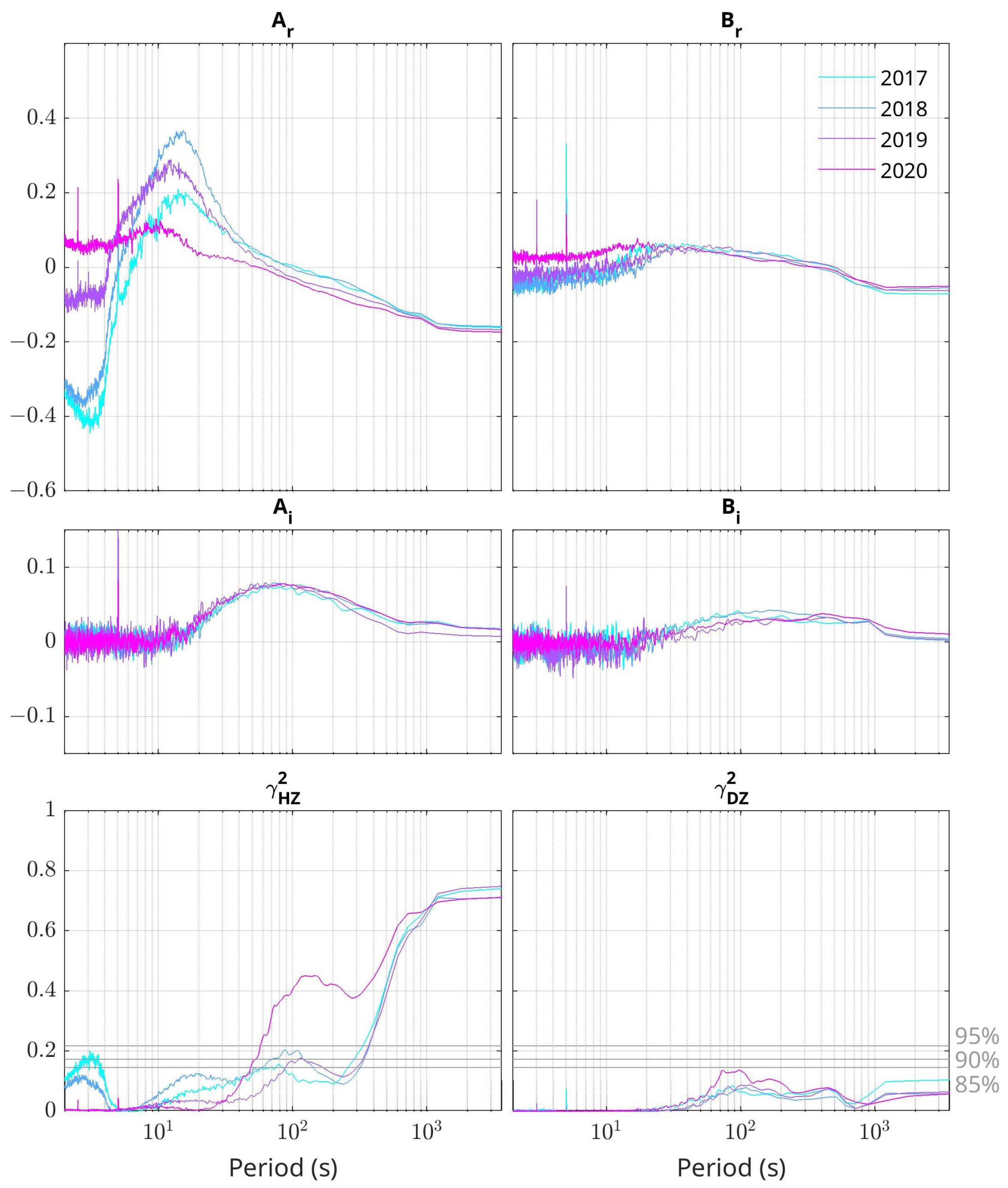
3.2. Transfer Functions and Single-Station Induction Arrows

In this section, we show the relationship between the vertical and horizontal geomagnetic field components at the LMP and DUR observatories. Hereafter, we chose to show the results obtained by comparing the geomagnetic measurements when the data are simultaneously available at both observatories. Differently from what was performed for estimating the signatures of the tidal modes in the magnetic measurements, in this section, we performed the spectral analysis by using 1 h segments after applying a 3 h smoothing procedure. We first investigated the transfer functions and coherence of the geomagnetic field component pairs H-Z and D-Z (${\gamma }_{HZ}^2$ and ${\gamma }_{DZ}^2$, respectively) for the years 2017–2020. For this purpose, for each year, we applied Equation (5), while the representative coherences are computed, accordingly with Equation (7), by using the yearly average spectra and cross-spectra. The significant values can be easily identified by selecting the coherence above a threshold value and then by considering the corresponding $A_r$ and $B_r$. In particular, the coherence thresholds are computed through a Monte Carlo test carried out by using 10,000 couples of 3 h long time series that simulate white noise (e.g., [33,39]). As pointed out by Jones [40], coefficients in Equation (5) have a common dependence on $1/\left(1-{\gamma }_{HD}^2\right)$, suggesting the well-known requirement that H and D must contain some independent information: the horizontal field must not be fully polarized in order to avoid instability in the transfer functions. For this purpose, we selected only time intervals showing a maximum coherence of 0.60 between the horizontal components; this value is sufficiently lower than 1, but it is still high enough to select a significant number of time intervals [19]. In addition, for avoiding ionospheric diurnal effects, we considered only the time interval 18–06 LT.

Figure 3 and Figure 4 show the transfer functions and the coherences at DUR and LMP, respectively, suggesting several features in the two sites. The transfer functions at DUR (maximum amplitude ∼0.7) are generally greater than those at LMP (maximum amplitude ∼0.4). Significant values are obtained at LMP only for the H component and for periods longer than ∼50 s, suggesting that the Z component is mainly related to the H component. At DUR, the transfer functions and coherence attain high values over a wide period range (5 to ∼300 s) for both the H and D components, suggesting that both of them contribute to the Z variations. At LMP, $A_r$ shows a reversal from negative to positive values in the range 4–6 s, a feature particularly evident in the two years 2017–2018. This aspect, however, is not relevant for our purposes because it occurs at the shortest periods, where the coherence is quite low.

We also note contamination at 5 s (and its sub-harmonics) at LMP, corresponding to the sampling rate of the scalar magnetometer. However, this does not represent a problem in our studies because the related monochromatic signals are well distinguishable within the spectra, and they are simply ignored.

In the following pages, we represent the real part of the transfer functions as induction arrows over maps by using the Parkinson convention (i.e., arrows pointing toward areas with a higher electrical conductivity). We show the results for the year 2018 because it is more comprehensive in terms of the data availability at both sites. We decided to show the induction arrows only for the periods corresponding to significant values of the coherence between the vertical and horizontal components: 57–3600 s (∼0.3–18 mHz) at LMP and 5–350 s (∼3–200 mHz) at DUR (Figure 5). For making the SSIAs distinguishable within each map, they are properly rescaled by different factors. It can be seen that at DUR, the majority of the SSIAs point toward the Adriatic coast in the north-east direction, with a rotation toward the north direction for increasing periods up to ∼10 s and then back toward the east for periods up to ∼350 s. Conversely, the coherent group of SSIAs at LMP show a progressive rotation for increasing periods, from the south-west to north-north-east direction.

In order to interpret the peculiar behavior of the SSIAs at LMP, we have to take into account the characteristics of the surrounding region. Assuming that the principal contribution can come from the ocean, and it is related to its bathymetry in the proximity of the island, we retrieved data from EMODnet at 1/16 arc-minute resolution, available at https://www.emodnet-bathymetry.eu/data-products/qaqc-and-dtm-production-details (accessed on 29 November 2022).

Figure 6 shows the location of Lampedusa island and the surrounding bathymetry. By comparing the detailed bathymetry (panel a) with the SSIAs from Figure 5, we can deduce that the SSIAs point toward two deep regions, in the close proximity of the island, around 10 km from the observatory: the SSIAs in the frequency range 2–18 mHz point from north toward the west for an increasing frequency, while the <2 mHz SSIAs point toward the north-north-east.

For better framing the behavior of such observed induction arrows and their dependence on frequency, it is important to understand that the higher conductivity area they point to can be found, besides from the direction given by the direction of the arrow, also from the frequency which gives an indication of its depth. In this regard, the skin depth ${\delta }_{sd}$ of the geomagnetic disturbances propagating horizontally in the sea water is defined by the following equation

$${\delta }_{sd}=\sqrt{\frac{2}{\mu \omega \sigma }}\sim 503.3\sqrt{\rho T},$$

(8)

where $\omega =2\pi f=2\pi /T$ is the angular frequency of the propagating signal (f is the frequency in Hz and $T=1/f$ is the period in s) and $\sigma =1/\rho$ is the conductivity in S/m while $\mu$ represents the magnetic permeability of the sea water which is approximately equal to that of the vacuum ${\mu }_0=4\pi \times {10}^{-7}$ H/m. To evaluate the conductivity representative of the domain of our interest, we applied the Oceanographic Toolbox of Gibbs Seawater [41,42] to the daily ocean data of the Mediterranean sea reanalysis (Simoncelli et al. [43,44]) produced and maintained by the INGV and formerly distributed in the framework of the Copernicus Marine Service (CMEMS). We calculated the annual average conductivity in the surface layer for the period 2017–2018, and we found values in the range of approximately 5.0–5.3 S/m in the surrounding area of the island of Lampedusa. Such results are consistent with those of the World Ocean Data [45] for the same domain.

In principle, the magnetic field variations registered at Lampedusa could be in part due to the signals propagated horizontally from their source located away from the observatory. In the sea, assuming the conductivity range shown above, excluding discontinuities in the conductivity (due to, for example, the presence of an island) and considering the above discussed reliable period (or frequency) range of ∼57–3600 s (∼0.3–18 mHz), we found reasonable values of ${\delta }_{sd}$ in 2–7 km. This means that signals eventually generated in the sea cannot propagate through the sea water to the Lampedusa observatory for distances > 2–7 km because they degrade, becoming uncorrelated with respect to their original nature. These kinds of signals can be regarded as local noises of both an anthropogenic and a natural kind, not contributing significantly to the induction arrows computation. As an example of the degraded (anthropogenic) horizontal signal propagating throughout the subsoil, see Santarelli et al. [46], who examined railway noise at L’Aquila, central Italy.

Regarding the direction of the induction arrows at LMP (Figure 5), we notice different behavior depending on the frequencies, with a direction span much greater than the one we find at DUR. For frequencies of ∼0.3–1.3 mHz, they point to the direction N-NE toward areas of approximately 300 m of bathymetric depth at a distance of ∼10 km, while for higher frequencies, ∼10–18 mHz, they point to the direction W-NW toward bathymetric depths of 100–150 m at a distance of approximately 5–8 km from the observatory.

From the bathymetric map, we can see that a depth of ∼30–50 m represents the typical conditions around Lampedusa island within ∼2–3 km from the observatory. The reason for the observed west direction of the induction arrows at frequencies 5–10 mHz could be attributed to the western location of the observatory with respect to the central part of the island. Conversely, the observatory is almost central with respect to the south-north extension of the island, and the higher conductive region, corresponding to the greater ocean depth, is located in the N-NE direction pointed by induction arrows in the frequencies < 1.3 mHz.

In the Sicily channel, there are two main seawater streams (the Atlantic Tunisian Current and Atlantic Ionian Stream, see Jouini et al. [47]) having a direction from NW to SE which can give a static magnetic signature, associated to the average flow intensity, and a transient one associated to its variations. These magnetic signatures are not persistent at the frequencies we analyze; therefore, they are not taken into account in the present work. Moreover, the distance of the LMP observatory from the regions where these seawater streams flow is largely greater than the limit of ∼10 km associated to the skin depth of the signals which propagate in the horizontal direction (the white circles in Figure 6 indicate points 10 and 20 km distance from LMP).

We also note that the amplitude of the induction arrows is greater at DUR than at LMP. This feature can be well explained in terms of a coast effect at DUR (indeed, the arrows’ direction is within a cone toward the Adriatic sea), while at LMP, a small island, the coast effect from the surrounding sea mostly compensates, with a residual toward the west due to the non-central position of the observatory on the island, and the predominant effect is in the N-NE and W-NW directions due to the greater depth sea regions.

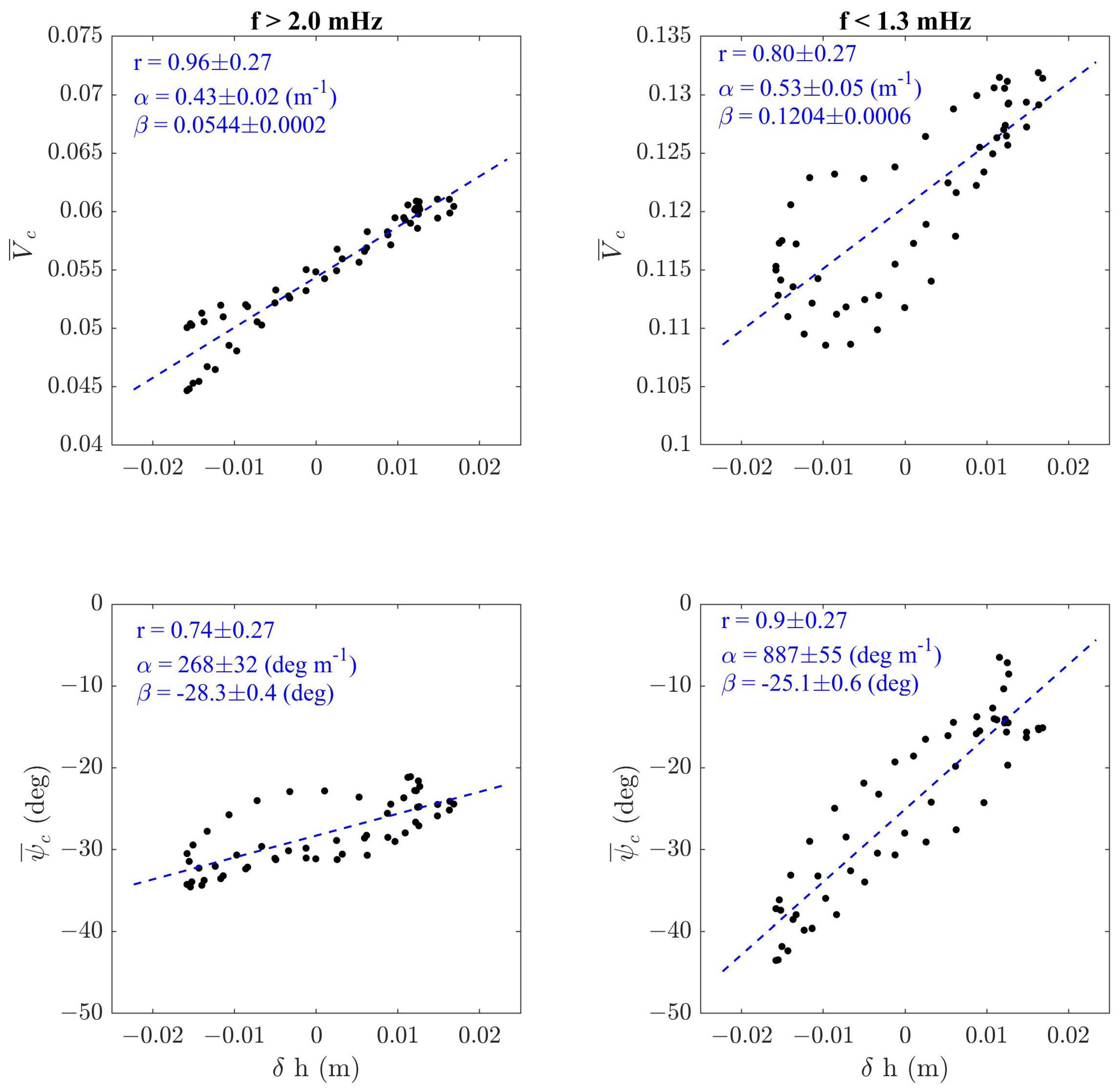
3.3. Dependency of Transfer Functions on the Lunar O1 Tidal Mode Sea Level Change

In Section 3.1, we showed evidence of the correlation between the sea level variations and the geomagnetic field variations. In Section 3.2, we also showed that reliable induction effects at different time scales are probably related to ocean regions characterized by different depths. We are now interested in investigating the possible effects of a sea level change at periods reported in Table 1 on the induction arrows. To study the dependency of the induction arrows on the tidal modes, we applied the Superposed Epoch Analysis (SEA) technique on the amplitude and phase of the SSIAs for LMP and, for comparison, the DUR geomagnetic data. The analysis was based on the O1 constituent, albeit it is not as energetic as other lunar components, such as N2 or M2. However, its period (approximately 25.83 h) is sufficiently far from the diurnal and semidiurnal periods (24 and 12 h) to prevent the occurrence of peaks at approximately the same time throughout the day. This allows the distribution of the O1-induced peaks in different local times, thus making sure we avoid possible local time effects triggered by ionospheric/magnetospheric currents. The barotropic tidal analysis was based on the observed data from the National Italian Mareographic Network (RMN–Rete Mareografica Nazionale, https://www.mareografico.it/ (accessed on 29 November 2022)) managed by the ISPRA (https://www.isprambiente.gov.it (accessed on 29 November 2022)). The raw data acquired have a sampling rate of 10 min. Before using them for our analysis, they were thoroughly quality checked and cleaned in terms of spikes, instrument tilting and persisted or missing records and smoothed through a one-hour rolling window average centered on the single observation.

In the SEA approach, we need to superimpose an ensemble of stochastically independent time series, possibly containing significant signals, of the same length. We call zero epochs the instants of maximum barotropic height $\delta h_{max}$; this is the central time of the time series for which we require a length of ±48 h to adequately include a previous and a following peak. The procedure adopted for selecting the lunar tidal events is described as follows. The barotropic level $\delta h$ is band-pass filtered at periods of 25–27 h for isolating the O1 tidal mode; the minimum $\delta h_{min}$ = 0.01 m and a minimum separation of 48 h between peaks chosen as the zero epoch is imposed. This latter criterion is requested to guarantee a stochastic independence between the time series for computing the composite means.

For realizing a time series of the amplitude and phase of the SSIAs consistently with each selected time series of barotropic level $\delta h$, the following steps should be satisfied:

• The geomagnetic field variations around the selected ith-epoch and for a time interval ±48 h are linearly detrended;
• The selected geomagnetic time series are Fourier analyzed by considering a 1/2 h moving time series (so the time resolution of dynamic spectra is 1/2 h) of a duration of 3 h spanning the ±48 h time interval. For each moving subset, we computed the auto-spectra and cross-spectra following Welch’s method, i.e., subdividing the 3 h time window into the 1 h time window with a 67% overlap;
• Around each time $\tau$ with respect to the zero epoch ($\tau$ = 0), the transfer function coefficients are computed both in the amplitude and phase following Equations (4) and (5) by using 20 spectra and cross-spectra. This number of chosen spectra allows to reach reliable SSIA amplitudes and phases (in the least squares sense) and short time uncertainties.

This procedure led to the creation of 229 independent time series, which are the composite O1 signals.

The time-varying transfer function coefficients constructed as described above represent the time-varying composite transfer functions. Finally, they are averaged in the SEA procedure, providing the composite mean time-varying transfer function referred to as $V_c$ and ${\psi }_c$ (where “c” indicates the composite mean) and the respective standard error of the mean (SEM). The above described methodology was applied for the years 2017–2020, and the results are shown in Figure 7. The composite mean of the barotropic sea level is the solid thick black line of panel a of Figure 7, and it was computed by averaging 229 selected time intervals. The error bars, of amplitude 1.96 SEM, correspond to a confidence bound of 95%. The red lines indicate the 95% confidence bound obtained through a Monte Carlo test run 10,000 times on 229 white noise surrogates randomly generated, each with a standard deviation and mean equal to that of a corresponding composite of a filtered O1 tidal signal (see [48] for the method and [49] for an application).

A clear correspondence between the transfer function amplitude and phase and the sea level variations can be identified at the LMP observatory (panels b and c). In detail, we note that this correspondence is very clear for the frequencies > 2 mHz as well as for the lowest frequencies, while around 2 mHz, the correspondence disappears. Conversely, no correlations are observed at DUR for any frequency range (panels d and e).

The correlation between the mean composite transfer functions (both the amplitude $V_c$ and phase ${\psi }_c$) and the sea level ($\delta h$) was also assessed from a quantitative point of view for the O1 constituent at LMP. We first computed the averages of $V_c$ and ${\psi }_c$ in the two frequency ranges where the correlation is more significant, that is, f > 2.0 mHz and f < 1.3 mHz, hereafter referred to as ${\overline{V}}_c$ and ${\overline{\psi }}_c$. Then, we computed the cross-correlation between these two quantities (for f > 2.0 and f < 1.3 mHz) and the barotropic sea level fluctuations $\delta h$ at the O1 tidal mode derived from the SEA.

The correlation coefficients r and the results of the linear regression between $\delta h$ and both ${\overline{V}}_c$ and ${\overline{\psi }}_c$ ($\propto \alpha \delta h+\beta$) are reported in Figure 8. The $\alpha$ values show that an amplitude increase of $\delta {\overline{V}}_c\sim 4\times {10}^{-3}$ ($\sim 5\times {10}^{-3}$) and an azimuthal increment of $\delta {\overline{\psi }}_c\sim 3^{\circ }$ ($\sim 9^{\circ }$) are expected for $\delta h$ = 1 cm for f > 2 mHz (<1.3 mHz).

4. Discussion

Tidal modes, induced by the Sun–Earth–Moon gravitational system, generate ionospheric as well as oceanic induced current systems [7]. We verified the presence of geomagnetic signatures in dataset from two geomagnetic Italian observatories, one located on a small island, LMP, the other one inland, DUR. As shown in Figure 2, evidence of solar and lunar tidal modes is found in each component of the Earth’s magnetic field recorded at both observatories. All solar tidal constituents of periods up to 8 h (S6, …, S3) are well distinguishable, while the S2 and S1 constituents are not resolved with respect to K2 and K1, and P1, respectively, because the periods are very close. We are interested in the oceanic effects, so we do not focus on the Sn components, whose geomagnetic signature is mainly linked to ionospheric effects, but rather on the other two evident components, M2 and O1, lunar semidiurnal and diurnal, respectively, disregarding the weak, hardly detectable N2 component [8].

For distinguishing the oceanic and ionospheric contribution to tidal modes, we focused on the M2 and S2 modes, whose periods are quite close (12.421 and 12 h, respectively), following the assumption that, according to [7], S2 is mostly driven by the ionosphere while M2, at coastal sites, is mostly driven by the ocean. In particular, we compared their amplitudes for the daytime and nighttime hours. We verified that for the inland observatory, the M2 amplitude is much greater during the day when the ionospheric contribution is also active. Conversely, for the island observatory, the M2 amplitude does not change significantly between the day and night, because the main contribution comes from the ocean. A further confirmation that geomagnetic field variations corresponding to the lunar semidiurnal M2 mode are due to ionospheric (at daytime) and oceanic (at nighttime) drivers at LMP was given by the low values of the day–night amplitude relative difference. On the contrary, these variations are mainly due to the ionospheric drivers at DUR, regardless of the local time, as indicated by the higher values of the day–night amplitude relative difference.

Another tool for characterizing the different behavior of the influence of the ocean in the geomagnetic field at LMP and DUR is the computation of transfer functions, dependent on frequency, represented as single-station induction arrows (SSIAs) over maps. Figure 5 shows such SSIAs only for the frequencies corresponding to significant values of the coherence between the vertical and horizontal geomagnetic field components. Induction arrows are used to recognize the properties of the surrounding environment, because they point toward the areas with a higher electrical conductivity. Different frequencies correspond to different skin depths, decreasing for an increasing frequency. In this context, we find that at DUR, the majority of the SSIAs point toward the Adriatic coast in the north-east direction. This suggests a coast effect at DUR similar to that found for inland stations in Italy [17] and in Croatia [18], in both cases for periods longer than 10 min. In particular, Armadillo et al. [17] found, in central Italy, a clear double regime, the Adriatic and the Tyrrhenian domain which are separated by the Apennine chain running in the middle. After a wide consideration of a seismic, heat flow, resistivity and geomagnetic dataset for the area under study which is rather complex, 2D model responses showed that a deep conductive layer (>5000 S) underlies the Apennine chain at about a 20 km depth (interpreted as a sort of root of the chain) and the transition between the Adriatic and the Tyrrhenian regimes is marked by a rather sharp vertical offset in this conducting layer. This determines the behavior of the induction arrows observed in the two domains, and Duronia, belonging to the Adriatic domain, is mainly influenced by the Adriatic sea.

For LMP, we find that the lower frequency induction arrows point toward the N-NE direction where, at a distance of ∼10 km, the ocean bathymetric depth steeply reaches approximately 300 m. Conversely, for higher frequencies, the SSIAs point to the W-NW direction where, at a distance of ∼5–8 km, the ocean bathymetric depth reaches approximately 100–150 m.

For small islands, such as Lampedusa, the coast effect is less clear, because the contribution from the surrounding sea mostly compensates; moreover, previous works showed a different behavior at small islands with respect to inland sites (e.g., [7,8,20,21]). In our case, at LMP, in the N-S direction, the coast effect compensates, and the predominant effect is due to the already discussed sea regions at a greater depth. Conversely, a residual coast effect toward the west due to the non-central position of the observatory on the island in the E-W direction is detected. On the other hand, in the N-S direction, the predominant effect is due to the deeper sea regions. These results reflect several typical aspects of geomagnetic observatories located on small islands like Lampedusa (e.g., [7,8,20]).

Then, we investigated the magnetic signature of the sea level changes due to the tidal modes to quantify the effect of the sea level change on the geomagnetic data. For accomplishing this task, we focused on the O1 mode, which has a lower energetic content with respect to N2 or M2, but whose period (approximately 25.83 h, sufficiently far from 24 and 12 h) allows to obtain independent information not contaminated by the well-known diurnal and semidiurnal geomagnetic effects triggered by ionospheric/magnetospheric currents. We applied a statistical SEA approach over a 4-year interval (2017 to 2020) of the amplitude and phase of the induction arrows from a dataset of both geomagnetic observatories and the corresponding sea level barotropic heights. Figure 7 suggests some important outcomes. In the data of the DUR observatory, located far from the sea where the ULF waves are not influenced by small sea level changes, we do not find any significant pattern of geomagnetic parameters related to the O1 frequency, at no frequencies of the geomagnetic field. On the contrary, the geomagnetic field measurements at the LMP observatory, which are affected by the presence of the close, surrounding sea, show a clear correlation between the transfer function amplitude and phase and the sea level variations induced by the O1 tide constituent at frequencies higher than 2.0 mHz and lower than 1.3 mHz. In between, around 2.0 mHz, the geomagnetic parameters are quite constant, suggesting a passage between the two regimes. Finally, we quantified the contribution of the sea level variations $\delta h$ due to the O1 tidal mode to the geomagnetic transfer functions at LMP, averaged over the two frequency ranges where the correlation is more significant, that is, f > 2.0 mHz and f < 1.3 mHz (amplitude ${\overline{V}}_c$ and phase ${\overline{\psi }}_c$). Through a linear regression, we found that an increment of the sea level $\delta h$ = 1 cm corresponds to an amplitude increase of $\delta {\overline{V}}_c\sim 4\times {10}^{-3}$ (∼$5\times {10}^{-3}$) and to a phase increase of $\delta {\overline{\psi }}_c\sim 3^{\circ }$ (∼$9^{\circ }$) for f > 2 mHz (<1.3 mHz).

5. Conclusions

We investigated the tidal effect in the geomagnetic field components at the Lampedusa and, for comparison, Duronia geomagnetic observatories during the years 2017–2020. The main results of the study can be summarized as follows:

1.

The tidal modes of the internal (oceanic) and external (ionospheric) sources are found at both sites and for both the solar and lunar gravitational forces, in agreement with past investigations.

2.

Through a robust fit analysis of the geomagnetic field variations, and through a comparison between the nighttime and daytime data, it was evidenced that on the geomagnetic signature of the M2 barotropic tidal mode, the oceanic contribution is dominant at Lampedusa with respect to the ionospheric contribution, in agreement with other investigations on similar sites. On the contrary, at Duronia, which is an inland site, the ionospheric contribution is dominant both at daytime and nighttime.

3.

The geomagnetic field variations investigated in the spectral domain through transfer functions clearly indicated a different response along the Z component at the two sites, which is reflected in the different behavior of the induction vectors. At DUR, a coast effect emerges, with arrows directed toward the Adriatic sea. At LMP, which is a small island, the coast effect is partially canceled due to the island geometry, with a residual toward the west due to the westernmost position of the observatory, and with the highest amplitude arrows pointing toward the surrounding regions with a higher conductivity in correspondence to a deeper ocean.

4.

Through the Superposed Epoch Analysis applied to the O1 tidal mode, we found that the induction arrows at LMP are strongly correlated to sea level variations. Indeed, in correspondence to a sea level change of 1 cm, the transfer functions for frequencies f > 2 mHz (<1.3 mHz) show an increase of ∼$4\times {10}^{-3}$ (∼$5\times {10}^{-3}$) in the amplitude and ∼$3^{\circ }$ (∼$9^{\circ }$) in the phase.

This last result, i.e., the establishment of a correlation between the sea level changes and the transfer function from horizontal to vertical geomagnetic field components, in the ULF range, could provide new and original diagnostic tools based on magnetic field measurements, remarking on the importance of island sites such as Lampedusa.

References

1. van Bemmelen, W. Die lunare Variation des Erdmagnetismus. Meteorol. Z. 1912, 29, 218–225. [Google Scholar]
2. van Bemmelen, W. Berichtigung zu meiner Abhandlung über die lunare Variation des Erdmagnetismus. Meteorol. Z. 1913, 30, 589–594. [Google Scholar]
3. Chapman, S.I. The solar and lunar diurnal variations of terrestrial magnetism. Philos. Trans. R. Soc. Lond. Ser. A Contain. Pap. Math. Phys. Character 1919, 218, 1–118. [Google Scholar] [CrossRef]
4. Chapman, S.; Bartels, J. Geomagnetism, Vol. I and II; Oxford University Press: Oxford, UK, 1940. [Google Scholar]
5. Matsushita, S.; Maeda, H. On the geomagnetic solar quiet daily variation field during the IGY. J. Geophys. Res. 1965, 70, 2535–2558. [Google Scholar] [CrossRef]
6. Egedal, J. The lunar-diurnal magnetic variation and its relation to the solar-diurnal variation. J. Geophys. Res. 1956, 61, 748–749. [Google Scholar] [CrossRef]
7. Larsen, J.C. Electric and Magnetic Fields Induced by Deep Sea Tides. Geophys. J. Int. 1968, 16, 47–70. [Google Scholar] [CrossRef] [Green Version]
8. Schnepf, N.R.; Manoj, C.; Kuvshinov, A.; Toh, H.; Maus, S. Tidal signals in ocean-bottom magnetic measurements of the Northwestern Pacific: Observation versus prediction. Geophys. J. Int. 2014, 198, 1096–1110. [Google Scholar] [CrossRef] [Green Version]
9. Richmond, A. Modeling equatorial ionospheric electric fields. J. Atmos. Terr. Phys. 1995, 57, 1103–1115. [Google Scholar] [CrossRef]
10. Kelley, M.C. The Earth’s Ionosphere, Plasma Physics and Electrodynamics, 2nd ed.; Academic Press, Inc.: San Diego, CA, USA, 1989; ISBN 9780120884254. [Google Scholar]
11. Simpson, F.; Bahr, K. Practical Magnetotellurics; Cambridge University Press: Cambridge, UK, 2005; ISBN 9780511614095. [Google Scholar] [CrossRef]
12. Berdichevsky, M.N.; Dmitriev, V.I. Models and Methods of Magnetotellurics; Springer: Berlin, Germany, 2008. [Google Scholar] [CrossRef]
13. Parkinson, W.D. The Influence of Continents and Oceans on Geomagnetic Variations. Geophys. J. Int. 1962, 6, 441–449. [Google Scholar] [CrossRef] [Green Version]
14. Parkinson, W.D. Directions of Rapid Geomagnetic Fluctuations. Geophys. J. Int. 1959, 2, 1–14. [Google Scholar] [CrossRef]
15. Parkinson, W.D.; Jones, F.W. The geomagnetic coast effect. Rev. Geophys. 1979, 17, 1999. [Google Scholar] [CrossRef]
16. Hitchman, A.P.; Milligan, P.R.; Lilley, F.T.; White, A.; Heinson, G.S. The total-field geomagnetic coast effect: The CICADA97 line from deep Tasman Sea to inland New South Wales. Explor. Geophys. 2000, 31, 52–57. [Google Scholar] [CrossRef] [Green Version]
17. Armadillo, E.; Bozzo, E.; Cerv, V.; Santis, A.D.; Mauro, D.D.; Gambetta, M.; Meloni, A.; Pek, J.; Speranza, F. Geomagnetic depth sounding in the Northern Apennines (Italy). Earth Planets Space 2001, 53, 385–396. [Google Scholar] [CrossRef] [Green Version]
18. Vujić, E.; Brkić, M. Geomagnetic coast effect at two Croatian repeat stations. Ann. Geophys. 2017, 59, G0652. [Google Scholar]
19. Regi, M.; De Lauretis, M.; Francia, P.; Lepidi, S.; Piancatelli, A.; Urbini, S. The geomagnetic coast effect at two 80°S stations in Antarctica, observed in the ULF range. Ann. Geophys. 2018, 36, 193–203. [Google Scholar] [CrossRef] [Green Version]
20. Samrock, F.; Kuvshinov, A. Tippers at island observatories: Can we use them to probe electrical conductivity of the Earth’s crust and upper mantle? Geophys. Res. Lett. 2013, 40, 824–828. [Google Scholar] [CrossRef]
21. Morschhauser, A.; Grayver, A.; Kuvshinov, A.; Samrock, F.; Matzka, J. Tippers at island geomagnetic observatories constrain electrical conductivity of oceanic lithosphere and upper mantle. Earth Planets Space 2019, 71. [Google Scholar] [CrossRef] [Green Version]
22. Di Mauro, D.; Regi, M.; Lepidi, S.; Del Corpo, A.; Dominici, G.; Bagiacchi, P.; Benedetti, G.; Cafarella, L. Geomagnetic Activity at Lampedusa Island: Characterization and Comparison with the Other Italian Observatories, Also in Response to Space Weather Events. Remote Sens. 2021, 13, 3111. [Google Scholar] [CrossRef]
23. Amante, C.; Eakins, B.W. ETOPO1 1 Arc-Minute Global Relief Model: Procedures, Data Sources and Analysis. NOAA Technical Memorandum NESDIS NGDC-24. 2009. Available online: https://repository.library.noaa.gov/view/noaa/1163. https://www.ngdc.noaa.gov/mgg/global/relief/ETOPO1/docs/ETOPO1.pdf (accessed on 29 November 2022). [CrossRef]
24. Pawlowicz, R. M_Map: A Mapping Package for MATLAB. 2020. Available online: http://www.eoas.ubc.ca/~rich/map.html (accessed on 29 November 2022).
25. Civile, D.; Lodolo, E.; Tortorici, L.; Lanzafame, G.; Brancolini, G. Relationships between magmatism and tectonics in a continental rift: The Pantelleria Island region (Sicily Channel, Italy). Mar. Geol. 2008, 251, 32–46. [Google Scholar] [CrossRef]
26. Civile, D.; Lodolo, E.; Alp, H.; Ben-Avraham, Z.; Cova, A.; Baradello, L.; Accettella, D.; Burca, M.; Centonze, J. Seismic stratigraphy and structural setting of the Adventure Plateau (Sicily Channel). Mar. Geophys. Res. 2013, 35, 37–53. [Google Scholar] [CrossRef]
27. Regi, M.; Corpo, A.D.; De Lauretis, M. The use of the empirical mode decomposition for the identification of mean field aligned reference frames. Ann. Geophys. 2017, 59. [Google Scholar] [CrossRef]
28. Thomson, D. Spectrum estimation and harmonic analysis. Proc. IEEE 1982, 70, 1055–1096. [Google Scholar] [CrossRef] [Green Version]
29. Huber, P.J. Robust Statistics; Wiley Series in Probability and Statistics; Wiley: New York, NY, USA, 1981. [Google Scholar] [CrossRef]
30. De Lauretis, M.; Francia, P.; Regi, M.; Villante, U.; Piancatelli, A. Pc3 pulsations in the polar cap and at low latitude. J. Geophys. Res. Space Phys. 2010, 115, A11223. [Google Scholar] [CrossRef] [Green Version]
31. Everett, J.; Hyndman, R. Geomagnetic variations and electrical conductivity structure in south-western Australia. Phys. Earth Planet. Inter. 1967, 1, 24–34. [Google Scholar] [CrossRef]
32. Francia, P.; Regi, M.; Lauretis, M.D.; Villante, U.; Pilipenko, V.A. A case study of upstream wave transmission to the ground at polar and low latitudes. J. Geophys. Res. Space Phys. 2012, 117. [Google Scholar] [CrossRef]
33. Regi, M.; Francia, P.; De Lauretis, M.; Glassmeier, K.H.; Villante, U. Coherent transmission of upstream waves to polar latitudes through magnetotail lobes. J. Geophys. Res. Space Phys. 2013, 118, 6955–6963. [Google Scholar] [CrossRef]
34. Regi, M.; De Lauretis, M.; Francia, P.; Villante, U. The propagation of ULF waves from the Earth’s foreshock region to ground: The case study of 15 February 2009. Earth Planets Space 2014, 66, 1–9. [Google Scholar] [CrossRef] [Green Version]
35. Regi, M.; De Lauretis, M.; Francia, P. The occurrence of upstream waves in relation with the solar wind parameters: A statistical approach to estimate the size of the foreshock region. Planet. Space Sci. 2014, 90, 100–105. [Google Scholar] [CrossRef]
36. Schmucker, U. Anomalies of Geomagnetic Variations in the Southwestern United States; Number 13 in Bull. Scripps Inst. Oceanography Univ. California; University of California Press: Berkeley, CA, USA, 1970; pp. 127–132. [Google Scholar]
37. Wiese, H. Geomagnetische Tiefentellurik Teil II: Die Streichrichtung der untergrundstrukturen des elektrischen Widerstandes, erschlossen aus geomagnetischen Variationen. Geofis. Pura Appl. 1962, 52, 83–103. [Google Scholar] [CrossRef]
38. Bendat, J.S.; Piersol, A.G. Random Data. Analysis and Measurement Procedures, 1st ed.; John Wiley & Sons: Hoboken, NY, USA, 1971. [Google Scholar]
39. Regi, M.; De Lauretis, M.; Redaelli, G.; Francia, P. ULF geomagnetic and polar cap potential signatures in the temperature and zonal wind reanalysis data in Antarctica. J. Geophys. Res. Space Phys. 2016, 121, 286–295. [Google Scholar] [CrossRef]
40. Jones, A. Geomagnetic Induction Studies in Scandinavia. II. Geomagnetic Depth Sounding, Induction Vectors and Coast-Effect. J. Geophys. 1981, 50, 23–36. [Google Scholar]
41. McDougal, T.J.; Barker, P.M. Getting started with TEOS-10 and the Gibbs Seawater (GSW) Oceanographic Toolbox; Trevor J. McDougall. 2011. Available online: http://www.teos-10.org/software.htm (accessed on 29 November 2022).
42. IOC; SOR; IAPSO. The international thermodynamic equations of seawater-2010: Calculation and use of thermodynamic properties. Intergov. Oceanogr. Comm. Manuals Guid. 2010, 56, 196. [Google Scholar]
43. Simoncelli, S.; Masina, S.; Axell, L.; Liu, Y.; Salon, S.; Cossarini, G. MyOcean Regional Reanalyses: Overview of Reanalyses Systems and Main Results. Mercat. Ocean J. 2016, 54, 116. Available online: https://www.mercator-ocean.eu/wp-content/uploads/2016/03/JournalMO-54.pdf (accessed on 29 November 2022).
44. Simoncelli, S.; Fratianni, C.; Pinardi, N.; Grandi, A.; Drudi, M.; Oddo, P.; Srdjan, D. Mediterranean Sea physical reanalysis (MEDREA). Copernic. Monit. Environ. Mar. Serv. (CMEMS) 2019. [Google Scholar] [CrossRef]
45. Tyler, R.H.; Boyer, T.P.; Minami, T.; Zweng, M.M.; Reagan, J.R. Electrical conductivity of the global ocean. Earth Planets Space 2017, 69, 1–10. [Google Scholar] [CrossRef] [Green Version]
46. Santarelli, L.; Palangio, P.; Lauretis, M.D. Electromagnetic background noise at L’Aquila Geomagnetic Observatory. Ann. Geophys. 2014, 57, G0211. [Google Scholar] [CrossRef]
47. Jouini, M.; Béranger, K.; Arsouze, T.; Beuvier, J.; Thiria, S.; Crépon, M.; Taupier-Letage, I. The Sicily Channel surface circulation revisited using a neural clustering analysis of a high-resolution simulation. J. Geophys. Res. Ocean. 2016, 121, 4545–4567. [Google Scholar] [CrossRef] [Green Version]
48. Laken, B.A.; Čalogović, J. Composite analysis with Monte Carlo methods: An example with cosmic rays and clouds. J. Space Weather. Space Clim. 2013, 3, A29:1–A29:13. [Google Scholar] [CrossRef]
49. Regi, M.; Redaelli, G.; Francia, P.; De Lauretis, M. ULF geomagnetic activity effects on tropospheric temperature, specific humidity, and cloud cover in Antarctica, during 2003–2010. J. Geophys. Res. Atmos. 2017, 122, 6488–6501. [Google Scholar] [CrossRef]
Figure 1. The location of two Italian geomagnetic observatories of LMP and DUR (red filled circles) used in this work together with their geographic coordinates. Map produced by M_Map software [24].
Remotesensing 14 06203 g001
Figure 2. Multitaper power spectral densities for the Δ H (blue), Δ D (red) and Δ Z (green) at DUR (top) and LMP (bottom) by using multitaper method for the years 2017–2018. Tidal mode periods are indicated with vertical gray dotted lines. In both panels, Δ H and Δ D spectra are multiplied by a factor 40 and 20, respectively, to make curves distinguishable from each other.
Remotesensing 14 06203 g002
Figure 3. Transfer functions at DUR for the pairs HZ (left) and DZ (right) in both real (r) and imaginary (i) parts. Bottom panels report the ordinary (univariate) coherences between vertical and horizontal components. In the bottom panels, the coherence thresholds at 85, 90 and 95%, estimated by a Monte Carlo method, are shown as horizontal gray lines.
Remotesensing 14 06203 g003
Figure 4. Transfer functions at LMP for the pairs HZ (left) and DZ (right) in both real (r) and imaginary (i) parts. Bottom panels report the ordinary (univariate) coherences between vertical and horizontal components. In the bottom panels, the coherence thresholds at 85, 90 and 95%, estimated by a Monte Carlo method, are shown as horizontal gray lines.
Remotesensing 14 06203 g004
Figure 5. Single-station induction arrows, for real V ( r ) , at LMP (top panel) and DUR (bottom panel) in 2018 and in the reliable frequency/period range (see text for details). The origin of induction arrows corresponds to the observatory position. The frequencies are indicated by colorbars, while the reference amplitude of 0.1 and 0.2 length for the arrows are shown as segments along both longitude and latitude. Map produced by M_Map software [24].
Remotesensing 14 06203 g005
Figure 6. Bathymetry maps (color scales) of the (b) Mediterranean region of our interest and (a) detail around Lampedusa island. The latter region is also marked as green square in panel (b). White dashed circles, both centered at LMP observatory, indicate 10 and 20 km distant points. Different color scales are used for a better recognition of regional bathymetry. Map produced by M_Map software [24].
Remotesensing 14 06203 g006
Figure 7. SEA results of SSIA at DUR and LMP. Panel (a): superposition of 229 tidal events (gray lines) during 2017–2020 at periods of ∼26 h and their composite mean (black line). Panels (b,c): composite means of log-scale amplitude V c and phase ψ c at LMP. Panels (d,e): same as panels (b,c) but for DUR. The horizontal blue bar in panel (c) indicates the time uncertainty δ T ∼3 h functional to the spectral analysis (see text for details). The vertical dashed gray lines mark the uncertainty in determining τ (i.e., τ ± Δ τ ) in correspondence of maximum δ h of each composite.
Remotesensing 14 06203 g007
Figure 8. Cross-correlation between averaged composites mean amplitude V ¯ c (top panels) and phase ψ ¯ c (bottom panels) of transfer functions at LMP for f > 2.0 (left panels) and f < 1.3 mHz (right panels) and barotropic sea level fluctuations δ h at O1 tidal mode derived from SEA (see text for details). α and β coefficients of linear fit are shown together with the correlation coefficient r and their 95% threshold estimated by null-hypothesis with 55 degrees of freedom.
Remotesensing 14 06203 g008