
Modeling Shadow with Voxel-Based Trees for Sentinel-2 Reflectance Simulation in Tropical Rainforest


Abstract
:1. Introduction
2. Methodology
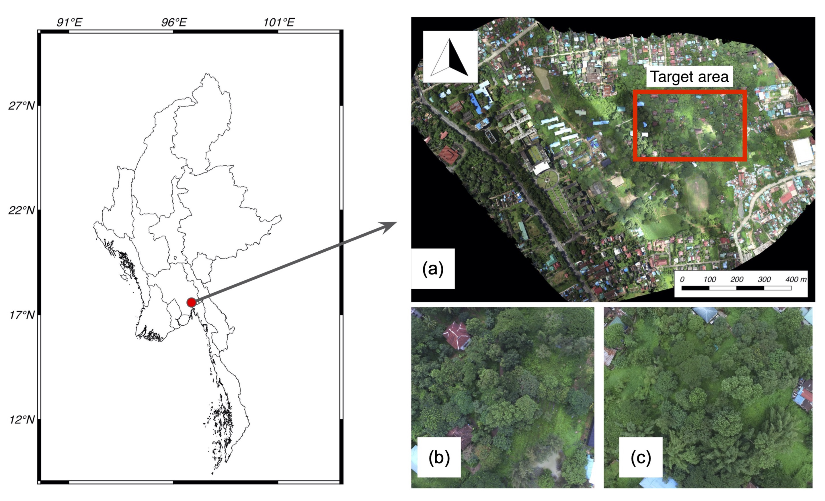
2.1. Study Area
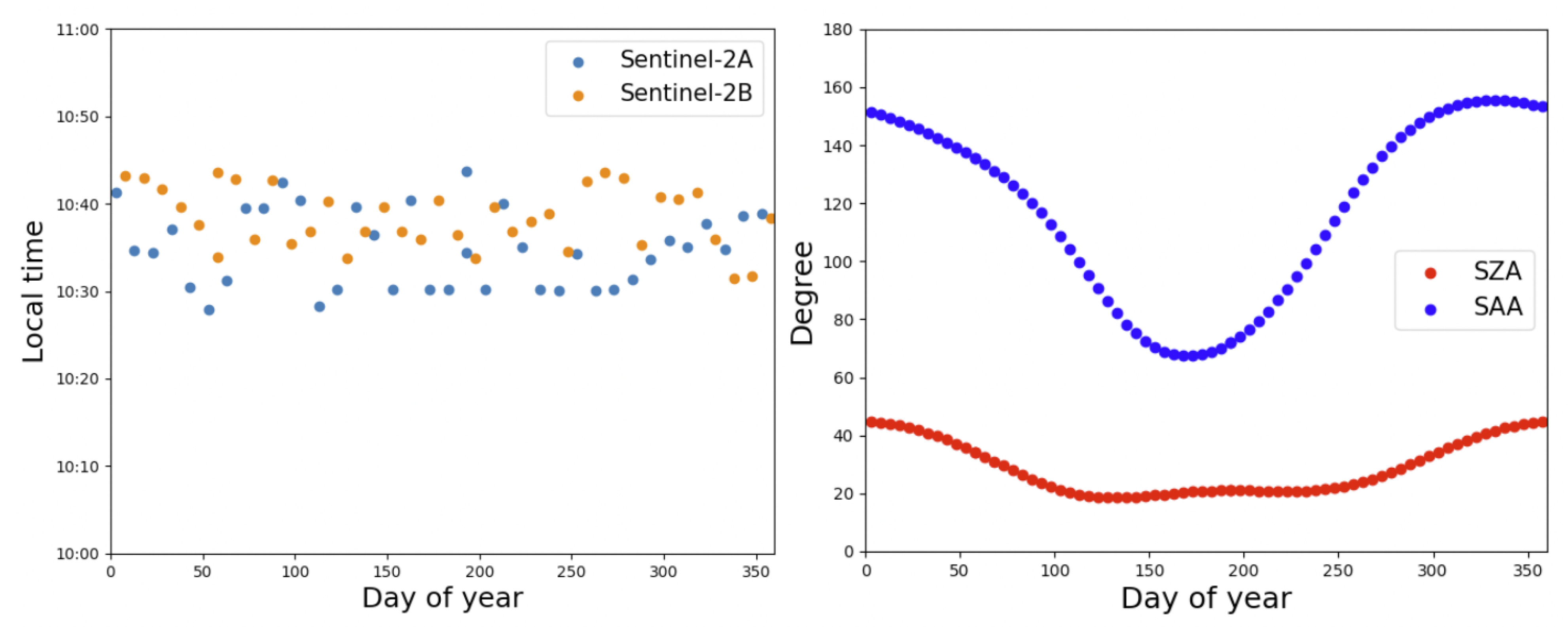
2.2. Sentinel-2 Image
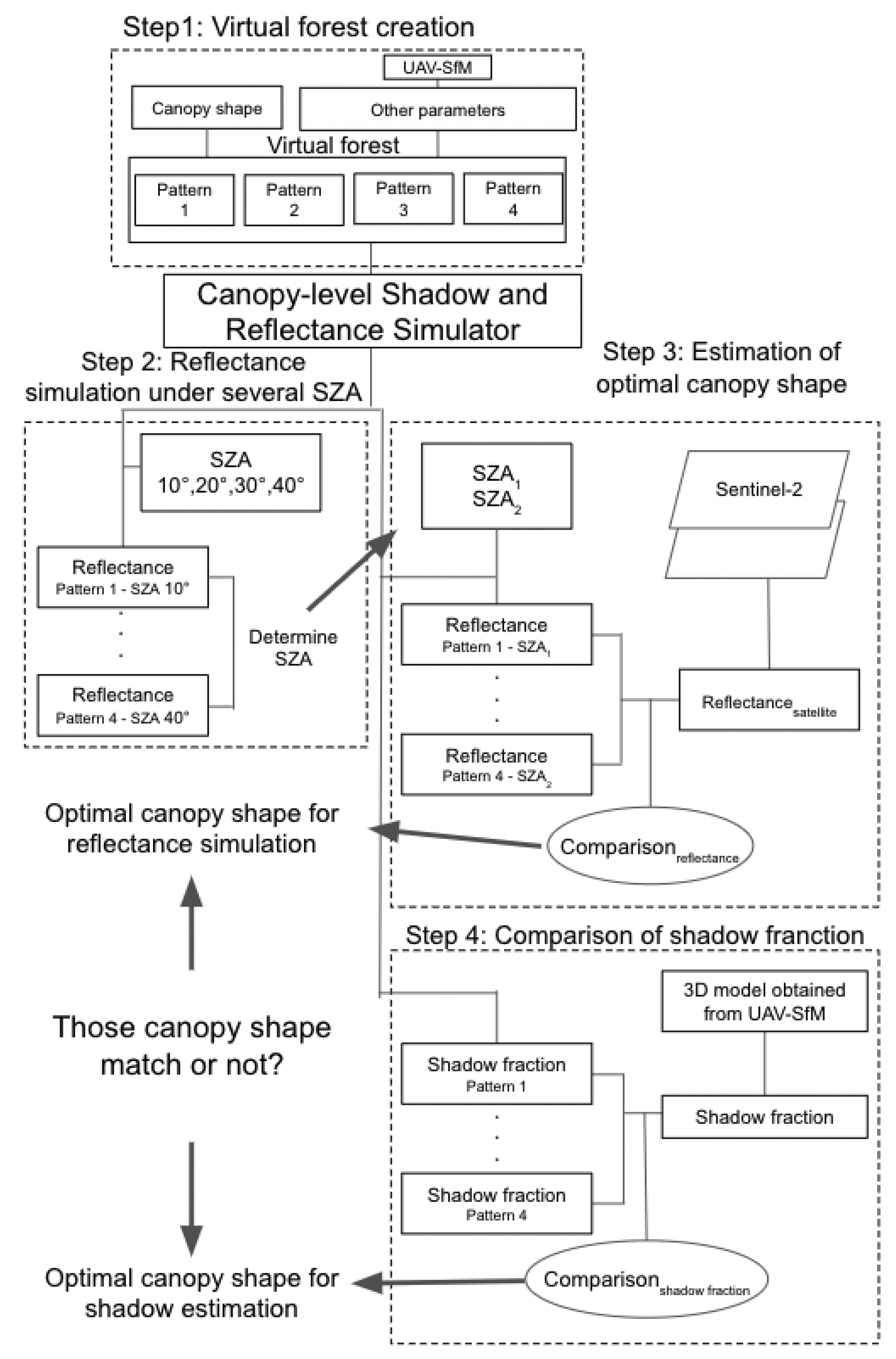
2.3. Research Flow
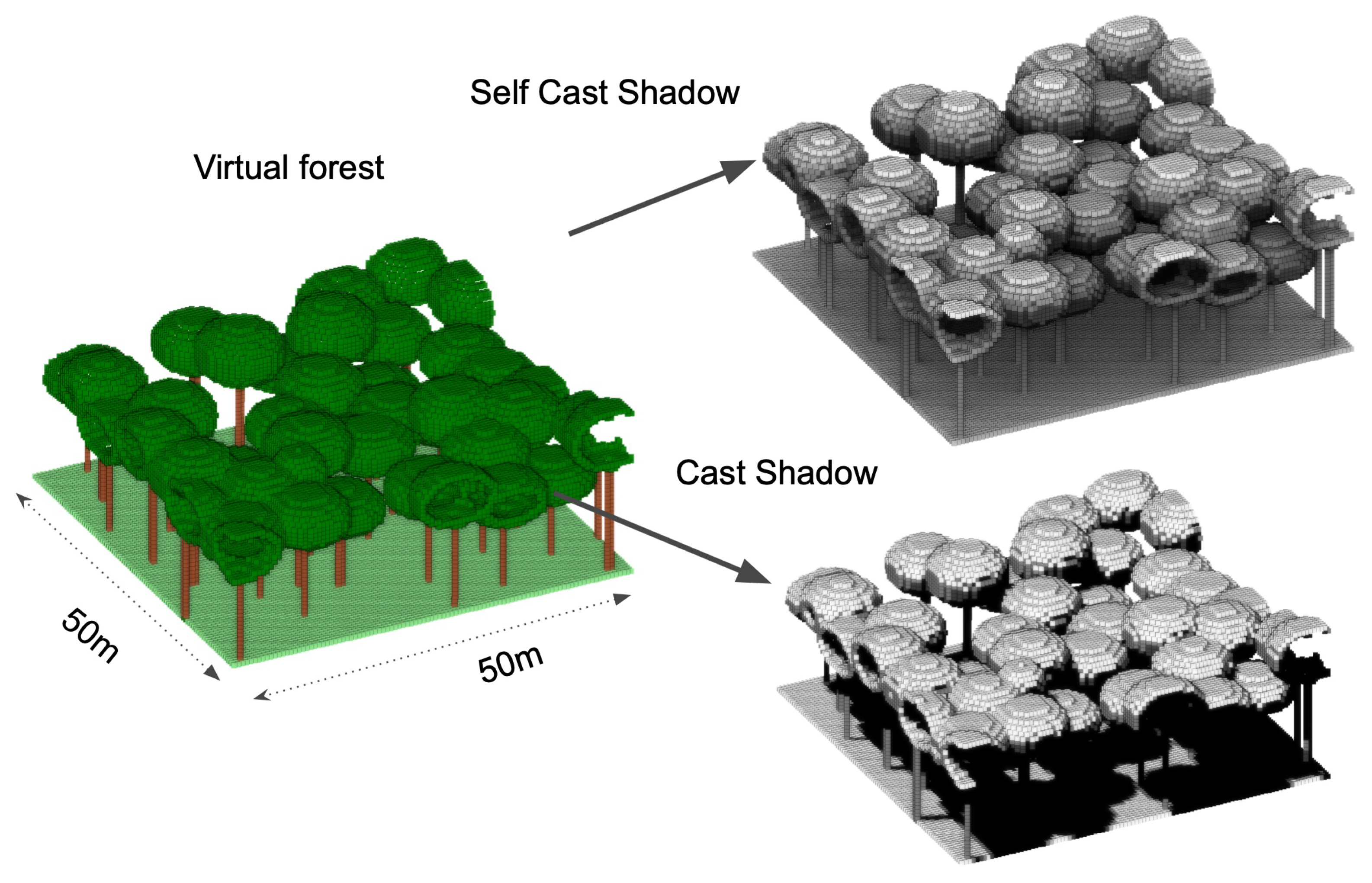
2.4. Description of Canopy-Level Shadow and Reflectance Simulator
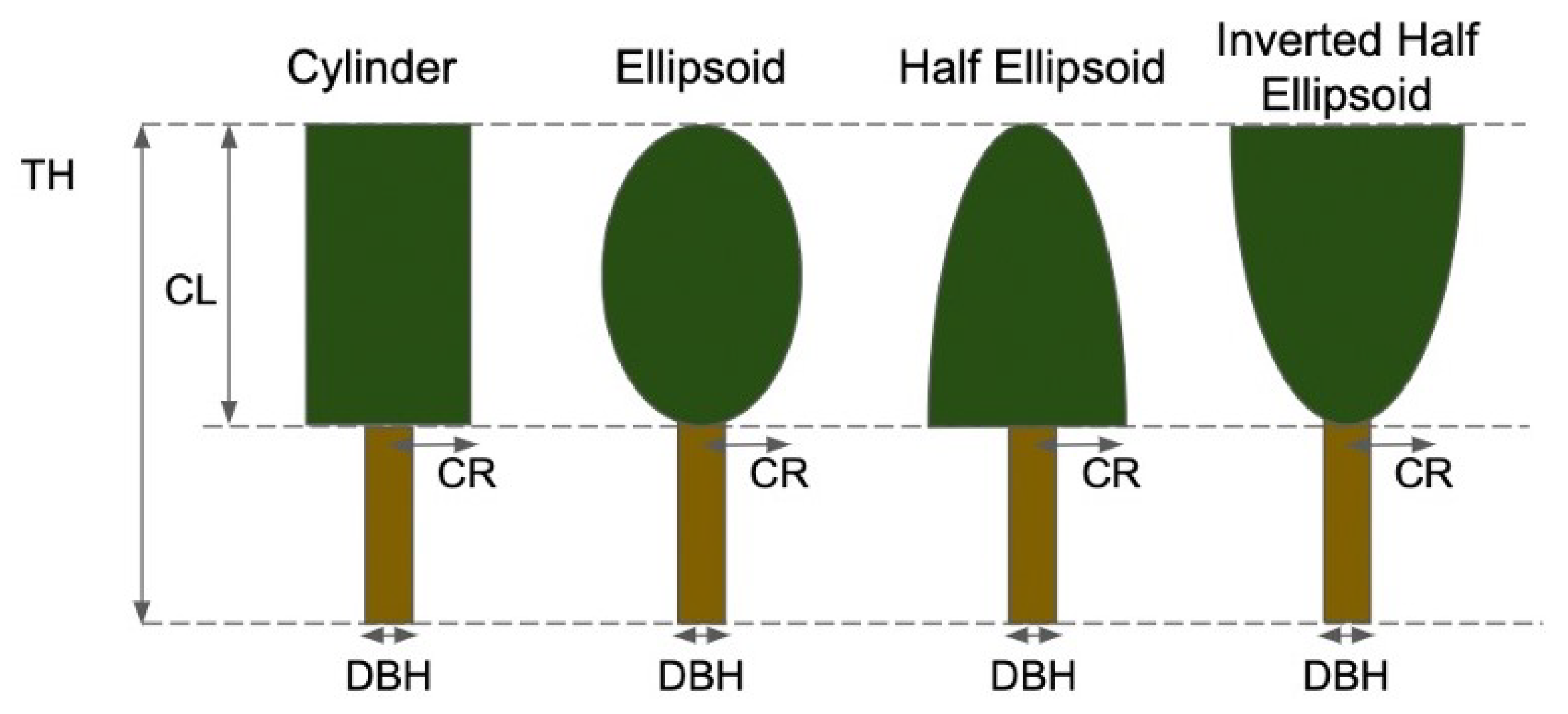
2.5. Forest Scene and Parameters
2.6. Performance Assessment of Estimated Reflectance and Shadow Fraction
3. Results
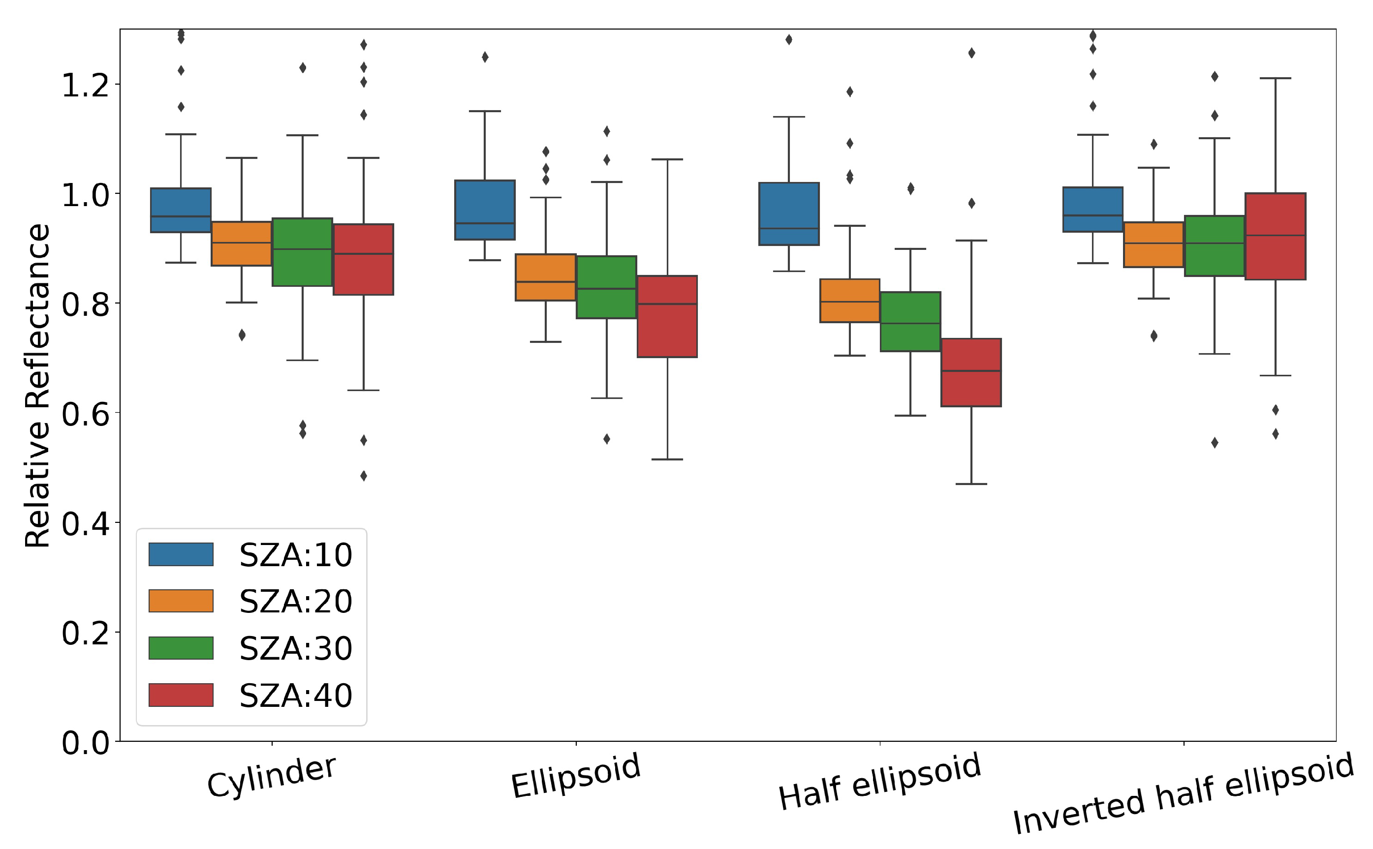
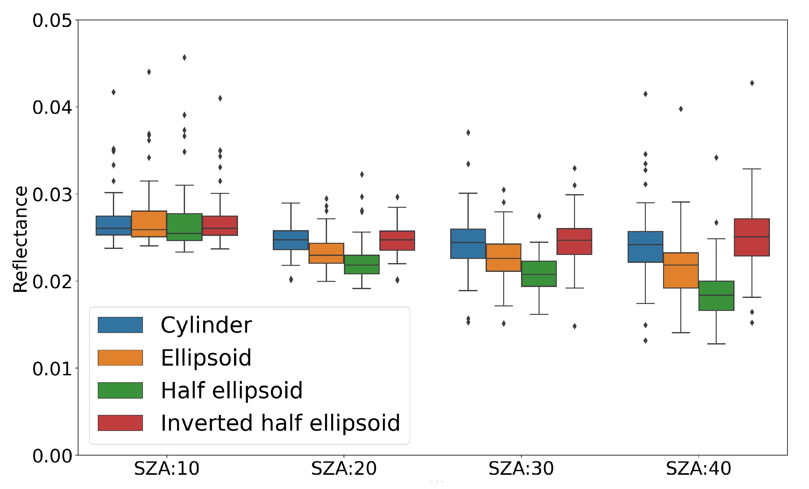
3.1. Reflectance Simulation under Several SZA
3.2. Determination of Optimal Canopy Shape and Comparison of Shadow Fraction
4. Discussion
4.1. The Effect of Canopy Shape on Reflectance Simulation
4.2. Limitations and Uncertainties of Reflectance Simulation
4.3. Future Work
5. Conclusions
Author Contributions
Funding
Data Availability Statement
Conflicts of Interest
References
- FAO. Assessment, Global Forest Resources 2020. Available online: https://www.fao.org/3/CA8753EN/CA8753EN.pdf (accessed on 10 November 2021).
- Beer, C.; Reichstein, M.; Tomelleri, E.; Ciais, P.; Jung, M.; Carvalhais, N.; Rödenbeck, C.; Arain, M.A.; Baldocchi, D.; Bonan, G.B.; et al. Terrestrial gross carbon dioxide uptake: Global distribution and covariation with climate. Science 2010, 329, 834–838. [Google Scholar] [CrossRef] [PubMed] [Green Version]
- Hengl, T.; Walsh, M.G.; Sanderman, J.; Wheeler, I.; Harrison, S.P.; Prentice, I.C. Global mapping of potential natural vegetation: An assessment of machine learning algorithms for estimating land potential. PeerJ 2018, 6, e5457. [Google Scholar] [CrossRef] [PubMed] [Green Version]
- Miura, T.; Nagai, S.; Takeuchi, M.; Ichii, K.; Yoshioka, H. Improved Characterisation of Vegetation and Land Surface Seasonal Dynamics in Central Japan with Himawari-8 Hypertemporal Data. Sci. Rep. 2019, 9, 15692. [Google Scholar] [CrossRef] [Green Version]
- Hashimoto, H.; Wang, W.; Dungan, J.L.; Li, S.; Michaelis, A.R.; Takenaka, H.; Higuchi, A.; Myneni, R.B.; Nemani, R.R. New generation geostationary satellite observations support seasonality in greenness of the Amazon evergreen forests. Nat. Commun. 2021, 12, 684. [Google Scholar] [CrossRef] [PubMed]
- Brooks, J.R.; Flanagan, L.B.; Varney, G.T.; Ehleringer, J.R. Vertical gradients in photosynthetic gas exchange characteristics and refixation of respired CO2 within boreal forest canopies. Tree Physiol. 1997, 17, 1–12. [Google Scholar] [CrossRef]
- Ellsworth, D.S.; Reich, P.B. Canopy structure and vertical patterns of photosynthesis and related leaf traits in a deciduous forest. Oecologia 1993, 96, 169–178. [Google Scholar] [CrossRef]
- Hilker, T.; Coops, N.C.; Schwalm, C.R.; Jassal, R.P.S.; Black, T.A.; Krishnan, P. Effects of mutual shading of tree crowns on prediction of photosynthetic light-use efficiency in a coastal Douglas-fir forest. Tree Physiol. 2008, 28, 825–834. [Google Scholar] [CrossRef]
- Kane, V.R.; Gillespie, A.R.; McGaughey, R.; Lutz, J.A.; Ceder, K.; Franklin, J.F. Interpretation and topographic compensation of conifer canopy self-shadowing. Remote Sens. Environ. 2008, 112, 3820–3832. [Google Scholar] [CrossRef]
- Chen, M. Comparison of 3D Tree Parameters. Master’s Thesis, Wageningen University and Research Centre, Wageningen, The Netherlands, 2013. [Google Scholar]
- Lefsky, M.A.; Harding, D.; Cohen, W.B.; Parker, G.; Shugart, H.H. Surface Lidar Remote Sensing of Basal Area and Biomass in Deciduous Forests of Eastern Maryland, USA. Remote Sens. Environ. 1999, 67, 83–98. [Google Scholar] [CrossRef]
- Potapov, P.; Li, X.; Hernandez-Serna, A.; Tyukavina, A.; Hansen, M.C.; Kommareddy, A.; Pickens, A.; Turubanova, S.; Tang, H.; Silva, C.E.; et al. Mapping global forest canopy height through integration of GEDI and Landsat data. Remote Sens. Environ. 2021, 253, 112165. [Google Scholar] [CrossRef]
- Simard, M.; Pinto, N.; Fisher, J.B.; Baccini, A. Mapping forest canopy height globally with spaceborne lidar. J. Geophys. Res. Biogeosci. 2011, 116, 4021. [Google Scholar] [CrossRef] [Green Version]
- Crowther, T.W.; Glick, H.B.; Covey, K.R.; Bettigole, C.; Maynard, D.S.; Thomas, S.M.; Smith, J.R.; Hintler, G.; Duguid, M.C.; Amatulli, G.; et al. Mapping tree density at a global scale. Nature 2015, 525, 201–205. [Google Scholar] [CrossRef] [PubMed]
- Nelson, R. Modeling forest canopy heights: The effects of canopy shape. Remote Sens. Environ. 1997, 60, 327–334. [Google Scholar] [CrossRef]
- Kobayashi, H.; Delbart, N.; Suzuki, R.; Kushida, K. A satellite-based method for monitoring seasonality in the overstory leaf area index of Siberian larch forest. J. Geophys. Res. Biogeosci. 2010, 115, 1002. [Google Scholar] [CrossRef] [Green Version]
- Ligot, G.; Ameztegui, A.; Courbaud, B.; Coll, L.; Kneeshaw, D. Tree light capture and spatial variability of understory light increase with species mixing and tree size heterogeneity. Can. J. For. Res. 2016, 46, 968–977. [Google Scholar] [CrossRef] [Green Version]
- Pisek, J.; Chen, J.M. Mapping forest background reflectivity over North America with Multi-angle Imaging SpectroRadiometer (MISR) data. Remote Sens. Environ. 2009, 113, 2412–2423. [Google Scholar] [CrossRef]
- Asner, G.P.; Braswell, B.H.; Schimel, D.S.; Wessman, C.A. Ecological Research Needs from Multiangle Remote Sensing Data. Remote Sens. Environ. 1998, 63, 155–165. [Google Scholar] [CrossRef]
- He, L.; Chen, J.M.; Pisek, J.; Schaaf, C.B.; Strahler, A.H. Global clumping index map derived from the MODIS BRDF product. Remote Sens. Environ. 2012, 119, 118–130. [Google Scholar] [CrossRef]
- Chen, J.M.; Leblanc, S.G. Four-scale bidirectional reflectance model based on canopy architecture. IEEE Trans. Geosci. Remote Sens. 1997, 35, 1316–1337. [Google Scholar] [CrossRef]
- Hasegawa, K.; Izumi, T.; Matsuyama, H.; Kajiwara, K.; Honda, Y. Seasonal change of bidirectional reflectance distribution function in mature Japanese larch forests and their phenology at the foot of Mt. Yatsugatake, central Japan. Remote Sens. Environ. 2018, 209, 524–539. [Google Scholar] [CrossRef]
- Fujiwara, T.; Takeuchi, W. Estimation of optimal crown coverage and canopy shape for shadow estimation on tropical moist broadleaf forest. ISPRS Ann. Photogramm. Remote Sens. Spat. Inf. Sci. 2021, 5, 211–217. [Google Scholar] [CrossRef]
- Hmimina, G.; Dufrêne, E.; Pontailler, J.Y.; Delpierre, N.; Aubinet, M.; Caquet, B.; de Grandcourt, A.; Burban, B.; Flechard, C.; Granier, A.; et al. Evaluation of the potential of MODIS satellite data to predict vegetation phenology in different biomes: An investigation using ground-based NDVI measurements. Remote Sens. Environ. 2013, 132, 145–158. [Google Scholar] [CrossRef]
- Myanmar Information Management Unit. Koppen–Geiger Climate Zones of Myanmar (1986–2010). Available online: https://themimu.info/sites/themimu.info/files/documents/Map_Koppen–Geiger_Climate_Zones_of_Myanmar_1986-2010_MIMU1548v01_17Jan2018_A4.pdf (accessed on 10 January 2021).
- Xu, N.; Tian, J.; Tian, Q.; Xu, K.; Tang, S. Analysis of Vegetation Red Edge with Different Illuminated/Shaded Canopy Proportions and to Construct Normalized Difference Canopy Shadow Index. Remote Sens. 2019, 11, 1192. [Google Scholar] [CrossRef] [Green Version]
- Gastellu-Etchegorry, J.P.; Demarez, V.; Pinel, V.; Zagolski, F. Modeling radiative transfer in heterogeneous 3-D vegetation canopies. Remote Sens. Environ. 1996, 58, 131–156. [Google Scholar] [CrossRef] [Green Version]
- Kobayashi, H.; Iwabuchi, H. A coupled 1-D atmosphere and 3-D canopy radiative transfer model for canopy reflectance, light environment, and photosynthesis simulation in a heterogeneous landscape. Remote Sens. Environ. 2008, 112, 173–185. [Google Scholar] [CrossRef]
- Qin, W.; Gerstl, S.A. 3-D Scene Modeling of Semidesert Vegetation Cover and its Radiation Regime. Remote Sens. Environ. 2000, 74, 145–162. [Google Scholar] [CrossRef]
- Fujiwara, T.; Takeuchi, W. Simulation of Sentinel-2 Bottom of Atmosphere Reflectance Using Shadow Parameters on a Deciduous Forest in Thailand. ISPRS Int. J. Geo-Inf. 2020, 9, 582. [Google Scholar] [CrossRef]
- Gueymard, C.A. Parameterized transmittance model for direct beam and circumsolar spectral irradiance. Sol. Energy 2001, 71, 325–346. [Google Scholar] [CrossRef]
- Wieczynski, D.J.; Díaz, S.; Durán, S.M.; Fyllas, N.M.; Salinas, N.; Martin, R.E.; Shenkin, A.; Silman, M.R.; Asner, G.P.; Bentley, L.P.; et al. Improving landscape-scale productivity estimates by integrating trait-based models and remotely-sensed foliar-trait and canopy-structural data. Ecography 2022, 2022, e06078. [Google Scholar] [CrossRef]
- Ma, X.; Huete, A.; Tran, N.N.; Bi, J.; Gao, S.; Zeng, Y. Sun-Angle Effects on Remote-Sensing Phenology Observed and Modelled Using Himawari-8. Remote Sens. 2020, 12, 1339. [Google Scholar] [CrossRef] [Green Version]
- Seelig, H.; Hoehn, A.; Stodieck, L.S.; Klaus, D.M.; Adams, W.W., III; Emery, W.J. The assessment of leaf water content using leaf reflectance ratios in the visible, near-, and short-wave-infrared. Int. J. Remote Sens. 2008, 29, 3701–3713. [Google Scholar] [CrossRef]
- Purves, D.W.; Lichstein, J.W.; Pacala, S.W. Crown Plasticity and Competition for Canopy Space: A New Spatially Implicit Model Parameterized for 250 North American Tree Species. PLoS ONE 2007, 2, e870. [Google Scholar] [CrossRef] [PubMed]
- Van Der Zee, J.; Lau, A.; Shenkin, A. Understanding crown shyness from a 3-D perspective. Ann. Bot. 2021, 128, 725–736. [Google Scholar] [CrossRef] [PubMed]
- Vepakomma, U.; St-Onge, B.; Kneeshaw, D. Spatially explicit characterization of boreal forest gap dynamics using multi-temporal lidar data. Remote Sens. Environ. 2008, 112, 2326–2340. [Google Scholar] [CrossRef]
- Loveland, T.R.; Reed, B.C.; Brown, J.F.; Ohlen, D.O.; Zhu, Z.; Yang, L.; Merchant, J.W. Development of a global land cover characteristics database and IGBP DISCover from 1 km AVHRR data. Int. J. Remote Sens. 2010, 21, 1303–1330. [Google Scholar] [CrossRef]


| Specification and Parameters | Value |
|---|---|
| Date | 30 September 2018 |
| Average Ground Sampling Distance | 4.5 cm |
| Flight elevation | 80 m |
| Number of images | 806 |
| Type of sensor onboard the UAV | Optical |
| Parameter | Value |
|---|---|
| Slope (degree) | |
| TH | X ~N () |
| Canopy shape | 4 pattern (shown in Figure 4) |
| CC (%) | 80% |
| CR (m) | X ~N () |
| CL (m) | Half of TH |
| DBH (m) | 0.3 |
| Overstory reflectance | Prospis articulata |
| Understory reflectance | Avena fatua |
| Sun Zenith Angle | , , , |
| Sun Azimuth Angle |
| Time | SAA | SZA |
|---|---|---|
| 08:00 | 98 | 61 |
| 10:00 | 115 | 33 |
| 12:00 | 181 | 16 |
| 13:00 | 244 | 34 |
| 14:00 | 261 | 62 |
| SZA (Degree) | Group1 | Group2 | Meandiff | p-adj | Lower | Upper | Reject |
|---|---|---|---|---|---|---|---|
| 10 | C | E | 0.0002 | 0.9 | −0.0019 | 0.0023 | False |
| C | HE | 0.0 | 0.9 | −0.0021 | 0.0021 | False | |
| C | IHE | −0.0 | 0.9 | −0.0021 | 0.002 | False | |
| E | HE | −0.0002 | 0.9 | −0.0023 | 0.0019 | False | |
| E | IHE | −0.0002 | 0.9 | −0.0023 | 0.0019 | False | |
| HE | IHE | −0.0 | 0.9 | −0.0021 | 0.002 | False | |
| 20 | C | E | −0.0015 | 0.0056 | −0.0026 | −0.0003 | True |
| C | HE | −0.0024 | 0.001 | −0.0035 | −0.0012 | True | |
| C | IHE | −0.0 | 0.9 | −0.0012 | 0.0011 | False | |
| E | HE | −0.0009 | 0.1661 | −0.002 | 0.0002 | False | |
| E | IHE | 0.0014 | 0.008 | 0.0003 | 0.0025 | True | |
| HE | IHE | 0.0023 | 0.001 | 0.0012 | 0.0034 | True | |
| 30 | C | E | −0.0018 | 0.0212 | −0.0034 | −0.0002 | True |
| C | HE | −0.0036 | 0.001 | −0.0053 | −0.002 | True | |
| C | IHE | 0.0 | 0.9 | −0.0016 | 0.0016 | False | |
| E | HE | −0.0018 | 0.0191 | −0.0034 | −0.0002 | True | |
| E | IHE | 0.0018 | 0.0181 | 0.0002 | 0.0035 | True | |
| HE | IHE | 0.0037 | 0.001 | 0.0021 | 0.0053 | True | |
| 40 | C | E | −0.0026 | 0.0153 | −0.0049 | −0.0004 | True |
| C | HE | −0.0057 | 0.001 | −0.008 | −0.0035 | True | |
| C | IHE | 0.0007 | 0.8461 | −0.0016 | 0.0029 | False | |
| E | HE | −0.0031 | 0.0027 | −0.0054 | −0.0008 | True | |
| E | IHE | 0.0033 | 0.0011 | 0.0011 | 0.0056 | True | |
| HE | IHE | 0.0064 | 0.001 | 0.0041 | 0.0087 | True |
| Season | Date | SAA | SZA |
|---|---|---|---|
| 1 | 13 April 2019 | 108.7 | 21.3 |
| 28 April 2019 | 129.9 | 22.4 | |
| 12 April 2020 | 108.9 | 21.4 | |
| 22 April 2020 | 100.0 | 19.7 | |
| 7 May 2020 | 86.3 | 18.5 | |
| 2 | 9 December 2019 | 155.1 | 43.3 |
| 14 December 2019 | 154.7 | 43.9 | |
| 24 December 2019 | 153.4 | 44.6 | |
| 13 December 2020 | 154.7 | 43.9 | |
| 28 December 2020 | 152.6 | 44.7 |
| Canopy Shape | RMSE | |
|---|---|---|
| Reflectance Simulation | Shadow Simulation | |
| C | 0.542 | 0.125 |
| E | 0.456 | 0.035 |
| HE | 0.385 | 0.032 |
| IHE | 0.537 | 0.129 |
Publisher’s Note: MDPI stays neutral with regard to jurisdictional claims in published maps and institutional affiliations. |
© 2022 by the authors. Licensee MDPI, Basel, Switzerland. This article is an open access article distributed under the terms and conditions of the Creative Commons Attribution (CC BY) license (https://creativecommons.org/licenses/by/4.0/).
Share and Cite
Fujiwara, T.; Takeuchi, W. Modeling Shadow with Voxel-Based Trees for Sentinel-2 Reflectance Simulation in Tropical Rainforest. Remote Sens. 2022, 14, 4088. https://doi.org/10.3390/rs14164088
Fujiwara T, Takeuchi W. Modeling Shadow with Voxel-Based Trees for Sentinel-2 Reflectance Simulation in Tropical Rainforest. Remote Sensing. 2022; 14(16):4088. https://doi.org/10.3390/rs14164088
Chicago/Turabian StyleFujiwara, Takumi, and Wataru Takeuchi. 2022. "Modeling Shadow with Voxel-Based Trees for Sentinel-2 Reflectance Simulation in Tropical Rainforest" Remote Sensing 14, no. 16: 4088. https://doi.org/10.3390/rs14164088
APA StyleFujiwara, T., & Takeuchi, W. (2022). Modeling Shadow with Voxel-Based Trees for Sentinel-2 Reflectance Simulation in Tropical Rainforest. Remote Sensing, 14(16), 4088. https://doi.org/10.3390/rs14164088