Article

Precipitation Dominates the Distribution of Species Richness on the Kunlun–Pamir Plateau

1
Key Laboratory of Smart City and Environment Modelling of Higher Education Institute, College of Resources and Environment Sciences, Xinjiang University, Urumqi 830046, China
2
State Key Laboratory of Desert and Oasis Ecology, Xinjiang Institute of Ecology and Geography, Chinese Academy of Sciences, Urumqi 830011, China
3
University of Chinese Academy of Sciences, Beijing 100049, China
4
Department of Geography, Ghent University, 9000 Ghent, Belgium
5
Sino-Belgian Joint Laboratory of Geo-Information, Urumqi 830011, China
6
China-Pakistan Joint Research Centre on Earth Sciences, CAS-HEC, Islamabad 45320, Pakistan
7
Research Centre for Ecology and Environment of Central Asia, Chinese Academy of Sciences, Urumqi 830011, China
8
College of Earth and Environmental Sciences, Lanzhou University, Lanzhou 730000, China
9
Sino-Belgian Joint Laboratory of Geo-Information, 9000 Ghent, Belgium
*
Author to whom correspondence should be addressed.
Remote Sens. 2022, 14(24), 6187; https://doi.org/10.3390/rs14246187
Submission received: 12 October 2022 / Revised: 30 November 2022 / Accepted: 2 December 2022 / Published: 7 December 2022
(This article belongs to the Special Issue Application of Earth Observation for Monitoring Biodiversity)

Abstract

:
The Kunlun–Pamir Plateau is a globally irreplaceable biodiversity reserve, yet it is still unclear what causes the distribution of species richness. Here, we relied on the productivity and the water–energy dynamics hypotheses to investigate the distribution pattern of species richness (and its determinants) in the Kunlun–Pamir Plateau. The productivity hypothesis is mainly based on five MODIS products (NDVI, EVI, FPAR, LAI and GPP), which were calculated for three Dynamic Habitat Indices (DHIs): (1) cumulative productivity (CumDHI), (2) minimum productivity (MinDHI) and (3) intra-annual variation productivity (VarDHI). The CumDHI was applied to assess whether or not more energy has a higher species richness value. The MinDHI was used to determine and evaluate the higher minimums, leading to a higher species richness. The VarDHI was the annual variation value in productivity and was utilized to assess if the reduced intra-annual variability triggers a higher species richness. We found that the DHIs based on the FPAR correlated slightly higher with the mammal, bird, breeding bird and non-breeding bird richness (than those based on the other four DHIs, and the values were 0.24, 0.25, 0.24 and 0.01, respectively). The correlation between the climate variables and the mammals, birds, breeding birds and non-breeding birds was bigger at 0.24, 0.54, 0.54 and 0.02, respectively, and was mainly dominated by the precipitation-related climatic factors. The water–energy dynamic hypothesis is better suited to the Kunlun–Pamir Plateau than the productivity hypothesis. Our results might provide valuable information regarding the biodiversity conservation in this region.

Graphical Abstract

1. Introduction

The high value species richness means a rich regional biodiversity. The research of species richness is the basis for constructing evolutionary, ecological models and conservation strategies [1,2]. The global species richness has decreased during the last decades [3], and this trend will continue [4]. Several theoretical hypotheses, such as the productivity hypothesis [5,6], water–energy dynamic hypothesis [7,8], ambient energy hypothesis [9,10], cold tolerance hypothesis [8,11] and the metabolic theory of ecology [12,13,14], were used to explain the distribution patterns of species richness. Among those hypotheses, the productivity hypothesis and the water–energy dynamic hypothesis were the most widely used. The productivity hypothesis suggests that the higher the productivity, the higher the species richness [5,6,15,16]. The main idea of the water–energy dynamics hypothesis (sometimes referred to as the moisture hypothesis) showed that the large-scale patterns of species richness are determined by a combination of water and energy [7]. The energy in this hypothesis is usually expressed by the potential evapotranspiration, temperature or moisture. The water is generally referred to as liquid water and is commonly expressed as the annual rainfall of a region [7,17]. Some studies have applied climate data to present energy and moisture variables [18,19].
Satellite observations provide a rich, long-time series of vegetation productivity products. They can be used to test the productivity hypothesis [20,21]. The Moderate Resolution Imaging Spectroradiometer (MODIS) data collected by NASA’s Terra and Aqua satellites offered various products. This could be utilized for species richness assessments at different scales and include the vegetation indices, such as the Normalized Difference Vegetation Index (NDVI) and Enhanced Vegetation Index (EVI)), Leaf Area Index (LAI) and Fraction of absorbed Photosynthetically Active Radiation (FPAR), as well as Gross Primary Productivity (GPP). The most suitable productivity products vary from region to region. The NDVI and EVI belong to the same MODIS vegetation dataset. The NDVI is the best indicator of vegetation growth status and vegetation cover; however, overfitting exists in densely vegetated areas due to nonlinear transformations. The EVI improves on NDVI saturation. The FPAR and LAI are based on reflectance values of up to seven MODIS spectral bands, while the NDVI and EVI are based on two and three bands, respectively, so the FPAR and LAI provide a closer proxy for vegetation productivity than the NDVI and EVI. GPP products are mainly calculated using FPAR, light and effective radiation (PAR), as well as other surface meteorological data from remote sensing inversion using a light energy utilization model, which is good information for monitoring vegetation growth. Five MODIS products allow a multifaceted and more comprehensive analysis of their relationship with species richness [22]. The Dynamic Habitat Indices (DHIs) based on the productivity hypothesis theory can be calculated from the MODIS products to demonstrate the distribution of species richness [23,24]. It has been proven that these correlate well with the species richness [22,25,26]. The DHIs comprise three indicators: the cumulative annual productivity (CumDHI), minimum productivity (MinDHI) and productivity variation (VarDHI). A good correlation between these indices and the species richness was confirmed on the local and global scales [22,26,27,28,29,30,31,32]. For example, the biodiversity in China has been detected by the FPAR-derived DHIs [31]. In the United States, the bird species richness correlated with the FPAR-derived DHIs on grasslands, while it denoted a better correlation with the LAI-derived DHIs on woodlands [22]. In Russia, FPAR-derived DHIs combined with climatic variables seemed promising to predict the abundance of large ungulates such as moose [32]. On a global scale, the multiple regression used GPP-derived DHIs that also adequately described the distribution of species richness [26]. The species richness was simultaneously impacted by a combination of various factors and processes but varied significantly across the scales and regions.
The Kunlun–Pamir Plateau is adjacent to the Tibetan Plateau, which constitutes the second-highest plateau in the world. It is located in the arid zone and is also an irreplaceable global biodiversity reserve. Its substratum is a complex, sensitive and vulnerable area for the global climate and environmental change [33]. Additionally, it has a continental alpine environment with long winters, a scarce precipitation, mainly bare land and desert grasslands. However, there is still a lack of research on the spatial distribution of species richness and their causes at this plateau.
Our goal was to use the productivity hypothesis based on DHIs and the water–energy dynamic hypothesis based on bioclimatic factors to explain the species richness distribution of the Kunlun–Pamir Plateau. Specifically, we sought (1) to derive and describe the DHIs at a 500 m resolution from the MODIS vegetation products on the Kunlun–Pamir Plateau and (2) to analyze the applicability of these two hypotheses in the area.

2. Data and Methods

2.1. Data

2.1.1. MODIS Data

The MODIS products used to calculate the DHIs included the NDVI, EVI, FPAR, LAI and GPP in both 8- and 16-day composites and at a 500 m resolution (Table 1). All products from 2001 to 2020 were downloaded from the Application for Extracting and Exploring the Analysis Ready Samples (AEEARS) https://appeears.earthdatacloud.nasa.gov/ (accessed on 14 July 2022). These are all related to the vegetation productivity and could be used to validate the application of the productivity hypothesis [22,25,26].

2.1.2. Species Richness

The species richness data were downloaded from the website BiodiversityMapping.org (https://biodiversitymapping.org/index.php/download/ (accessed on 7 August 2022)) [34,35,36]. They are also from the IUCN [37] (http://www.iucnredlist.org (accessed on 7 August 2022)) and Birdlife International (http://datazone.birdlife.org/species/requestdis (accessed on 7 August 2022)) [38]. The maps currently comprise mammals, birds, breeding birds and non-breeding birds. Its spatial resolution is 10 × 10 km with the Eckert IV equal-area projection. Maps represent native extant species only.

2.1.3. Climatic Data
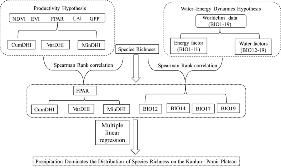
The climatic data are used from Worldclim version 2.1 with a spatial resolution of 30″ and include 19 bioclimatic variables (https://www.Worldclim.org/data/Worldclim21.html (accessed on 24 May 2022)) for 1970–2000. It was released in January 2020. The first eleven variables (BIO1–11) were applied to characterize the energy, and the last eight ones (BIO12–19) were selected to describe the water factors. The variation in vegetation was also impacted by the climate variables (Table 2).

2.2. Methods

2.2.1. Calculation of the DHIs

First, the 8-day and 16-day NDVI, EVI, FPAR and LAI products were synthesized into monthly data using the maximum synthesis method [22,26,39]. Then, the CumDHI, MinDHI and VarDHI were calculated for these indices from 2001 to 2021.
The CumDHI is the sum of the production values for one year. Since it signifies the number of annually available resources that could provide animals with resources such as food, it might indirectly indicate the species abundance [40]. Here, the calculation of the DHI for FPAR is applied as an example, and its equation is shown below:
CumDHI = month MAX layer ,   FPAR
where the layer refers to the monthly data.
The MinDHI stands for the minimum extent of vegetation cover in one year and represents the minimum capacity within one year. It could denote the minimum accommodation of food and habitat resources during a year [40]. It is calculated by means of the following equation:
MinDHI = MIN { ( MAX layer , Fpar ) month }
where VarDHI stands for the variation of the production values in one year. It refers to the natural resources associated with the habitat quality, such as food, water, nutrient substances, etc. within the year, and it might reveal the characteristics of the organisms’ activity trajectory [28]. The following equation calculates the VarDHI:
VarDHI = STD { ( MAX layer , FPAR ) month }
where MAX layer , FPAR refers to the maximum FPAR value for one month, and the month indicates the 12 months of the year. MIN and STD represent the minimum and standard deviation of the maximum monthly value of FPAR for one year. The above-mentioned equations were applied to the NDVI, EVI, FPAR and LAI. The GPP was computed by replacing the maximum values with the cumulative values in the three equations.

2.2.2. Statistical Analysis

The Spearman correlation was utilized to quantify the degree of interchangeability between the same MODIS products-based DHI and different MODIS products. In order to verify whether or not climate variables impacted the DHIs (CumDHI, MinDHI and VarDHI), we performed a correlation analysis of the DHIs with 19 Bioclim variables. All correlation analyses were based on a random sample of 10,000 of the 1 km DHIs and bioclimatic variable pixels with the “no data” set to zero [22,26].
We computed the Spearman rank correlations of species richness, DHIs and Bioclim variables, and scatter plots were produced for visualization purposes. Multiple linear regression models estimated the dependent variables using the most available combinations of various independent variables to make the results more trustworthy. We conducted multiple linear regression analyses to predict the species richness based on two hypotheses, and the relative contribution of each model was conducted by hierarchical partitioning analyses using the R package hier.part [41]. The analysis was based on a sample of 10,000 of the 10 km resampled DHIs and Bioclim variables. The root mean square error (RMSE) and the adjusted coefficient of determination (R2 adj) were used to evaluate the overall predictive power of a model under 95% confidence intervals.

3. Results

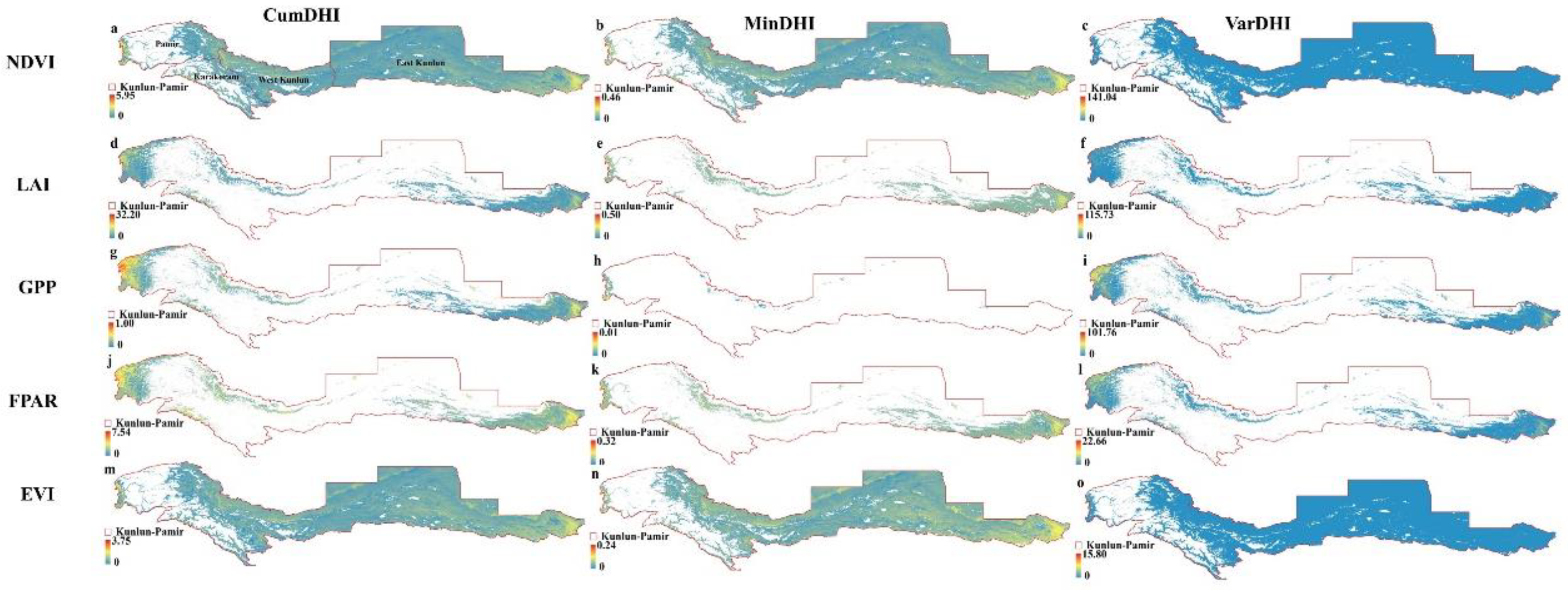
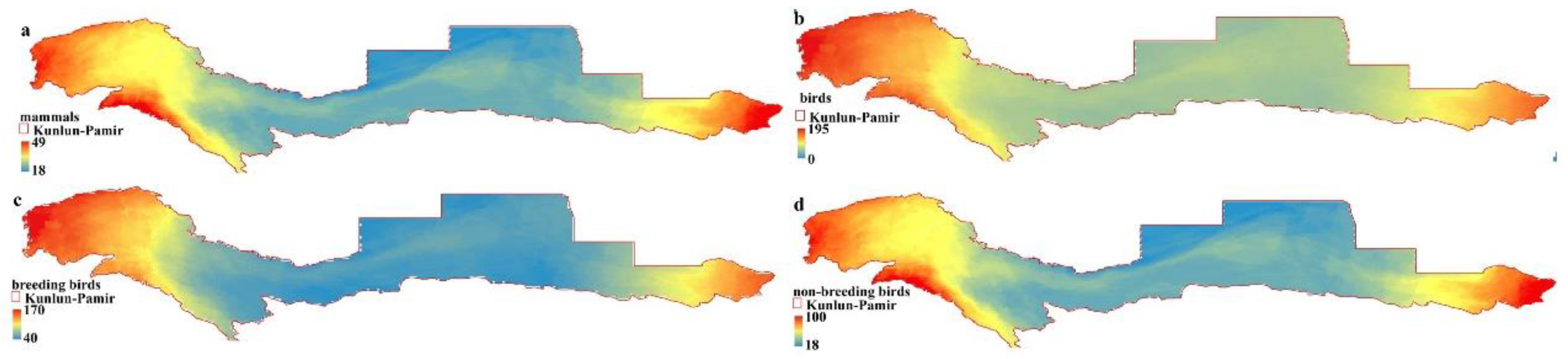
3.1. Distribution Patterns of DHIs

In the Kunlun–Pamir Plateau region, the spatial changes in the distribution of the cumulative DHI, minimum DHI and variation DHI values are rather insignificant. However, various MODIS products demonstrated different distribution patterns (Figure 1a–f). The DHIs of the same MODIS vegetation dataset indicated positive correlations. The correlation between the cumulative DHIs and the minimum DHI was moderately intense, except in the case of GPP, in which the correlation between the cumulative DHI and minimum DHI was rather small (0.23). The Spearman rank correlation ranged from 0.50 to 1. The correlations of variation DHIs with a cumulative DHI and minimal DHI were 0.43 to 1 and 0.21 to 0.81, respectively. The correlation between the GPP variation DHI and minimal DHI was 0.21 (Figure 2).
The DHI correlations from different vegetation datasets were uneven. Some of correlations were also nonlinear (Figure 2). The Spearman rank correlations of the same vegetation products (e.g., NDVI- and EVI-based DHIs) were higher than the ones between the DHIs based on different vegetation products (e.g., FPAR- and GPP-based DHIs). The highest correlations values were noticed between the FPAR- and LAI-based DHIs (from 0.78 for the minimum DHI to 1 for the cumulative and variation DHI). The correlations between the cumulative and variation DHIs based on the GPP, FPAR and LAI were also substantial (Figure 2 and Figure 3). The GPP-based DHI correlated the least with the DHI based on other vegetation products, except the cumulative and variation LAI, with a minimum DHI correlation of 0.11.
Due to the high correlation between FPAR-based DHIs and species richness, we selected FPAR-DHIs for the subsequent work analysis (Table 3 and Tables S1–S4). Most of the correlations between the FPAR-based DHIs and the climate dataset were weak (Figure 4), indicating that the DHIs possibly provide various information. The highest Spearman rank correlation value with the energy factor was −0.13 (BIO4, Temperature Seasonality) during the cumulative DHIs. Regarding the water factor, the highest Spearman rank correlation measured 0.07 (BIO13, the wettest month).

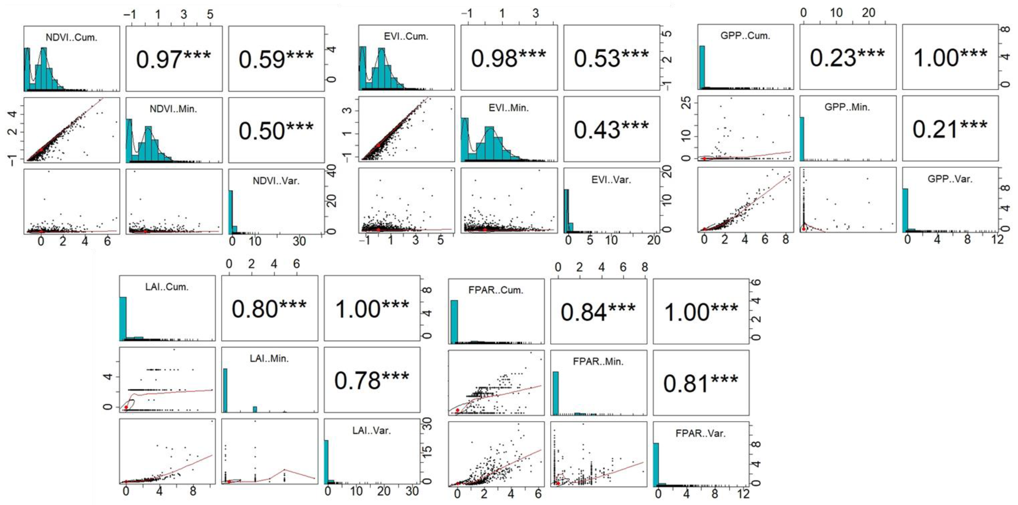
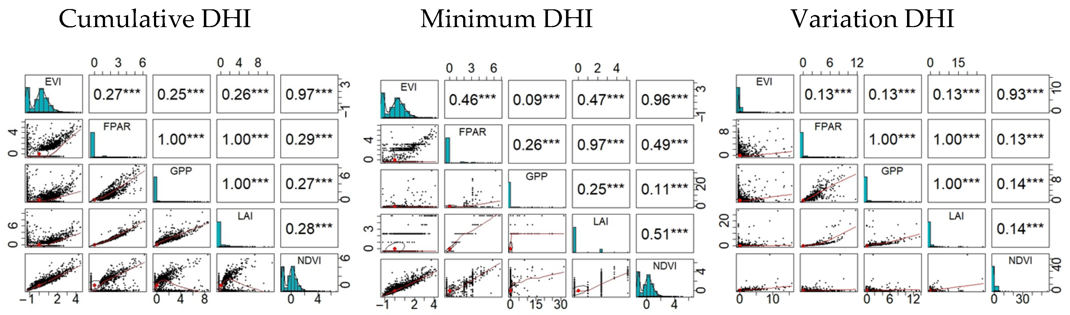
3.2. Species Richness and Productivity Hypothesis

The high density of a species is mainly spread in the marginal regions of the Kunlun–Pamir Plateau, characterized by relatively small areas (Figure 5). The dense distribution of species is primarily detected in the frontier areas of the Kunlun–Pamir Plateau, with relatively small but insignificant differences in species’ abundance in the central region (Figure 5). The species richness correlated positively with the cumulative DHI based on the FPAR for all four categories, with the Spearman rank correlation coefficients amounting to 0.36, 0.39, 0.39 and 0.08 for mammals, birds, breeding birds and non-breeding birds, respectively. However, there was also a considerable dispersion noticeable. The minimum DHI based on the FPAR predicted that the species richness was higher when the minimum DHI based on the FPAR was larger. In this case, the positive correlation coefficients were 0.19, 0.22, 0.22 and 0.04 for mammals, birds, breeding birds and non-breeding birds, respectively. The scatter plots of the minimum DHI based on the FPAR versus the species richness for the four taxa were similar to those of the cumulative DHI based on the FPAR and variation DHI based on the FPAR. The variation DHI based on the FPAR predicted that the species richness would be higher when there was less variability. However, because most parts of the Kunlun–Pamir Plateau region are bare land and desert steppe, the species richness was higher when the environmental conditions were more variable. Indeed, the variability in the Kunlun–Pamir Plateau region correlated positively with the species richness for all four taxa, with positive correlation coefficients of 0.36, 0.4, 0.4 and 0.08 for mammals, birds, breeding birds and non-breeding birds, respectively. This implies that, for all four taxa, high values of the variability DHI based on the FPAR indicate a high species richness variation.
Furthermore, the three DHIs based on the FPAR complement each other (Figure 6 and Table 3). A hierarchical partitioning analysis of the multiple regression models showed that all three DHIs based on the FPAR contributed considerably to the explanation of the overall variability in species richness. The cumulative DHI based on the FPAR was the most critical variable in each regression model, followed by the varDHI based on the FPAR and MinDHI based on the FPAR. According to the regression models, birds demonstrate the most explanatory power, and non-breeding birds exhibit the least explanatory power among these four categories (Figure 6).

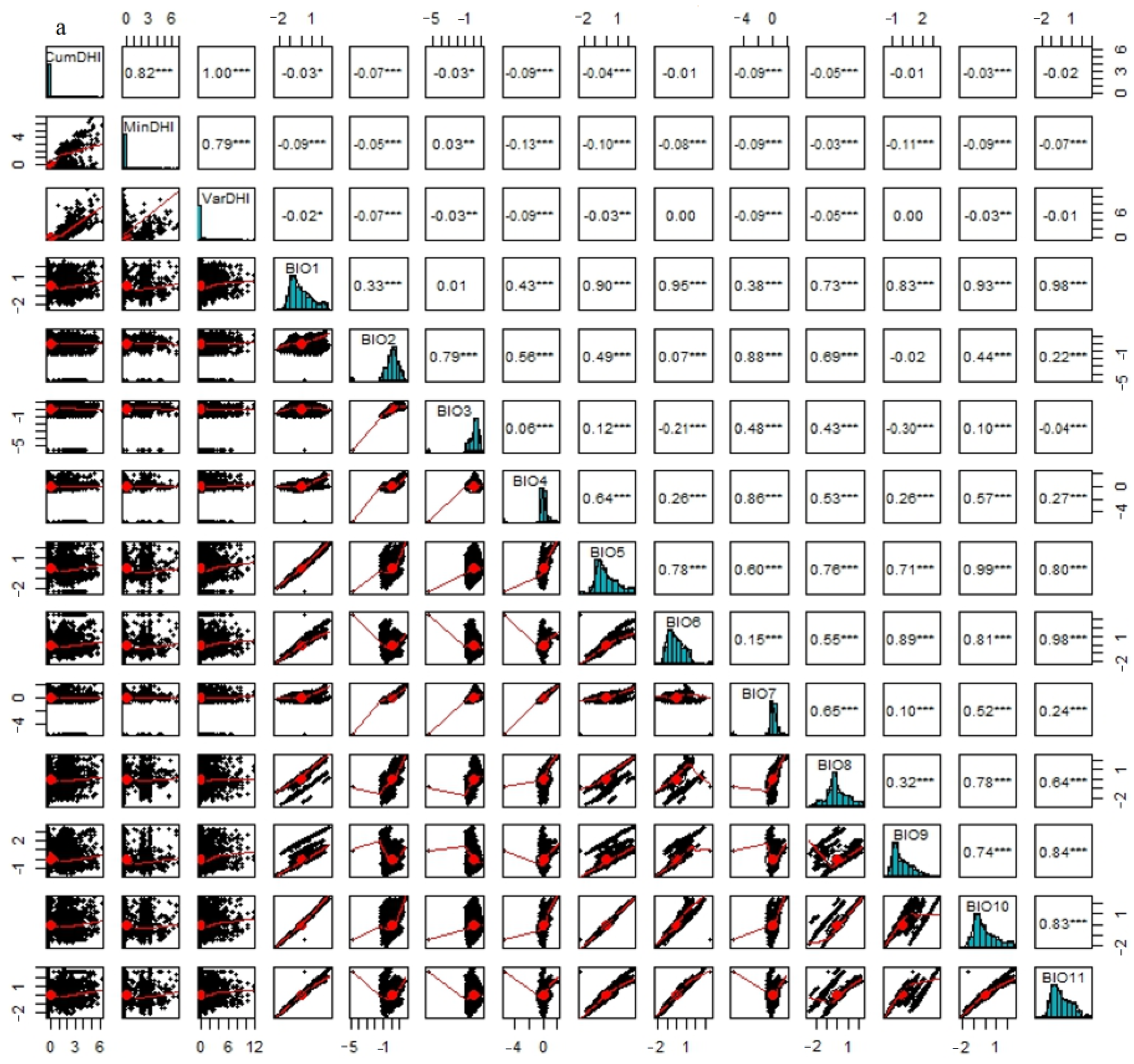
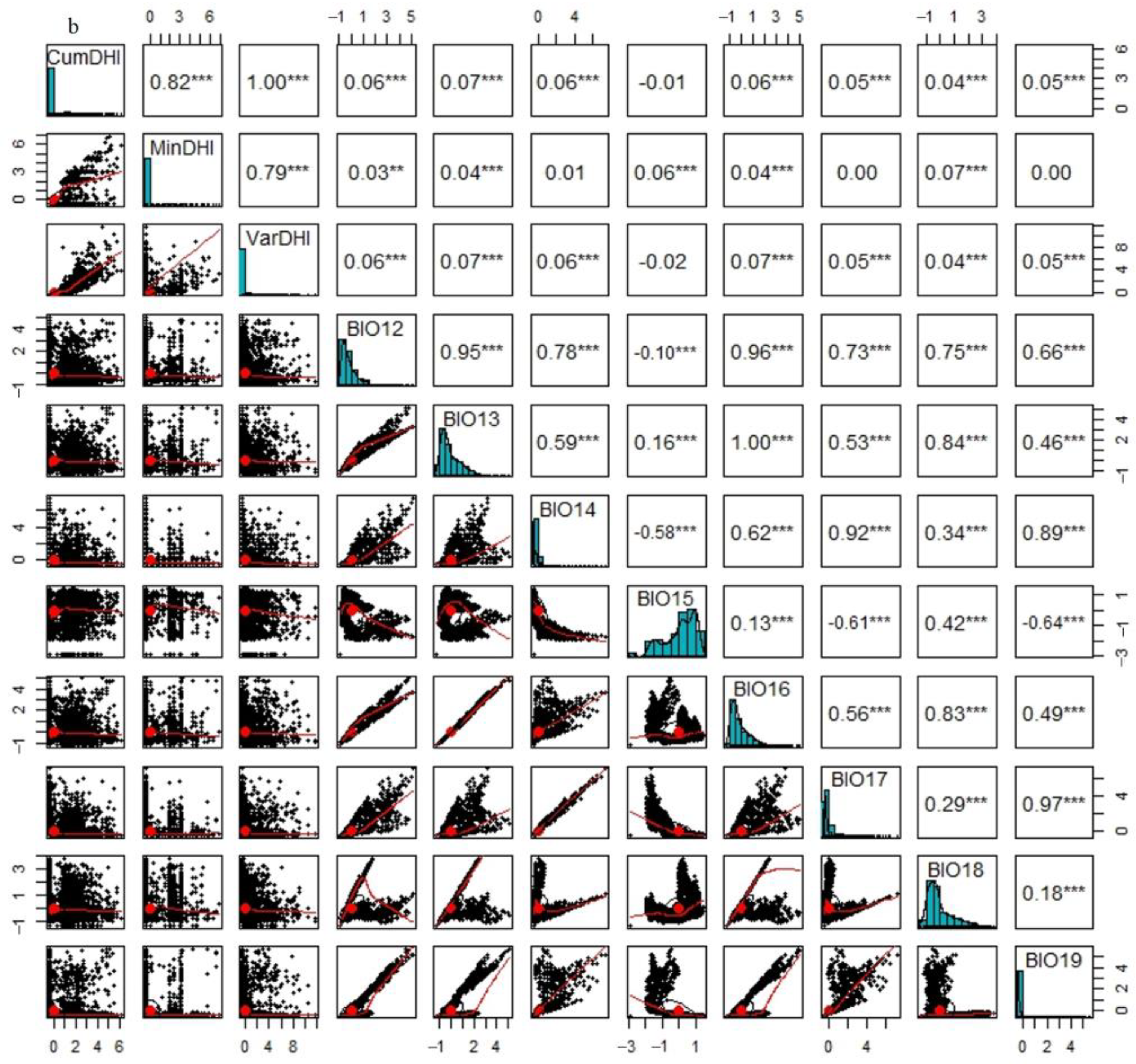
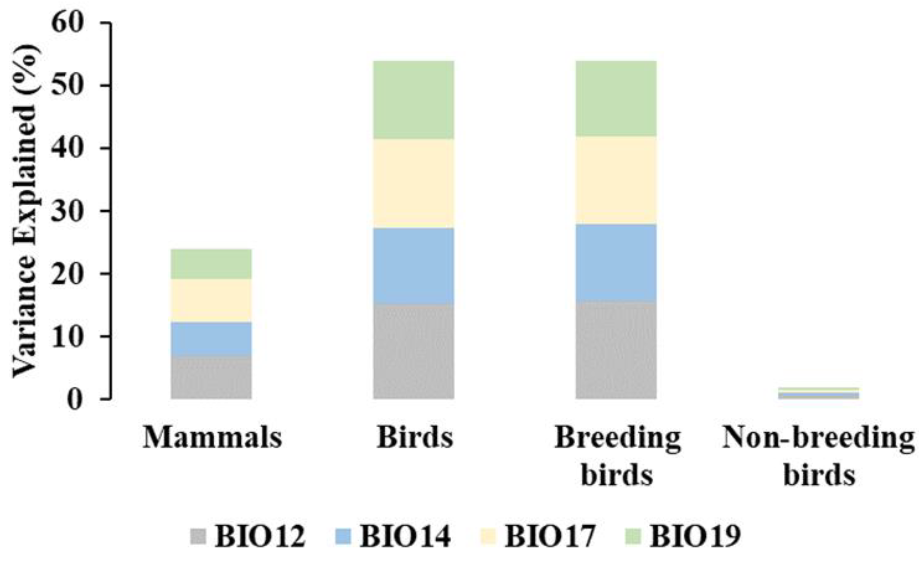
3.3. Species Richness and the Water–Energy Dynamics Hypothesis

The climatic factors affected the distribution of the species richness in the Kunlun–Pamir Plateau region (Table 4). Among the bioclimatic variables, BIO12, -14, -17 and -19 denoted the highest rank correlation coefficients in species richness. Although the differences between the four variables were not statistically significant, BIO17 demonstrated the highest rank correlation coefficient regarding the species richness. Spearman’s rank correlation coefficients with the BIO17 Precipitation of the Driest Quarter measured 0.61, 0.73, 0.72 and 0.14 for mammals, birds, breeding birds and non-breeding birds, respectively. The higher BIO17 corresponded to a larger species richness. Among the four taxa, the birds and breeding birds demonstrated more substantial Spearman rank correlation coefficients with climate factors as compared to the mammals and non-breeding birds.
We noticed that all BIOs (12, 14, 17 and 19) contributed more to the overall richness variability in the multiple linear regression. A hierarchical partitioning analysis of the multiple regression models showed that the four bioclimatic variables’ influence complemented the definition of the overall richness variability. BIO17 identified as being the most important for mammals and birds, while BIO14 was the most striking for the breeding birds and non-breeding birds. The minimum DHI was the least effective for all models. Among the significant taxa, the breeding bird’s regression model explained most of the variation in species richness (Figure 7 and Table 4).

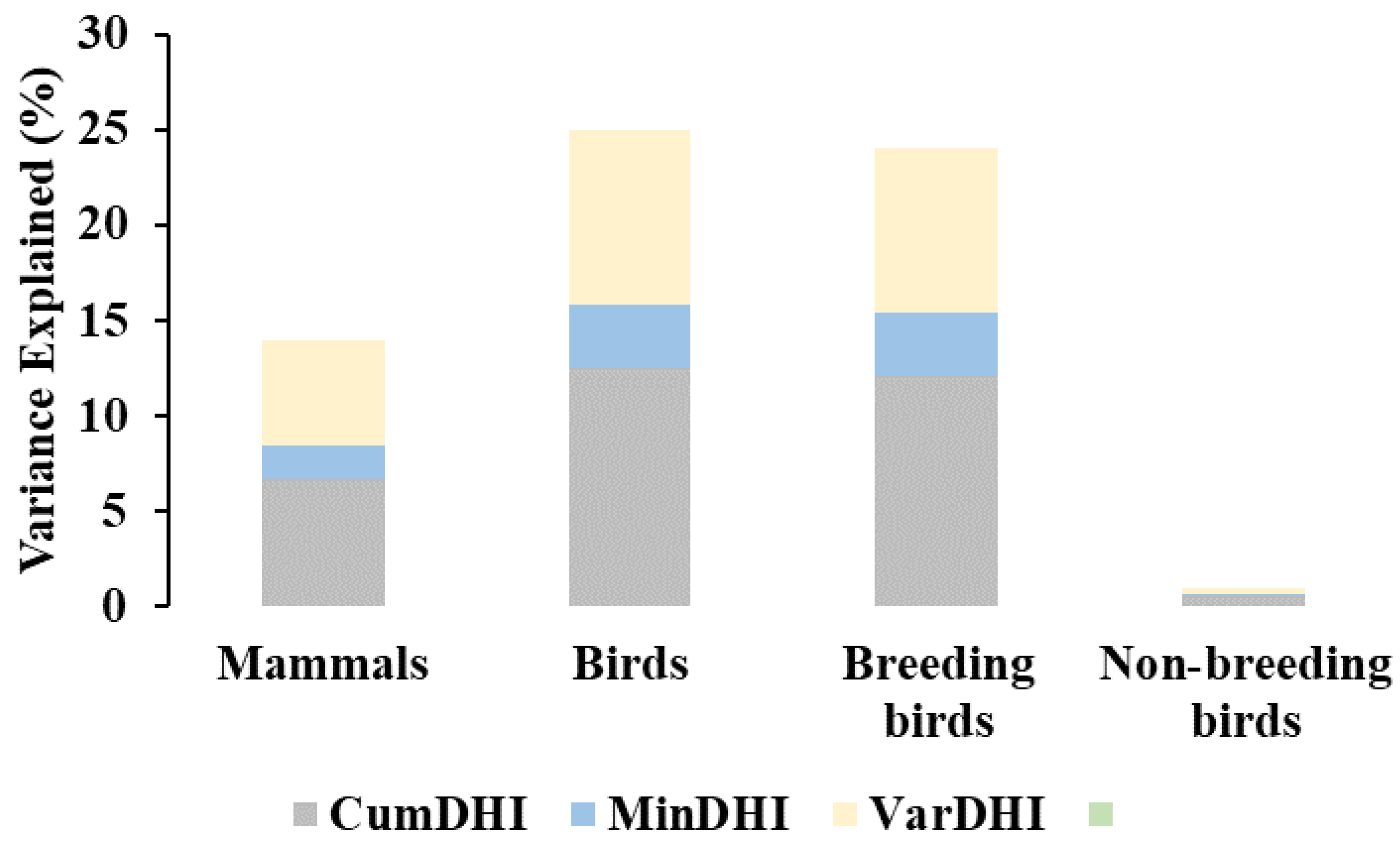
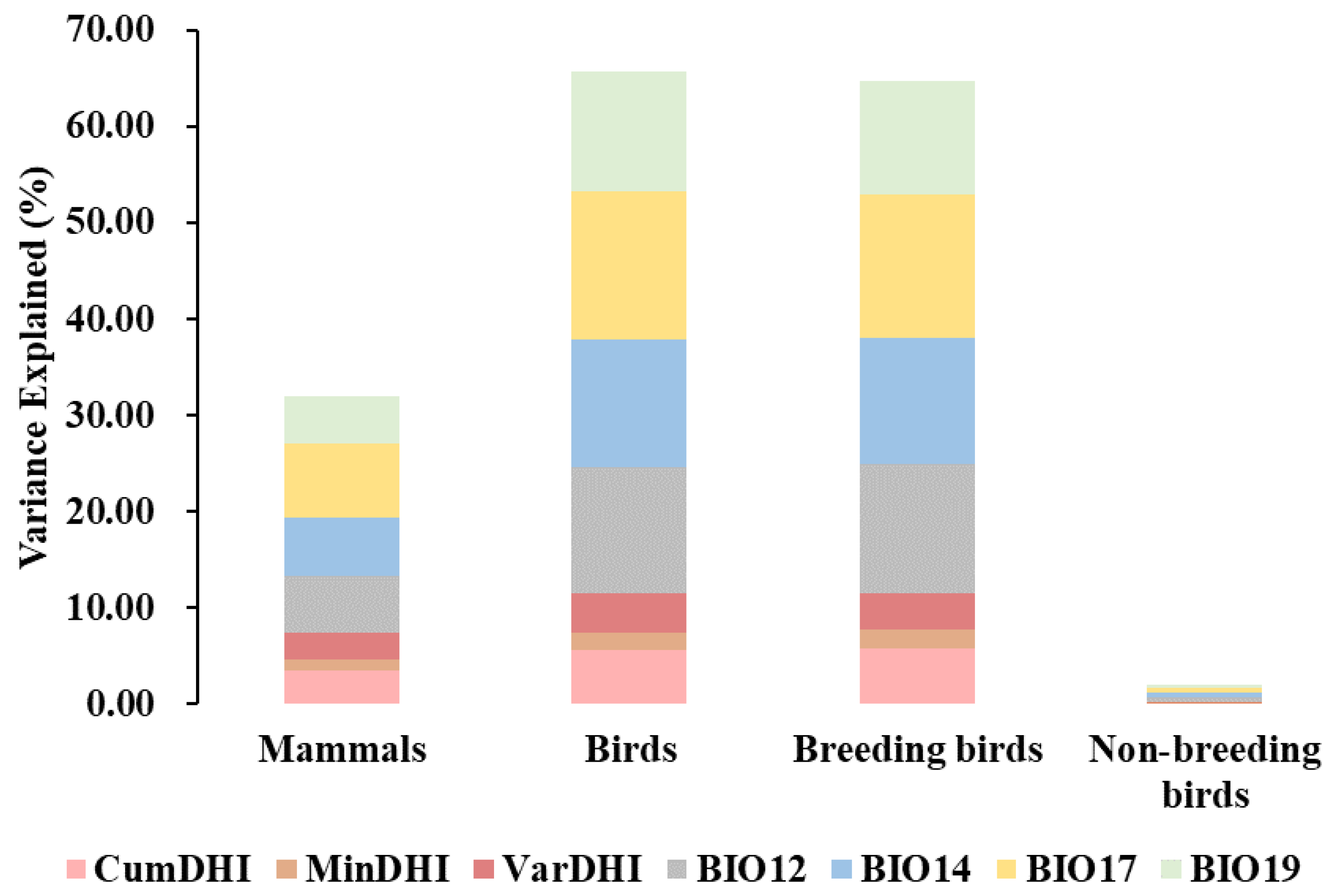
3.4. The Combined Effect of the Productivity Hypothesis and Water–Energy Dynamics Hypothesis on Species Richness

The productivity hypothesis and water–energy dynamics hypothesis explained the distribution of species richness in the Kunlun–Pamir Plateau from a different aspect (Figure 8). Combining the two hypotheses could help to fully understand the species richness distribution in the Kunlun–Pamir Plateau. Our analysis of the combination of two hypotheses demonstrated that the explanatory power of the multiple regression models on species richness improved when compared to the single regression models based on each hypothesis separately, except for the non-breeding birds (Table 5). In particular, the model improved from 0.24 to 0.32 for mammals, 0.54 to 0.66 for birds and 0.54 to 0.65 for breeding birds. The multiple regression model’s hierarchical partitioning analysis revealed that all seven influences played a key role when explaining the overall variability in species richness. BIO17 identified the most significant species richness regressions for the mammals, birds and breeding birds, while BIO12 was the most important for the non-breeding birds. The minimum DHI based on the FPAR was the least crucial for all models. The regression model for birds mainly justified the species richness variation among the four taxa (Figure 9).

4. Discussion

4.1. The Application of the Productivity Hypothesis

Revealing the species richness patterns is essential for the biodiversity, especially for the conservation of endangered species in the Kunlun–Pamir Plateau area. However, only a few studies have focused on the biodiversity in this region. We constructed five DHIs based on the MODIS NDVI, EVI, FPAR, LAI and GPP data, and we assessed their performance in the species richness models on the Kunlun–Pamir Plateau. The findings revealed that the three DHIs (CumDHI, MinDHI and VarDHI) correlated weakly with the species richness, suggesting that the concept of the productivity hypothesis does not apply well to the desert plateau locations. Among these four taxa, the explanatory power of the FPAR-based multiple regression models (for DHIs) was revealed to be weaker when compared to the application of the DHIs in other regions (Table 3). However, the correlations appeared the most vital for birds and least worthwhile for the non-breeding birds. Our findings were consistent with the results of other studies [22]. According to earlier research [27,28], the FPAR captures more subtle changes in the grassland photosynthetic activity; therefore, derived DHIs perform best regarding the grassland breeding species, and our results support this. In addition, contrary to other studies, the land cover in the Kunlun–Pamir Plateau region is dominated by bare land and grasslands, in which the species richness correlated positively with the VarDHI based on the FPAR, making the results more reasonable. However, the DHIs based on the FPAR in this study area did not indicate an obvious spatial pattern relative to the large-scale studies. Moreover, the correlations between the species richness and the DHIs based on the FPAR were rather small, demonstrating that the applicability of the DHIs based on the FPAR still needs further testing in relatively sparse vegetated mountainous areas.

4.2. The Application of the Water–Energy Dynamic Hypothesis

Understanding the factors affecting the species’ distribution and the diversity patterns is essential to conserve the regional species richness [11,42]. The water–energy dynamics hypothesis interpreted the main influencing factors affecting the species in the Kunlun–Pamir Plateau region regarding energy and moisture. The results showed that the moisture significantly influenced the species richness more than energy in the Kunlun–Pamir Plateau area. The correlations between the variables related to the moisture factor, and the mammals, birds, breeding birds and non-breeding birds were 0.29, 0.61 and 0.60, respectively (Table 4). The moisture had a relatively important influence on the Kunlun–Pamir Plateau area, which confirmed O’Brien’s conclusion regarding the main influencing factors on the species richness distribution patterns in arid regions [43]. The water–energy dynamics hypothesis was applicable to explain the species richness distribution patterns. Moisture is the main factor affecting the species richness in the Kunlun–Pamir Plateau region due to the continental alpine climate with sufficient sunshine and low rainfall [44]. As the plateau continues to warm, the snowpack will decrease or fluctuate, which may significantly impact the species richness [45]. Therefore, in the Kunlun–Pamir Plateau region, further research on how climate change effects biodiversity will be essential.

4.3. Limitations

In this study, we investigated the factors that affect the species richness in the Kunlun–Pamir Plateau region only from the view of two perspectives: the productivity hypothesis and the water–energy dynamics hypothesis. However, an increasing number of studies have already shown that the mechanisms underlying the geographic patterns of species richness are complex and cannot be explained by only one hypothesis [9,11]. Thus, the productivity and water–energy dynamics hypotheses were joined in this work, and various regression models were employed to improve the model’s interpretation of species richness. However, the species richness change was also influenced by land use change, invasive alien species and other elements [2,46,47,48,49]. More factors still need to be considered among the factors impacting the species richness patterns, such as the topographic factors [50], human disturbance [47] and spatial correlation [8,51]. Future studies should include more causal factors for species richness in order to reveal the mechanism that maintains the species richness distribution pattern of the Kunlun–Pamir Plateau more thoroughly.

5. Conclusions

We analyzed the species richness pattern in the Kunlun–Pamir Plateau region, taking into account both the productivity hypothesis and the water–energy dynamics hypothesis.
From the aspect of the productivity hypothesis, we investigated the correlation between the dynamic habitat indices (DHIs) and the species richness in the Kunlun–Pamir Plateau region. The calculated DHIs by means of five MODIS products correlated less with the mammal, bird, breeding bird and non-breeding bird richness in the Kunlun–Pamir Plateau region. The DHIs based on the FPAR data correlated slightly higher with the mammal, bird, breeding bird and non-breeding bird richness than those based on the other four MODIS product DHIs. Although the cumulative DHIs based on the FPAR conformed more with the richness of the four taxa species compared to the variation based on the FPAR and minimum DHIs based on the FPAR, the multiple regression models for the three variables associated better with the richness of the four species. However, the DHI based on the FPAR correlation coefficients with an abundance of mammals, birds, breeding birds and non-breeding birds were still low, namely 0.24, 0.25, 0.24 and 0.01, respectively. The birds regression model clarified most of the variations in species richness during the four taxa.
Regarding the water–energy dynamics hypothesis, the precipitation-related climatic factors dominate the distribution of species richness on the Kunlun–Pamir Plateau; among those, BIO12 had the highest correlations with mammals, birds, breeding birds and non-breeding birds, amounting to 0.24, 0.54, 0.54 and 0.02, respectively, followed by BIO17, -19 and -14. Multiple linear regression models (based on four climate factors) raised the correlations between these factors with the mammals, birds, breeding birds and non-breeding birds (to 0.29). Furthermore, we noticed that the correlation between the species richness and the climatic factors was noticeably higher in the Kunlun–Pamir Plateau than the MODIS-based DHIs. The correlations between the DHIs based on the FPAR and the climate factors increased to 0.32, 0.66, 0.65 and 0.02, respectively, for the multivariate linear regression models. The regression model for birds also explained the majority of the variations in species richness for the four taxa. The water–energy dynamic hypothesis was more appropriate to the Kunlun–Pamir Plateau region.
In general, by examining the DHIs and the species richness in specific areas, we suggest a reconstruction of the DHIs appropriate for the region, especially for locations with relatively small spatial scales. In the context of climate change, our results once again highlight the significance of monitoring climate fluctuations in the Kunlun–Pamir region for biodiversity conservation. This will make it easier to evaluate the spatial distribution of species richness and provide an accurate assessment of that distribution.

Supplementary Materials

The following supporting information can be downloaded at: https://www.mdpi.com/article/10.3390/rs14246187/s1: Table S1: Coefficient of determination between the individual EVI -based DHIs of the four main taxa; Table S2: Coefficient of determination between the individual GPP -based DHIs of the four main taxa; Table S3: Coefficient of determination between the individual LAI -based DHIs of the four main taxa; Table S4: Coefficient of determination between the individual NDVI -based DHIs of the four main taxa; Table S5: Coefficient of determination between the individual NDVI -based DHIs of the four main taxa.

Author Contributions

Conceptualization, X.H. and A.B.; methodology, X.H. and A.B.; data curation and software, J.Z.; validation, X.H. and T.Y.; formal analysis, X.H. and G.Z; resources, X.H.; data curation, X.H.; writing—original draft preparation, X.H. and G.Z.; writing—review and editing, A.B., Y.Y., T.W., V.N., P.D.M. and T.V.d.V.; visualization, X.H.; supervision, A.B.; project administration, A.B. and funding acquisition, A.B. All authors have read and agreed to the published version of the manuscript.

Funding

This research was supported by the Strategic Priority Research Program of the Chinese Academy of Sciences (Grant No. XDA20030101), the Qinghai Province Kunlun talents—leading talents project (2020-LCJ-02).

Conflicts of Interest

The authors declare no conflict of interest.

References

  1. Gotelli, N.J.; Colwell, R.K. Quantifying biodiversity: Procedures and pitfalls in the measurement and comparison of species richness. Ecol. Lett. 2001, 4, 379–391. [Google Scholar] [CrossRef] [Green Version]
  2. D’Antraccoli, M.; Roma-Marzio, F.; Carta, A.; Landi, S.; Bedini, G.; Chiarucci, A.; Peruzzi, L. Drivers of floristic richness in the Mediterranean: A case study from Tuscany. Biodivers. Conserv. 2019, 28, 1411–1429. [Google Scholar] [CrossRef]
  3. Balmford, A.; Green, R.E.; Jenkins, M. Measuring the changing state of nature. Trends Ecol. Evol. 2003, 18, 326–330. [Google Scholar] [CrossRef]
  4. Butchart, S.H.M.; Walpole, M.; Collen, B.; van Strien, A.; Scharlemann, J.P.W.; Almond, R.E.A.; Baillie, J.E.M.; Bomhard, B.; Brown, C.; Bruno, J.; et al. Global Biodiversity: Indicators of Recent Declines. Science 2010, 328, 1164–1168. [Google Scholar] [CrossRef] [PubMed]
  5. Brown, J.H. Two Decades of Homage to Santa Rosalia: Toward a General Theory of Diversity. Am. Zool. 1981, 21, 877–888. [Google Scholar] [CrossRef] [Green Version]
  6. Wright, D.H. Species-Energy Theory: An Extension of Species-Area Theory. Oikos 1983, 41, 496. [Google Scholar] [CrossRef] [Green Version]
  7. O’Brien, E.M. Climatic Gradients in Woody Plant Species Richness: Towards an Explanation Based on an Analysis of Southern Africa’s Woody Flora. J. Biogeogr. 1993, 20, 181–198. [Google Scholar] [CrossRef]
  8. Hawkins, B.A.; Porter, E.E. Water-energy balance and the geographic pattern of speciesrichness of western Palearctic butterflies. Ecol. Entomol. 2010, 28, 678–686. [Google Scholar] [CrossRef] [Green Version]
  9. Currie, D.J. Energy and large-scale patterns of animal- andplant-species richness. Am. Nat. 1991, 137, 27–49. [Google Scholar] [CrossRef]
  10. Turner, J.R. Explaining the global biodiversity gradient: Energy, area, history and natural selection. Basic Appl. Ecol. 2004, 5, 435–448. [Google Scholar] [CrossRef]
  11. Hawkins, B.A.; Field, R.; Cornell, H.V.; Currie, D.J.; Guégan, J.; Kaufman, D.M.; Kerr, J.T.; Mittelbach, G.G.; Oberdorff, T.; O’Brien, E.M.; et al. Energy, water, and broad-scale geographic patternsof species richness. Ecology 2003, 84, 3105–3117. [Google Scholar] [CrossRef] [Green Version]
  12. Gillooly, J.F.; Brown, J.H.; West, G.B.; Savage, V.M.; Charnov, E.L. Effects of size and temperature on metabolic rate. Science 2001, 293, 2248–2251. [Google Scholar] [CrossRef] [PubMed] [Green Version]
  13. Allen, A.P.; Brown, J.H.; Gillooly, J.F. Global biodiversity, biochemical kinetics, and the energetic-equivalence rule. Science 2002, 297, 1545–1548. [Google Scholar] [CrossRef] [PubMed]
  14. Brown, J.H.; Gillooly, J.F.; Allen, A.P.; Savage, V.M.; West, G.B. Toward a metabolic theory of ecology. Ecology 2004, 85, 1771–1789. [Google Scholar] [CrossRef]
  15. Gaston, K.J. Global patterns in biodiversity. Nature 2000, 405, 220–227. [Google Scholar] [CrossRef]
  16. Evans, K.L.; James, N.; Gaston, K.J. Abundance, species richness and energy availability in the North American avifauna. Glob. Ecol. Biogeogr. 2006, 15, 372–385. [Google Scholar] [CrossRef]
  17. O’Brien, E.M. Biological relativity to water?energy dynamics. J. Biogeogr. 2010, 33, 1868–1888. [Google Scholar] [CrossRef]
  18. Qian, H.; Wang, X.; Wang, S.; Li, Y. Environmental determinants of amphibian and reptile species richness in China. Ecography 2007, 30, 471–482. [Google Scholar] [CrossRef]
  19. Huang, C.-y. Using Geographical Variation of Water and Energy to Explainthe Spatial Distribution Patterns of Pteridophyta of China; Shanxi University: Taiyuan, China, 2018. [Google Scholar]
  20. Hurlbert, A.H.; Haskell, J.P. The effect of energy and seasonality on avian species richness and community composition. Am. Nat. 2003, 161, 83–97. [Google Scholar] [CrossRef]
  21. St-Louis, V.; Pidgeon, A.M.; Clayton, M.K.; Locke, B.A.; Bash, D.; Radeloff, V.C. Satellite image texture and a vegetation index predict avian biodiversity in the Chihuahuan Desert of New Mexico. Ecography 2009, 32, 468–480. [Google Scholar] [CrossRef]
  22. Hobi, M.L.; Dubinin, M.; Graham, C.H.; Coops, N.C.; Clayton, M.K.; Pidgeon, A.M.; Radeloff, V.C. A comparison of Dynamic Habitat Indices derived from different MODIS products as predictors of avian species richness. Remote Sens. Environ. 2017, 195, 142–152. [Google Scholar] [CrossRef]
  23. Scholes, R.J.; Walters, M.; Turak, E.; Saarenmaa, H.; Heip, C.H.; Tuama, É.Ó.; Faith, D.P.; Mooney, H.A.; Ferrier, S.; Jongman, R.H.; et al. Building a global observing system for biodiversity. Curr. Opin. Environ. Sustain. 2012, 4, 139–146. [Google Scholar] [CrossRef]
  24. Pereira, H.M.; Ferrier, S.; Walters, M.; Geller, G.N.; Jongman, R.H.G.; Scholes, R.J.; Bruford, M.W.; Brummitt, N.; Butchart, S.H.M.; Cardoso, A.C.; et al. Essential Biodiversity Variables. Science 2013, 339, 277–278. [Google Scholar] [CrossRef] [PubMed] [Green Version]
  25. Wang, K.; Franklin, S.E.; Guo, X.; He, Y.; McDermid, G.J. Problems in remote sensing of landscapes and habitats. Prog. Phys. Geogr. Earth Environ. 2009, 33, 747–768. [Google Scholar] [CrossRef] [Green Version]
  26. Radeloff, V.; Dubinin, M.; Coops, N.; Allen, A.; Brooks, T.; Clayton, M.; Costa, G.; Graham, C.; Helmers, D.; Ives, A.; et al. The Dynamic Habitat Indices (DHIs) from MODIS and global biodiversity. Remote Sens. Environ. 2019, 222, 204–214. [Google Scholar] [CrossRef]
  27. Coops, N.C.; Waring, R.H.; Wulder, M.A.; Pidgeon, A.M.; Radeloff, V.C. Bird diversity: A predictable function of satellite-derived estimates of seasonal variation in canopy light absorbance across the United States. J. Biogeogr. 2009, 36, 905–918. [Google Scholar] [CrossRef]
  28. Coops, N.C.; Wulder, M.; Iwanicka, D. Demonstration of a satellite-based index to monitor habitat at continental-scales. Ecol. Indic. 2009, 9, 948–958. [Google Scholar] [CrossRef]
  29. Andrew, M.E.; Wulder, M.A.; Coops, N.C.; Baillargeon, G. Beta-diversity gradients of butterflies along productivity axes. Glob. Ecol. Biogeogr. 2012, 21, 352–364. [Google Scholar] [CrossRef] [Green Version]
  30. Michaud, J.-S.; Coops, N.C.; Andrew, M.E.; Wulder, M.A.; Brown, G.S.; Rickbeil, G.J. Estimating moose (Alces alces ) occurrence and abundance from remotely derived environmental indicators. Remote Sens. Environ. 2014, 152, 190–201. [Google Scholar] [CrossRef]
  31. Zhang, C.; Cai, D.; Guo, S.; Guan, Y.; Fraedrich, K.; Nie, Y.; Liu, X.; Bian, X. Spatial-Temporal Dynamics of China’s Terrestrial Biodiversity: A Dynamic Habitat Index Diagnostic. Remote Sens. 2016, 8, 227. [Google Scholar] [CrossRef]
  32. Razenkova, E.; Radeloff, V.C.; Dubinin, M.; Bragina, E.V.; Allen, A.M.; Clayton, M.K.; Pidgeon, A.M.; Baskin, L.M.; Coops, N.C.; Hobi, M. Vegetation productivity summarized by the Dynamic Habitat Indices explains broad-scale patterns of moose abundance across Russia. Sci. Rep. 2020, 10, 836. [Google Scholar] [CrossRef] [PubMed] [Green Version]
  33. Zhang, H.; Li, Z.; Zhou, P. Mass balance reconstruction for Shiyi Glacier in the Qilian Mountains, Northeastern Tibetan Plateau, and its climatic drivers. Clim. Dyn. 2020, 56, 969–984. [Google Scholar] [CrossRef]
  34. Jenkins, C.N.; Pimm, S.L.; Joppa, L.N. Global patterns of terrestrial vertebrate diversity and conservation. Proc. Natl. Acad. Sci. USA 2013, 110, E2602–E2610. [Google Scholar] [CrossRef] [PubMed] [Green Version]
  35. Pimm, S.L.; Jenkins, C.N.; Abell, R.; Brooks, T.M.; Gittleman, J.L.; Joppa, L.N.; Raven, P.H.; Roberts, C.M.; Sexton, J.O. The biodiversity of species and their rates of extinction, distribution, and protection. Science 2014, 344, 1246752. [Google Scholar] [CrossRef] [PubMed]
  36. Jenkins, C.N.; Van Houtan, K.S. Global and regional priorities for marine biodiversity protection. Biol. Conserv. 2016, 204, 333–339. [Google Scholar] [CrossRef]
  37. IUCN. IUCN Red List of Threatened Species; Version 2018-1. Available online: http://www.iucnredlist.org (accessed on 7 August 2022).
  38. BirdLife International and Handbook of the Birds of the World. Bird Species Distribution Maps of the World. Version 7.0. 2018. Available online: http://datazone.birdlife.org/species/requestdis (accessed on 7 August 2022).
  39. Zhang Chunyan, G.S.; Yanning, G.; Danlu, C.; Lei, Y.W.W.; Han, X. A global dataset of monthly maximum fractions of photosyntheticallyactive radiation of the continents (2001–2010). China Sci. Data 2017, 2, 52–61. [Google Scholar]
  40. Coops, N.C.; Wulder, M.A.; Duro, D.C.; Han, T.; Berry, S. The development of a Canadian dynamic habitat index using multi–temporal satellite estimates of canopy light absorbance. Ecol. Indic. 2008, 8, 754–766. [Google Scholar] [CrossRef]
  41. Mac Nally, R.; Walsh, C.J. Hierarchical partitioning public-domain software. Biodivers. Conserv. 2004, 13, 659. [Google Scholar] [CrossRef]
  42. Li, L.; Wang, Z.; Zerbe, S.; Abdusalih, N.; Tang, Z.; Ma, M.; Yin, L.; Mohammat, A.; Han, W.; Fang, J. Species richness patterns and water-energy dynamics in the drylands of northwest China. PLoS ONE 2013, 8, e66450. [Google Scholar] [CrossRef] [PubMed]
  43. O’Brien, E.M. Water-energy dynamics, climate, and prediction of woody plant species richness: An interim general model. J. Biogeogr. 1998, 25, 379–398. [Google Scholar] [CrossRef]
  44. Dai Kui, S. Estimation and impact factor of wild ungulates population in west Kunlun mountain area. J. Green Sci. Technol. 2012, 4, 3–5. [Google Scholar]
  45. Sutherland, W.J.; Butchart, S.H.M.; Connor, B.; Culshaw, C.; Dicks, L.V.; Dinsdale, J.; Doran, H.; Entwistle, A.C.; Fleishman, E.; Gibbons, D.W. A 2018 Horizon Scan of Emerging Issues for Global Conservation and Biological Diversity. Trends Ecol. Evol. 2018, 33, 47–58. [Google Scholar] [CrossRef]
  46. Ferrer-Castán, D.; Morales-Barbero, J.; Vetaas, O.R. Water-energy dynamics, habitat heterogeneity, history, and broad-scale patterns of mammal diversity. Acta Oecologica 2016, 77, 176–186. [Google Scholar] [CrossRef]
  47. Newbold, T.; Hudson, L.N.; Hill, S.L.L.; Contu, S.; Lysenko, I.; Senior, R.A.; Börger, L.; Bennett, D.J.; Choimes, A.; Collen, B.; et al. Global effects of land use on local terrestrial biodiversity. Nature 2015, 520, 45. [Google Scholar] [CrossRef] [Green Version]
  48. Cahill, A.E.; Aiello-Lammens, M.; Fisher-Reid, M.C.; Hua, X.; Karanewsky, C.J.; Ryu, H.Y.; Sbeglia, G.C.; Spagnolo, F.; Waldron, J.B.; Warsi, O.; et al. How does climate change cause extinction? Proc. R. Soc. B Boil. Sci. 2013, 280, 20121890. [Google Scholar] [CrossRef]
  49. Wang, X.; Liu, S.; Ding, Y.; Guo, W.; Jiang, Z.; Lin, J.; Han, Y. An approach for estimating the breach probabilities of moraine-dammed lakes in the Chinese Himalayas using remote-sensing data. Nat. Hazards Earth Syst. Sci. 2012, 12, 3109–3122. [Google Scholar] [CrossRef] [Green Version]
  50. Larsen, L.G.; Harvey, J. Modeling of hydroecological feedbacks predicts distinct classes of landscape pattern, process, and restoration potential in shallow aquatic ecosystems. Geomorphology 2010, 126, 279–296. [Google Scholar] [CrossRef]
  51. Chen, S.; Mao, L.; Zhang, J.; Zhou, K.; Gao, J. Environmental determinants of geographic butterflyrichness pattern in eastern China. Biodivers. Conserv. 2014, 23, 1453–1467. [Google Scholar] [CrossRef]
Figure 1. The spatial patterns of three DHIs derived from (ac) the NDVI, (df) LAI, (gi) GPP, (jl) FPAR and (mo) EVI.
Remotesensing 14 06187 g001
Figure 2. Spearman rank correlations and scatter plots among the three DHIs derived from the five MODIS products. It represents a correlation matrix for cum–min–var with scatter plots on one side of the diagonal and correlations on the other side. Significant relations: *** p < 0.001.
Remotesensing 14 06187 g002
Figure 3. Spearman rank correlations and scatter plots among the three DHIs derived from various MODIS products. Significant relations: *** p < 0.001.
Remotesensing 14 06187 g003
Figure 4. Pairs of the Spearman correlations of all MODIS FPAR-based DHIs versus the environmental variables grouped by (a) DHIs and temperature variables from Bioclim and (b) DHIs and precipitation values from Bioclim. Significant relations: * p < 0.05; ** p < 0.01; *** p < 0.001.
Remotesensing 14 06187 g004aRemotesensing 14 06187 g004b
Figure 5. Distribution of species richness of (a) mammals, (b) birds, (c) breeding birds and (d) non-breeding birds.
Remotesensing 14 06187 g005
Figure 6. The relative importance of the three FPAR-based DHIs to the four main taxa.
Remotesensing 14 06187 g006
Figure 7. The relative importance of the four Bioclim variables and the four main taxa.
Remotesensing 14 06187 g007
Figure 8. Pairs of the Spearman correlations of all MODIS FPAR-based DHIs and the four Bioclim variables (BIO12, BIO14, BIO17 and BIO19) versus the species richness of the four taxa (mammals, birds, breeding birds and non-breeding birds). Significant relations: *** p < 0.001.
Remotesensing 14 06187 g008
Figure 9. The relative importance of (the) three FPAR-based DHIs, as well as four Bioclim variables to the four taxa.
Remotesensing 14 06187 g009
Table 1. MODIS products used to calculate the DHIs.
IndexNamePlatformTemporal Resolution (Day)Spatial Resolution
(m)
NDVIMOD13A1Terra16500
EVIMOD13A1Terra16500
FPARMOD15A2HTerra8500
LAIMOD15A2HTerra8500
GPPMOD17A2HGFTerra8500
Table 2. Nineteen Worldclim Bioclim variables used to test the water–energy dynamics hypothesis.
VariablesDescription
Energy factorBIO1Annual Mean Temperature
BIO2Mean Diurnal Range
BIO3Isothermality
BIO4Temperature Seasonality
BIO5Max Temperature of Warmest Month
BIO6Min Temperature of Coldest Month
BIO7Temperature Annual Range
BIO8Mean Temperature of Wettest Quarter
BIO9Mean Temperature of Driest Quarter
BIO10Mean Temperature of Warmest Quarter
BIO11Mean Temperature of Coldest Quarter
Water factorsBIO12Annual Precipitation
BIO13Precipitation of Wettest Month
BIO14Precipitation of Driest Month
BIO15Precipitation Seasonality
BIO16Precipitation of Wettest Quarter
BIO17Precipitation of Driest Quarter
BIO18Precipitation of Warmest Quarter
BIO19Precipitation of Coldest Quarter
Table 3. Coefficient of determination between the individual FPAR-based DHIs of the four main taxa. Significant relations: ** p < 0.01; *** p < 0.001.
Cumulative DHI
R2 Adj
RMSEMinimum DHI R2 AdjRMSEVariation DHI R2 AdjRMSEAll DHIs R2 AdjRMSE
Mammals0.12 ***7.030.03 ***7.380.12 ***7.040.14 ***6.98
Birds0.20 ***37.100.04 ***40.590.19 ***37.420.25 ***36.73
Breeding birds0.20 ***34.950.05 ***38.170.18 ***35.400.24 ***34.66
Non-breeding birds0.00 ***18.970.00 **19.010.00 ***18.980.01 ***18.97
Table 4. Coefficient of determination between the Bioclim variables (BIO12, BIO14, BIO17 and BIO19) and four main taxa. Significant relations: * p < 0.05; *** p < 0.001.
BIO12
R2 Adj
RMSEBIO14
R2 Adj
RMSEBIO17
R2 Adj
RMSEBIO19
R2 Adj
RMSEThe Four
BIOs R2 Adj
RMSE
Mammals0.24 ***6.540.20 ***6.700.23 ***6.590.21 ***6.650.29 ***6.32
Birds0.54 ***28.120.49 ***29.600.53 ***28.480.52 ***28.910.61 ***25.82
Breeding birds0.54 ***26.550.49 ***27.920.52 ***27.070.50 ***18.850.60 ***24.69
Non-breeding birds0.02 ***18.840.02 ***18.860.02 ***18.850.02 *18.850.02 ***18.82
Table 5. Coefficient of determination between the four Bioclim variables (BIO12, BIO14, BIO17 and BIO19), as well as the FPAR-based DHIs to the three significant relations: *** p < 0.001.
Four BIOs and Three FPAR-Based DHIs
R2 Adj
RMSE
Mammals0.32 ***6.18
Birds0.66 ***24.34
Breeding birds0.65 ***23.28
Non-breeding birds0.02 ***18.82
Publisher’s Note: MDPI stays neutral with regard to jurisdictional claims in published maps and institutional affiliations.

