Article

LightFGCNet: A Lightweight and Focusing on Global Context Information Semantic Segmentation Network for Remote Sensing Imagery

1
Institute of Applied Optimization, School of Artificial Intelligence and Big Data, Hefei University, Hefei 230601, China
2
Department of Big Data and Information Engineering, School of Artificial Intelligence and Big Data, Hefei University, Hefei 230601, China
*
Author to whom correspondence should be addressed.
Remote Sens. 2022, 14(24), 6193; https://doi.org/10.3390/rs14246193
Submission received: 21 October 2022 / Revised: 25 November 2022 / Accepted: 3 December 2022 / Published: 7 December 2022

Abstract

:
Convolutional neural networks have attracted much attention for their use in the semantic segmentation of remote sensing imagery. The effectiveness of semantic segmentation of remote sensing images is significantly influenced by contextual information extraction. The traditional convolutional neural network is constrained by the size of the convolution kernel and mainly concentrates on local contextual information. We suggest a new lightweight global context semantic segmentation network, LightFGCNet, to fully utilize the global context data and to further reduce the model parameters. It uses an encoder–decoder architecture and gradually combines feature information from adjacent encoder blocks during the decoding upsampling stage, allowing the network to better extract global context information. Considering that the frequent merging of feature information produces a significant quantity of redundant noise, we build a unique and lightweight parallel channel spatial attention module (PCSAM) for a few critical contextual features. Additionally, we design a multi-scale fusion module (MSFM) to acquire multi-scale feature target information. We conduct comprehensive experiments on the two well-known datasets ISPRS Vaihingen and WHU Building. The findings demonstrate that our suggested strategy can efficiently decrease the number of parameters. Separately, the number of parameters and FLOPs are 3.12 M and 23.5 G, respectively, and the mIoU and IoU of our model on the two datasets are 70.45% and 89.87%, respectively, which is significantly better than what the conventional convolutional neural networks for semantic segmentation can deliver.

Graphical Abstract

1. Introduction

In contrast to natural images, remote sensing images are taken from the air using satellites or aircraft and are not constrained by geography or spatial location. As a result, they offer remarkable benefits in areas such as land planning, disaster monitoring, vegetation monitoring, and urban management [1].
Convolution neural networks (CNNs) with their end-to-end advantages have accelerated the development of semantic segmentation since the fully convolutional network (FCN) was first introduced [2]. The encoder–decoder architecture is used in the majority of CNNs-based networks. Although first used to segment medical images, Unet [3], a standard u-shaped encoder–decoder network, is a viable option for semantic segmentation in remote sensing. Given that it uses skip connections to link the encoder and decoder, it can fully utilize the contextual information taken at various stages to get more edge details. Atrous convolution with diverse dilation rates is implemented in the DeepLab series [4,5,6,7], which has a better segmentation effect on multi-scale targets. VIT [8] serializes the image to enable it to comprehend the image from a global perspective, in contrast to CNNs-based networks, which are biased to focus on local contextual information. Efficient-T [9] is intended to be lightweight and performs well in the semantic segmentation of remote sensing images because training VIT involves extensive computational resources.
With the rapid development of aerospace and sensor technologies, researchers can easily and quickly obtain high-resolution orthorectified aerial images. This increases the number of multi-scale and multi-class objects in the remote sensing image dataset, bringing the collected images closer to the actual scene. Consequently, the semantic segmentation of remote sensing images faces the issue of an imbalanced intra-class scale and inter-class distribution. As shown in Figure 1, five various scales of objects are presented in the cropped high-resolution remote sensing image. From the whole dataset, the distribution of large-scale objects, such as buildings and impervious surfaces, accounts for the majority, while there are only a few small-scale targets, such as cars and backgrounds. In addition, the area defined by the red dashed line in Figure 1 reveals that the majority of the target borders in the remote sensing images are irregular, making it extremely challenging to identify the image boundary features. In remote sensing images, instances of the same class have situations in which features such as color, shape, and texture vary greatly, which leads to the network’s misclassification.
The semantic segmentation of remote sensing images presents unique challenges due to the complexity of the segmentation context and the similarity of attribute traits among objects. Therefore, the network must pay close attention to the global context and boundary details as it extracts features. The downsampling procedure of max-pooling can be used to transform high-resolution feature maps into low-resolution feature maps and is employed to extract semantic information to lower the computational cost and extend the receptive field of CNNs. However, this can lead to the loss of some spatial information. An increasingly popular method for dealing with this issue is to use skip connections in a higher layer to fuse with the feature information from a lower layer. CGNet [10] combines contextual data from earlier stages at each successive level but ignores a large amount of noise that might be generated after frequent fusion. HRCNet [11] uses the high-resolution and low-resolution branch fusion of HRNet [12] to enhance the edge accuracy. Furthermore, remote sensing images store more information than natural images, yet some redundant information may decrease the segmentation effectiveness of the network. The final recovered features will likewise have a lot of noise after many convolution steps. By assigning different weights to the feature map dimensions, the attention mechanism can help mitigate this effect of noise on segmentation and bring focus to the crucial details [13]. Channel attention, for instance, can produce an attention mask on the channel dimension to identify the key channels. At the feature map level of each channel, spatial attention is employed to filter out noise and emphasize the pixels that need to be prioritized.
Based on the research mentioned earlier, our suggested approach iteratively fuses feature information derived from neighboring stages of the encoder to improve the global contextual knowledge of the network. We introduce new channel and spatial attention components to maintain the payoff dimensions via mean and median operations. Then, the crucial channels and pixels extracted based on trainable weights are chosen. As a novel approach to multi-dimensional screening, we construct a channel spatial attention module by coupling channel attention with spatial attention in parallel. Compared to other attention modules that use a single attention mechanism, our attention module is able to select key information independently for both space and channel. At the same time, we choose a combination of median and mean to retain features, which can retain more balanced feature information than other attentional methods. In addition, for multi-scale targets, most of the multi-scale features are currently extracted by parallel atrous convolutions. We add a multi-scale fusion module in the middle of the decoder and use a serial concatenation of atrous convolution and standard convolution with different atrous rates. It is able to capture more semantic information while reducing the level of downsampling and obtaining a larger receptive field. The following is a brief overview of our most important contributions:
We propose the lightweight semantic segmentation network, LightFGCNet, which prioritizes global contextual information by fusing feature information of varying resolutions multiple times.
We develop a simple and effective parallel channel spatial attention module (PCSAM), which is a redesigned version of the previously existing channel attention and spatial attention modules that now work together in parallel to reduce noise from multiple fusions.
Inspired by the atrous spatial convolution pooling pyramid, we construct a multi-scale fusion module (MSFM), geared towards the needs of the premise of fewer parameters, to extract more multi-scale information and increase context information.

2. Related Work

2.1. Contextual Information

The accuracy in the semantic segmentation of remote sensing images can be improved by gathering additional contextual information. Chen et al. [14] describe the significance of image context in boosting accuracy. Expanding the receptive field of the kernel is one method of capturing contextual information. By combining the characteristics of the pooling layers, the earliest FCN can already acquire contextual information during upsampling, although this method of increasing the receptive field at the expense of some spatial details is not optimal. The atrous spatial pyramid pooling (ASPP) is a novel module in DeepLab V2 developed to collect multi-scale contextual data. Because of the sparse sampling and the limited number of pixels used for calculation, the atrous convolution results in a significant loss of semantic association among adjacent pixels. DenseASPP [15] adapts the concept of dense connection from DenseNet [16] to ASPP, expanding the receptive field by increasing the number of sample points at the expense of processing resources.
Another example is HRNet, which maintains the integrity of the high-resolution branches of the network while empowering its low-resolution branches to exchange context via a combination of features. To record the context of the feature map, SRANet [17] creates a semantic relationship aware module (SRAM) based on a self-attention mechanism and makes a separable space convergence pyramid (SSCP) to collect multi-scale context information. Through bidirectional information propagation, PSANet [18] can adaptively learn context on a point-wise basis. SPN [19] builds a linear propagation model of rows and columns to record dense and global pairwise associations in images. Models for deep representation learning that rely on graph message forwarding are also available. DGMN [20] dynamically predicts filtering weights and a relation matrix based on node conditions to disseminate background context among feature nodes. MSDAE [21] is based on a multi-scale denoising autoencoder model that combines information from multiple-scale representations of reconstructed spectral features.
In this research, we create a simple network design. Additionally, using skip connections, the context data from the previous encoder stage is continuously fused in the decoder to capture more global contextual information. We also include a multi-scale fusion module for extracting multi-scale contextual content in the decoder.

2.2. Attention Mechanism

It is the primary function of the attention mechanism to give greater emphasis to those components that have been identified as requiring special care. Channel attention adaptively modifies the channel dimension weights to direct the attention of the network to the important objects. In order to improve feature representation, the earliest squeeze-excitation (SE) module first introduced in SENet [22] is used to capture correlations between channel dimensions. The issues that exist in both the squeeze and excitation parts of the SE block are mitigated by subsequent channel attention modules. For example, the problem that the global average pooling in the squeeze of the SE block is too simplistic to obtain global information is addressed in GsoPNet [23] as follows. In the squeeze phase, the number of channels is decreased via 1 × 1 convolution, a covariance matrix is computed for each set of channels to determine their correlation. Finally, the covariance matrix is normalized row by row. The connection between channels in ECANet [24] is calculated using a 1D convolution. The k-nearest neighbor approach is used to regulate the complexity of the model, which only takes into account the interaction between neighboring channels. FcaNet [25] proved that the global average pooling (GAP) is a special case of the discrete cosine transform (DCT), and based on this, the GAP was extended to the frequency domain, thus proposing a multispectral channel attention framework.
The ability to focus on key locations of the feature maps can be thought of as an adaptive mechanism of spatial attention. In RAM [26], a recurrent neural network (RNN) and reinforcement learning are used to train the network to recognize which features merit its focus. RAM is the pioneering application of RNN for focusing on computer vision tasks. Sub-networks are used in STN [27] to define the predicted regions of interest. GENet [28] refers to those who implicitly predict soft masks using sub-networks in order to identify key regions. Thanks to its lightweight and simple features, the attention module can be plug-and-play into most networks. Channel attention and spatial attention are often used to fuse and enhance multi-scale feature information in building extraction in remote sensing field. MAP-Net [29] innovatively uses parallel multi-path networks to extract multi-scale information and to further improve the accuracy of building boundaries and small-scale targets, and an adaptive fusion of multi-scale information based on the channel attention module is introduced. The authors of [30] extract fine building boundaries while optimizing structural features. At the same time, the structural features are optimized and the channel attention enhancement module is added to the multi-scale feature extraction network to retain more multi-scale features.
In the research, we integrate channel spatial attention into our LightFGCNet to reduce the noise resulting from multiple feature fusions. Based on the attention mechanism, PCSAM narrows the feature map down to the most important dimensions and then uses linear regression to learn and update the weights of the dimensions. In terms of parameter reduction, it outperforms the standard attention module. Without interfering with one another, different branches of PCSAM can independently choose the parts of interest. Incorporating the two branches allows for the simultaneous filtering of the channel and spatial-based information. Parallel fusion prevents offsets in the information collection brought on by the earlier operation.

2.3. Lightweight Model

Currently, available models that achieve superior segmentation results have a large number of parameters and extensive computational resources. One of the focuses of the study is on developing lightweight models. A channel split module and a channel shuffle module are included in ShuffleNetV2 [31], located before and after the residual blocks. To find the best activation function and expansion rate of the inverse residual block at various depths, MobileNetV3 [32] combines a neural architecture search algorithm with other optimization techniques. This is in contrast to MobileNeXt [33], which makes use of the traditional bottleneck architecture of mobile networks and a depth-wise separable convolution method.
Due to the limitations of hardware computing capabilities and memory, the majority of semantic segmentation of remote sensing images involves cropping high resolution images into lower resolution image patches. However, cropping the image into smaller patches results in the loss of long-range background information and restoring prediction findings to the full size results in further delays. The efficient and lightweight MKANet [34] uses sharing kernels for this purpose to simultaneously and equally process scale-inconsistent ground segments and also employs parallel and shallow architectures to improve inference speed. LWIBNet [35] uses an efficient encoder–decoder structure as a skeleton to achieve a balance between computational resource consumption, computational speed, and segmentation accuracy. UnetFormer [36] chooses the lightweight ResNet18 [37] as an encoder and adds a global–local attention mechanism to the transformer-based decoder to model global and local information for urban scene segmentation. RSR-Net [38] employs three basic units with a small number of parameters for building extraction from remote sensing images and uses the SE module to assign weight channels to these features before deep and shallow features are fused. MFALNet [39] adopts the asymmetric depth-wise separable convolution residual units to reduce parameters and obtain a better tradeoff between segmentation accuracy and computational efficiency while solving the large size of high-resolution remote sensing images and complexity problems.
Inspired by the above method, we select the depth-wise separable convolution instead of standard convolution and reduce the number of channels in the convolutional layers per basic block in an effort to minimize the number of parameters in our network.

3. Methodology

3.1. LightFGCNet

In the semantic segmentation of remote sensing images, global contextual information plays a significant role. Generally speaking, merging low-level elements with high-level semantic features can boost the extraction of global contextual information while decreasing the loss of spatial information owing to downsampling. After each upsampling in the decoder, UNet improves the contextual information by fusing the feature map data from the same resolution size in the encoder. This serves as inspiration for LightFGCNet, which adapts the spatial pyramid pooling (SPP) [40] strategy in the decoder based on minimizing the number of network parameters. The architecture of the LightFGCNet is shown in Figure 2. The encoder consists of five convolutional blocks, each with two convolutional layers, followed, respectively, by a batch normalization layer and a ReLU activation function. The number of channels is doubled after each convolution block while the feature map is halved in size. In the decoder, we use bilinear interpolation upsampling to expand the feature map size by a factor of two and then concatenate the feature map information from the previous stage in the last dimension, thus allowing the network to focus on more contextual information. Since the concatenation operation introduces the problem of channel number explosion, in order to further reduce the number of parameters in the model, we use the convolution of the 1 × 1 kernel size to change the number of channels to the previously fused encoder’s feature map channels. The feature map size at each stage is visualized in Figure 1. Because noise would be produced by several fusions, we employ PCSAM to filter it out. PCSAM aids the model in obtaining more relevant features and spatial location information. There is a significant intra-class imbalance issue because the dataset often includes objects of varying scales. Smaller-scale automobiles, for instance, make up a small portion of the dataset. Consequently, an MSFM is implemented in the decoder to enhance the network segmentation accuracy. Furthermore, we employ depth-wise separable convolution rather than standard convolution to further reduce the number of parameters.

3.2. PCSAM

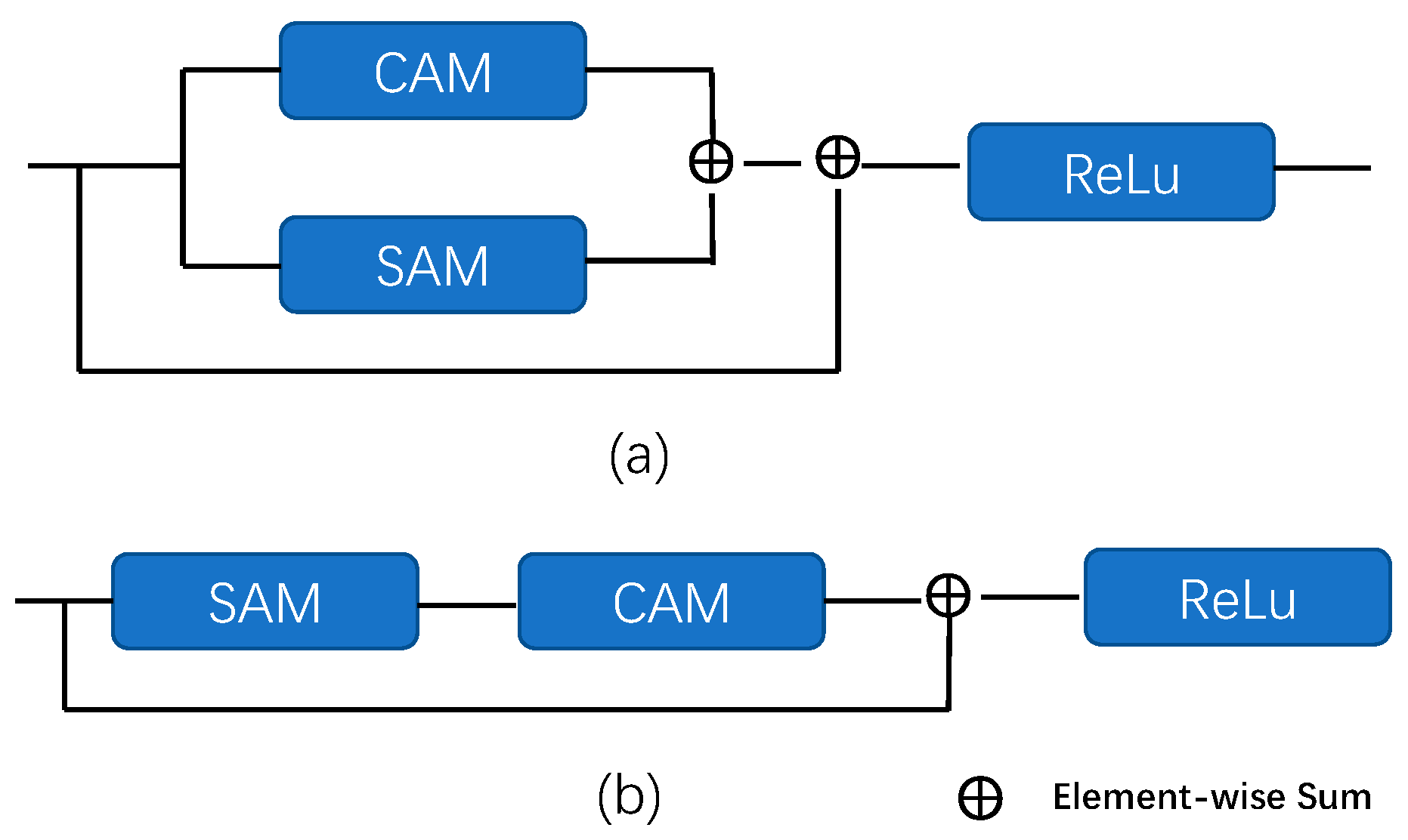
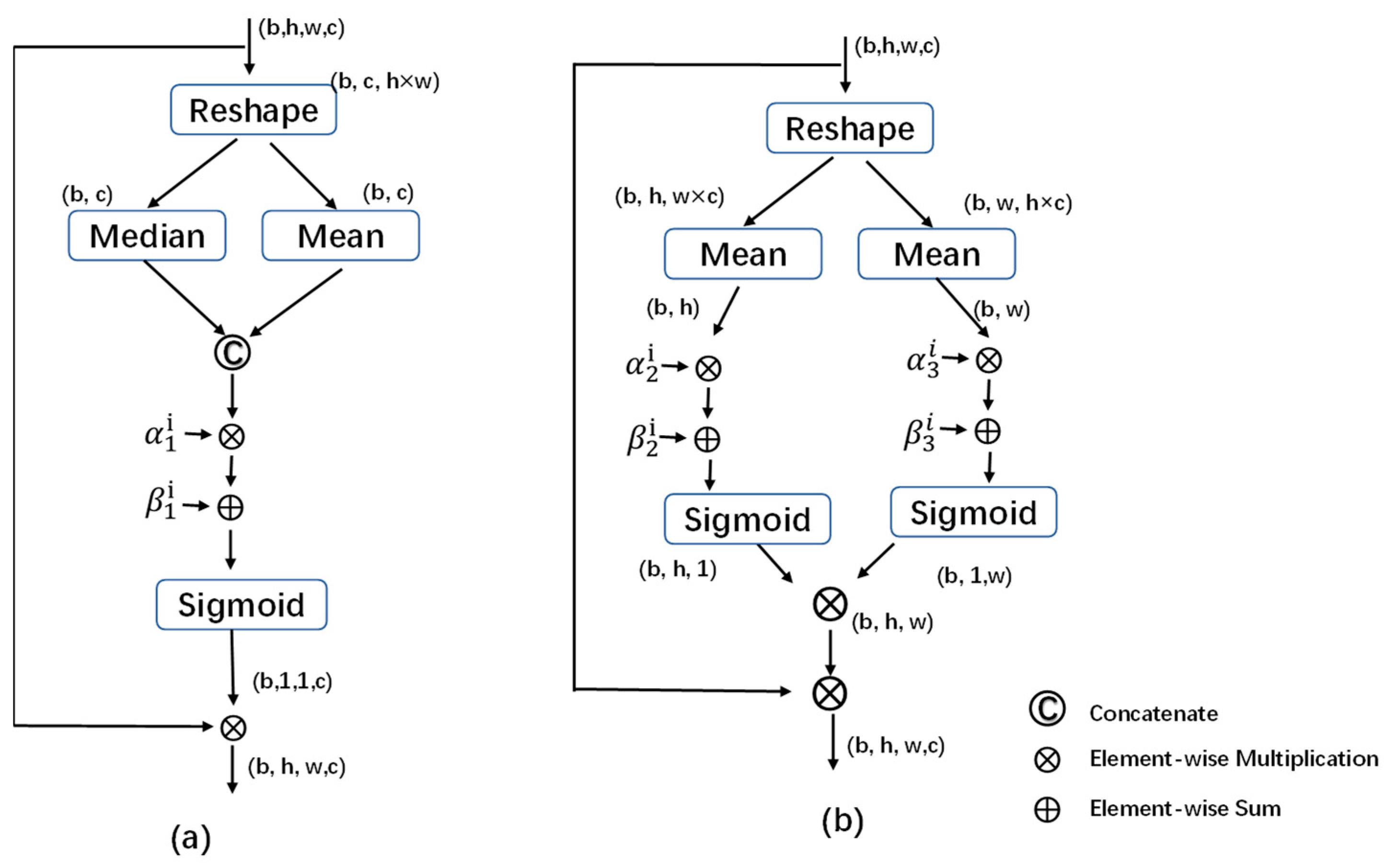
PCSAM connects two attention modules in parallel and normalizes them with the ReLU activation function, as shown in Figure 3a. In addition, we also considered the effect of serial connection in the ablation study, and Figure 3b shows the way to connect the two attentions in series. Figure 4 shows the detailed structure of the two attention modules of PCSAM, and Figure 4a is the channel attention module. We reshape the input feature map from X b × h × w × c to b × c × h w to reduce the dimension more conveniently and capture the weight information on the channel dimension. The median and mean values are calculated on the last dimension, respectively, which are used to reduce the dimension and obtain the global information of the feature map. The size of the feature map becomes b × c . After concatenating the two feature maps obtained in different ways, linear regression is performed on the feature maps using two groups of learnable parameters, α 1 i and β 1 i . At the same time, the number of channels is followed by a recovery to the number of input feature map channels. Finally, the nonlinearization result is obtained through the Sigmoid activation function and is multiplied element by element with the input feature map X to obtain a new feature map after channel attention screening. The overall process is expressed by the formula:
Y = X     σ ( α 1 i C o n c a t e ( M e d i a n ( X ) , M e a n ( X ) ) + β 1 i )
where Y denotes the output feature map, X denotes the input feature map, denotes element-wise multiplication, σ denotes the Sigmoid activation function, Concate represents concatenation in the last dimension of the feature map, Median denotes the median in the last dimension, Mean means the average in the last dimension, and α 1 i and β 1 i are the two learnable parameters. Note that the reshaping steps are omitted here.
Figure 4b shows the improved spatial attention. It is used to capture the pixels that need attention in the height and width dimensions of the feature map. In this spatial attention module, we construct two branches for the height and width dimensions, respectively. As can be seen from Figure 4a, the overall structure is similar to that of the channel attention module, but the dimensionality reduction is performed by averaging over both branches. The size of the feature maps of the left and right branches after dimensionality reduction are b × h and b × w , respectively. Then, the learnable parameters are α 2 i , β 2 i and   α 3 i , β 3 i , respectively. Finally, the weight information learned from the two branches is fused and reshaped into the size b × h × w of the input feature map, and then weighted in a point-by-point multiplication to obtain the feature map screened by the spatial attention mechanism. The overall process is expressed by the formulas:
Y 1 = σ ( α 2 i   M e a n ( X ) + β 2 i )
  Y 2 = σ ( α 3 i   M e a n ( X ) + β 3 i )
Y = X     ( Y 1     Y 2 )
where Y 1 and   Y 2 denote the output weights of the two branches, i.e., the result after applying attention to the height and width dimensions of the feature map, respectively; denotes element-wise multiplication; σ denotes the Sigmoid activation function; and α 2 i ,   α 3 i ,   β 2 i   a n d   β 3 i   are all learnable parameters. Note that the step of reshaping is omitted here.

3.3. MSFM

The structure of MSFM is depicted in Figure 5, where each convolution is followed immediately by an atrous convolution. The atrous rates used in this design are 2, 6, 8, and 10. Specifically, a skip connection is made between the input of each standard convolution and the output of the atrous convolution, allowing for a greater concentration on contextual details. It concatenates all feature maps created by atrous convolution in the final dimension simultaneously to obtain feature information at various scales. As a result, the entire multi-scale fusion process has been completed. The module helps to focus on the global information at a given level and to prevent the loss of too much location information owing to the downsampling operation by serially connecting the layers with varying dilation rates in order to limit the number of downsampling and obtain a larger receptive field. The MSFM is set in the middle of the decoder architecture. With the noise reduced or eliminated thanks to the work of the first two PCSAMs, the ability of the MSFM to pick out and record informative multi-scale features is improved.

4. Experiments and Results

4.1. Datasets

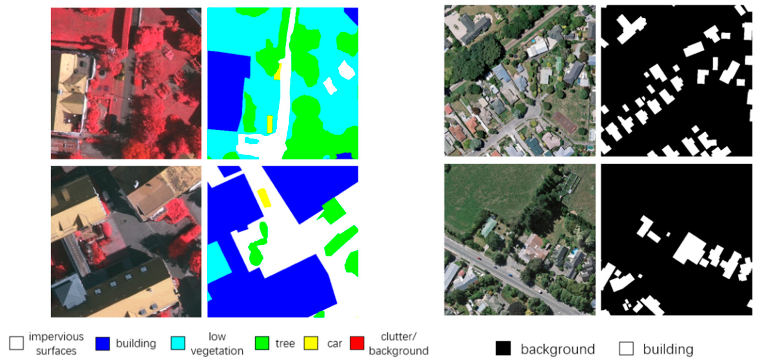
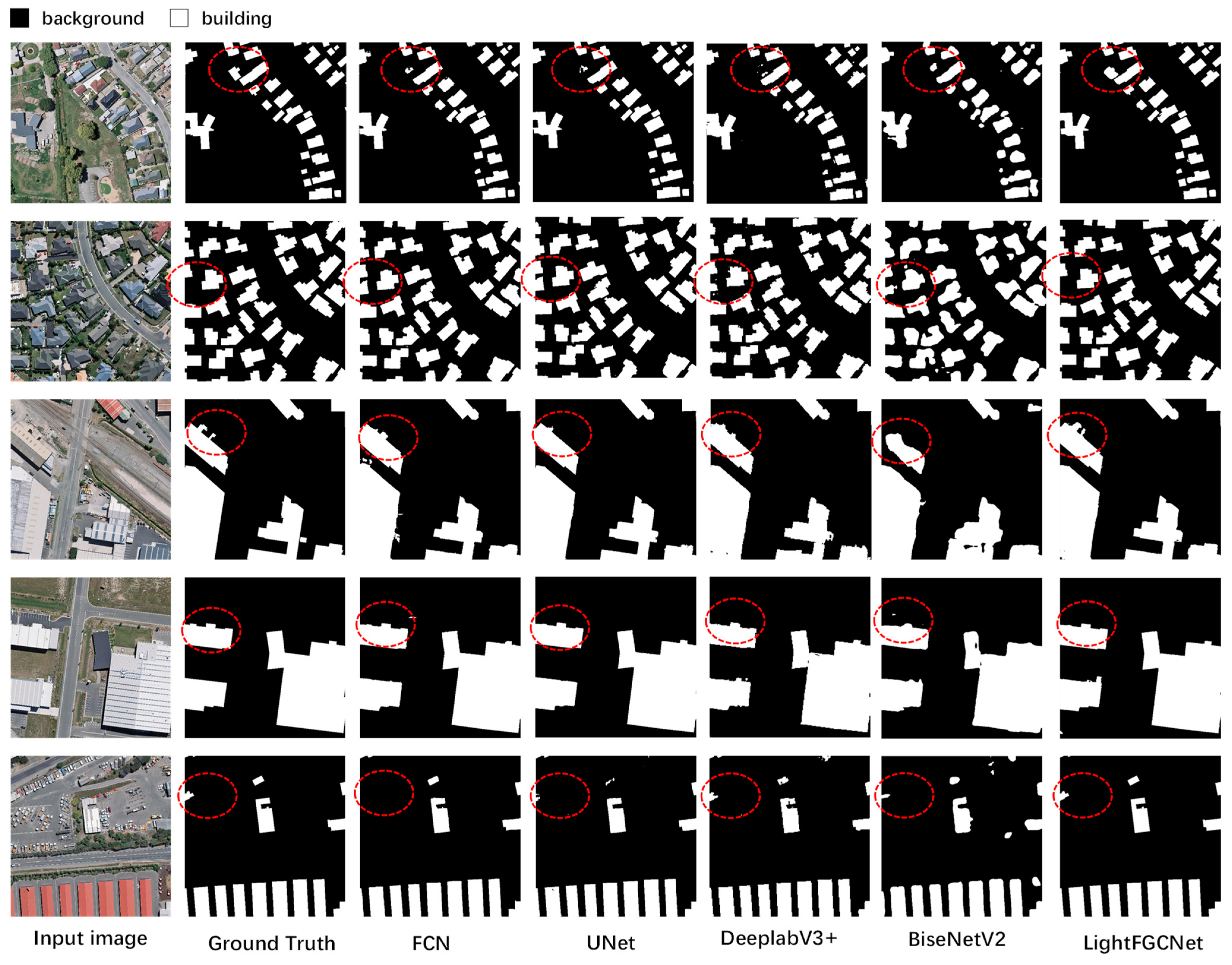
We chose the ISPRS Vaihingen [41] and WHU Building datasets [42], two open-source datasets for remote sensing image semantic segmentation, to measure the performance of our LightFGCNet. Examples of the dataset are shown in Figure 6. Impervious surface (white), buildings (blue), low vegetation (cyan), trees (green), cars (yellow), and background (red) make up the six types of terrain features in Vaihingen, a small village with many different types of buildings. The WHU Building dataset sponsored by Wuhan University is a selection of high-resolution photos clipped from aerial imagery obtained with the New Zealand Land Information Services and its labels include both background (black) and buildings (white).

4.1.1. ISPRS Vaihingen Dataset

There are a total of 33 images in the ISPRS Vaihingen dataset, with resolutions ranging from 1996 × 1996 to 3816 × 2550 pixels. With 9 cm of spatial resolution for both the top-level orthophoto image and the digital surface model (DSM) that is built from it using dense image matching algorithms, each image is retrieved from the bigger original. The DSM is in a single-band of TIFF format, while the remote sensing image format is 8-bit TIFF consisting of three bands, i.e., near-infrared, red, and green. The entire dataset is divided into a training set of 16 images and a test set of 17 images. To assist the training and evaluation of the model, we cropped each image into several small patches with a resolution of 384 × 384 pixels. There are 817 and 2219 patches in the training set and test set, respectively. It should be noted that, to minimize the effect of cropping, the adjacent patches in the training set are generated with 72 pixels overlap and 192 pixels for the patches of the test set.

4.1.2. WHU Building Dataset

The WHU Building dataset was published by the Photogrammetry and Computer Vision (GPCV) research team led by Shunping JI at Wuhan University. About 22,000 buildings with an original ground resolution of 0.075 m are included in the WHU Building dataset. Currently, the images are resampled to a ground resolution of 0.3 m and are cropped into 8188 images of 512 × 512 pixels, with 4736 images used as the training set, 1036 as the validation set, and 2416 images as the test set.

4.2. Experimental Setup and Evaluation Metrics

The Adam optimization function and the cross entropy loss function are chosen for all experiments. The learning rate is initialized to 0.001. If there is no improvement in the loss value on either the training or validation set after five epochs, the learning rate is decreased to 0.1 times the current value. The training is stopped if there is still no improvement after 50 epochs. Our experiments are based on Windows 10, Python 2.7, TensorFlow 2.9, and NVIDIA GeForce RTX 3060. The number of parameters and floating point operations (FLOPs) is used to measure the complexity of the networks, and the mean F1 score, overall accuracy (OA), and mean intersection over union (mIoU) are used to measure the effectiveness of the segmentation results. These metrics are calculated as follows:
F 1 = 2 × P r e c i s i o n × R e c a l l P r e c i s i o n + R e c a l l ;
P r e c i s i o n = T P T P + F P ;
R e c a l l = T P T P + F N ;
I o U = T P T P + F P + F N   ;
O A = T P + T N P + N
where P, N, TP, TN, FP, and FN represent the positive, negative, true positive, true negative, false positive, and false negative pixels in the prediction map, respectively. The precision is the proportion of TPs in the total positive prediction. The recall represents the percentage of TPs over the total positive pixels. The F1 score is the weighted average of recall and precision, which involves both FP and FN. The IoU is the intersection of the prediction and ground truth over their union of the image and the OA represents the ratio of the number of correctly predicted pixels to the total number of pixels.

4.3. Ablation Study

We conduct ablation tests on the Vaihingen dataset to show the viability of our method. LightFGCNet-C48 is used as the default architecture for all trials, where ‘C48’ indicates the number of output channels of the first stage, i.e., 48. All other hyperparameters are also set to be consistent. In this section, we will evaluate the effectiveness of our proposed LightFGCNet, including three aspects: the parallel channel spatial attention module (PCSAM), the multi-scale fusion module (MSFM), and the channel number of basic blocks.

4.3.1. Parallel Channel Spatial Attention Module

To reduce noise, LightFGCNet combines two attention modules into a PCSAM. We conduct experiments to further examine how the type of attention module used and the method to combine two attention modules affect the network performance: (1) channel attention only (LightFGCNet-channel), (2) spatial attention only (LightFGCNet-spatial), (3) serial connection of two attention modules (LightFGCNet-serial), and (4) parallel connection of two attention modules (LightFGCNet-parallel). Figure 3 demonstrates the different ways of connecting channel attention and spatial attention. When comparing the effect of one of the modules, it is sufficient to remove the corresponding module from it.
According to the experimental findings in Table 1, our suggested LightFGCNet performs better than other forms when using parallel channel and spatial attention. There is a 1.83% increase in mean F1 and a 1.58% improvement in OA compared to when only spatial attention is used. Compared to conventional channel attention, mean F1 and OA are also enhanced by 1.12% and 0.59%, respectively. The importance of channel attention in the LightFGCNet network is noticeably greater than that of spatial attention. One possible explanation is that the ability of spatial attention may be diminished as a result of the network downsampling more frequently and losing more spatial position information. Nevertheless, the results demonstrate that the performance of employing two attentions is substantially better than using only one, experimentally demonstrating the necessity of selecting both the channel and spatial dimensions of the feature map. Moreover, the parallel connection enhances mean F1 and OA by 0.5% and 0.4%, respectively, when compared to the serial connection. In comparison to the serial connection, in which the output of the second attention module is dependent on the output of the first, the parallel connection enables the two modules to independently complete the weight filtering of their respective dimensions and obtain the fully filtered feature maps by summing, albeit at the expense of a small reduction in computational efficiency.
To demonstrate that our proposed PCSAM can fully function in the decoder, we replace and compare our PCSAM with the classical SE [22] and CBAM [43] and the recent ECA [24] attention module, respectively. Table 2 shows the performance of different attentions in our network, where w/o denotes without any attention module. SE and ECA are channel attention modules, while CBAM can be regarded as a serially arranged channel spatial attention module. From the table, it can be seen that the mean F1 and OA are improved by 1–2% after adding attention compared to the no-attention module. Adding PCSAM improves mean F1 and OA by 1.33% and 0.78%, respectively, compared to CBAM, which proves from another aspect that parallel channel spatial attention is more effective compared to serial one. In addition, compared with adding only the channel attention module, the performance of further improvement is not significant after adding the channel spatial attention module. It is evident that channel attention plays a more important role in the network.

4.3.2. Multi-Scale Fusion Module

The MSFM suggested in LightFGCNet is intended to direct the attention of the network toward additional multi-scale features. Therefore, we designed a comparative experiment to evaluate its effectiveness. LightFGCNet-w/o is for LightFGCNet without the MSFM, whereas LightFGCNet stands for the complete network.
Table 3 shows the F1 scores of the network with and without MSFM for each category in the Vaihingen dataset. The results demonstrate that the addition of the MSFM improves the F1 in each category by approximately 1%, particularly in the small sample and small-scale car F1 by 1.94%. This is advantageous for remote sensing imagery datasets, where the distribution of category scales is usually unbalanced. By extracting the feature map layer by layer using atrous convolutions with varying dilated rates, the network is able to collect multi-scale feature information as well as advanced semantic information. This resulted in an improvement in F1 across all categories, particularly for small target objects.

4.3.3. Channel Number of Basic Block

To strike a good balance between the number of parameters and the experimental result, we selected a network with 48 output channels for the initial stage. We also take into account how different numbers of channels might affect the efficiency of the network. Therefore, we switched to 32 and 64 channels in another ablation test, denoted as LightFGCNet-C32 and LightFGCNet-C64, respectively.
Table 4 shows the experimental results of LightFGCNet with various numbers of channels. With 48 channels, the number of parameters and FLOPs is roughly half as high as with 32 channels and the mean F1 and OA are improved by 1.19% and 1.07%, respectively. The FLOPs of the network with 64 channels are 17.8G more than those of the network with 48 channels. However, the mean F1 and OA only improved by 0.99% and 0.91%, respectively. This illustrates the minor benefit given to the network simply by increasing the number of channels in the feature map. LightFGCNet-C64 requires more hardware resources for training and lengthening training time per epoch but achieves slim segmentation performance enhancement. LightFGCNet-C48 is used since it is less computationally intensive while still providing adequate segmentation accuracy.

4.3.4. Comparison of Encoders

In this paper, our proposed method uses an encoder consisting of a few simple convolutional blocks. To further reduce the number of parameters, we used depth-wise separable convolutions. Our encoder achieves an effective balance between feature extraction and the number of parameters. In addition, to adequately perceive the advantages of the proposed decoder compared to other decoder architectures, we replaced the encoder with ResNet50 [37] for comparison. Table 5 shows the quantitative results under different encoders. As can be seen from the table, when we replaced the encoder with ResNet50, the mean F1 and OA are very close to our proposed method, and even the mean F1 of LightFGCNet is improved by 0.26%, which proves that our proposed decoder is simple and efficient. Through comparison with the ResNet50 feature extraction, followed by direct bilinear interpolation upsampling, it can be seen that the performance of the network is greatly improved by adding the decoder.

4.4. Comparison with State-of-the-Art Models

We undertook comparative experiments on the Vaihingen dataset and WHU Building dataset, respectively, to evaluate the performance of LightFGCNet with other state-of-the-art networks. FCN, UNet, DeeplabV3+, BiseNetV2 [44], SMAF-Net [45], SCAttNet V2 [46], MF-Dfnet [47], SRANet [17], ASGASN [48] ESFNet [49], AttsegGAN [50], and CFENet [51] have been selected for the comparison.
Table 6 provides quantitative results from a variety of classical methodologies, and although SMAF-Net is the top performer for OA and mean F1, our proposed LightFGCNet-C48 improves mIoU by 5.17%. Compared to the classical lightweight approach BiseNetV2, which has the fewest parameters and FLOPs, our proposed method achieves improvements of 5.9% in OA, 8.66% in mean F1, 9.04% in recall and 10.83% in mIoU. In addition, LightFGCNet-C48 has a lower number of parameters and FLOPs compared to other classical approaches. The highest recall and mIoU demonstrate that our proposed strategy is superior in identifying the proper class of pixels. In general, it is able to obtain excellent performance with a lesser number of parameters and computational complexity. Table 7 displays the F1 Score for each category, mean F1, and mIoU within the Vaihingen dataset. Compared with other methods, LightFGCNet performs well on all classes of objects, which illustrates the suitability of the network for multi-objective semantic segmentation.
To evaluate the applicability of LightFGCNet in a variety of sectors, we also examined more conventional approaches on the WHU Building dataset. Table 8 displays the indicated values for recall, IoU, and F1 for buildings. The recall, F1, and IoU are increased by 7.13%, 7.55%, and 12.4%, respectively, when compared to the traditional lightweight network BiseNetV2. In comparison to ESFNet, another lightweight network used for building extraction, there is a rise of 4.53% in our IoU. The published ESFNet does not provide the other evaluation indicators. The F1 and IoU of our proposed approach perform better than UNet, another baseline network, by a margin of 0.65% and 0.82%, respectively. It is demonstrated on another dataset that our proposed method is able to provide state-of-the-art performance in terms of both the computational complexity and segmentation performance of the network.

5. Discussion

The parameters and FLOPs of the conventional networks on the Vaihingen dataset are provided in Table 7. Measurements provided by SMAF-Net and SCAttNet lack parameters and FLOPs. With the exception of BiseNetV2, we can see that our approach has the fewest parameters and FLOPs. The number of parameters and FLOPs are 0.14 M and 14.35 G higher than BiseNetV2, respectively. Moreover, LightFGCNet outperforms BiseNetV2 in terms of mIoU on the Vaihingen dataset, with a rise of 10.83%. Therefore, our proposed LightFGCNet can obtain higher segmentation accuracy with less computational complexity compared to other methods. To a certain extent, it has a modest number of parameters, which is significantly fewer than traditional semantic segmentation networks.
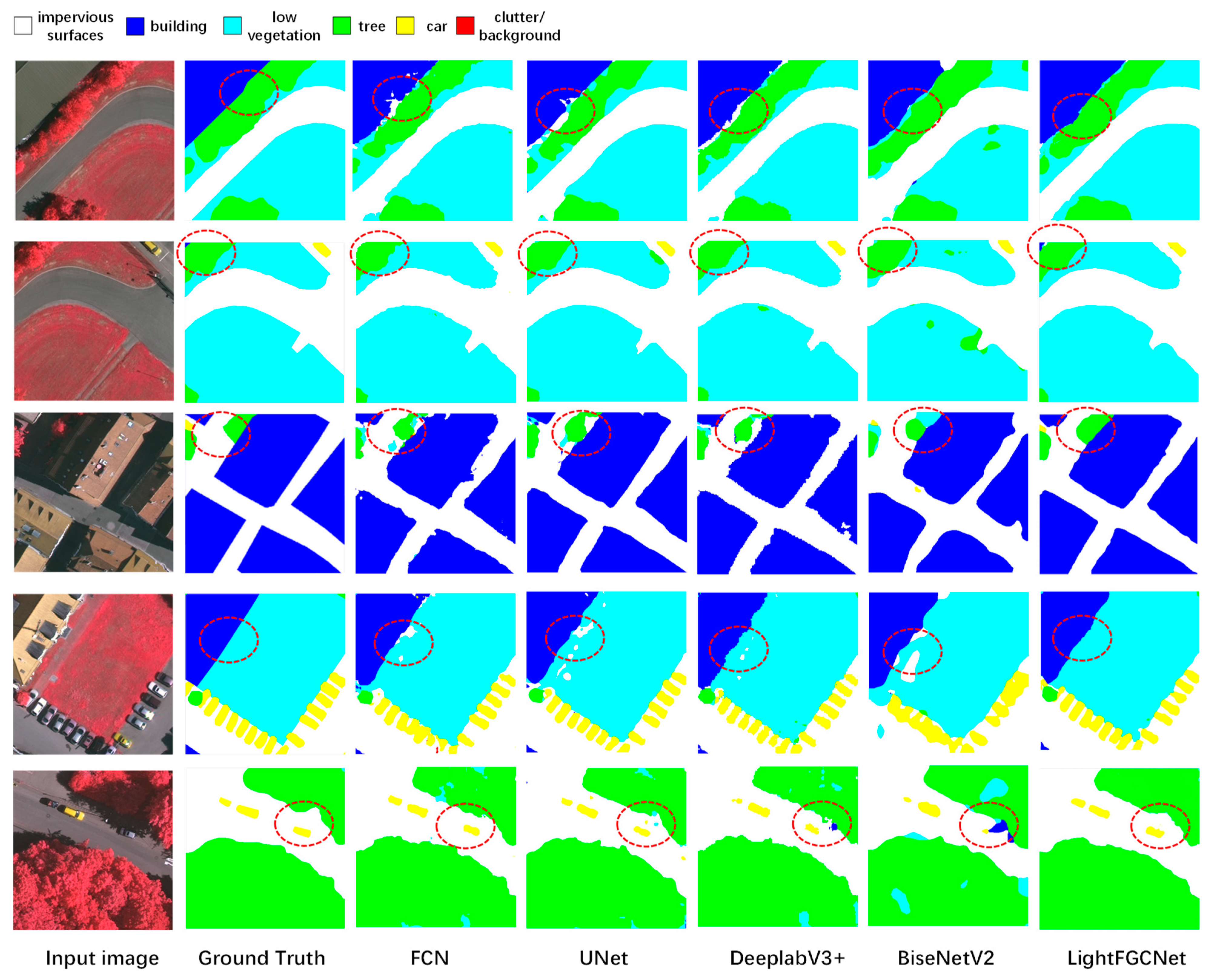
Figure 7 illustrates several ground truth images versus the outputs of FCN, UNet, DeeplabV3+, BiseNetV2, and the suggested network on Vaihingen. The red dashed lines mark the more obvious differences between the predicted images compared with the ground truth values. It is evident from the figure that our proposed strategy may greatly minimize the likelihood of misclassification in both multi-category and less-category scenarios, as shown by the prediction results of the five samples for different methodologies. Meanwhile, the segmentation’s border details are more finely sharpened. The experimental results show that the efficiency of remote sensing image semantic segmentation can be enhanced by paying attention to contextual details.
Figure 8 depicts the prediction results of a selection of approaches on the WHU Building dataset, with the bigger deviations denoted by red dashed lines. The first two samples demonstrate the capability of our approach to segment tiny targets. Light-FGCNet is able to accurately identify and segment small-scale targets when other conventional approaches mis-segment or segmentation is uncertain. The middle two samples demonstrate the segmentation performance on the finer features of large-scale objects. When compared to other lightweight networks, our approach allows for more distinct details around the apparatus’s edges. The final example demonstrates segmentation performance when dealing with numerous complex backgrounds. With a focus on the merging of contextual information and PCSAM noise filtering, LightFGCNet can distinguish small-scale targets from the background with accuracy and LightFGCNet is able to accurately detect small-scale targets from the background. Figure 8 demonstrates that our proposed method has a sharper edge contour than existing methods. This is due to the fact that LightFGCNet pays greater attention to the extraction of global contextual features and that merging high-resolution feature information might yield more boundary details. It can be seen that there is still potential for improvement in the segmentation of smaller pieces towards the perimeter of the building in comparison to the labels.

6. Conclusions

In the research, we proposed a novel CNN-based semantic segmentation network for remote sensing images. In contrast to the semantic segmentation of natural images, which is often accomplished using a single scale and a uniform distribution of characteristics across all objects, the targets in remote sensing images are typical of multiple scales and unevenly distributed. Therefore, contextual features play a significant role in the semantic segmentation of remote sensing images. Our lightweight network LightFGCNet focuses on global contextual information in place of CNN, which mostly deals with local information. LightFGCNet-C48, which uses 48 channels, not only achieves high segmentation performance but also has fewer parameters. The parallel-connected PCSAM can efficiently perform filtering in both channel and spatial dimensions. In addition, based on our experimental findings, the MSFM is effective in addressing issues of class imbalance and multiple scales. As a whole, our proposed method achieves very good performance on the ISPRS Vaihingen and the WHU Building datasets. Despite the fact that it achieves improved results on the performance of multi-scale targets segmentation and boundary details, there is still potential for enhancement in LightFGCNet’s computational cost. In our future work, we will further focus on this research direction.

Author Contributions

Y.C. proposed the main idea and reviewed and edited the manuscript; W.J. designed the methodology and wrote the manuscript; M.K. designed computer programs; M.W. synthesized the study data; T.W. and X.W. reviewed and edited the manuscript; M.T. supervised and took responsibility for the research activity planning and execution; L.X. scrubbed the data and maintained the research data; X.L. visualized the data; C.Z. verified the experimental design. All authors have read and agreed to the published version of the manuscript.

Funding

This work was funded by the National Natural Science Foundation of China (Grants No. 62176085 and 61673359), the Key Scientific Research Foundation of the Education Department of Province Anhui (Grant No. KJ2020A0658), the University Natural Sciences Research Project of Province (Grant No. KJ2021ZD0118), the Hefei University Talent Research Funding (Grant No. 20RC13), the Hefei University Scientific Research Development Funding (Grant No. 20ZR03ZDA), and the Hefei Specially Recruited Foreign Expert Support.

Data Availability Statement

The data and the code of this study are available from the corresponding author upon request.

Acknowledgments

The authors thank ISPRS for providing the Vaihingen dataset and GPCV, as well as WHU for providing the WHU Building dataset.

Conflicts of Interest

The authors declare that there are no conflict of interest regarding the publication of this paper.

References

  1. Zhang, T.; Su, J.; Liu, C.; Chen, W.-H. State and parameter estimation of the AquaCrop model for winter wheat using sensitivity informed particle filter. Comput. Electron. Agric. 2021, 180, 105909. [Google Scholar] [CrossRef]
  2. Long, J.; Shelhamer, E.; Darrell, T. Fully Convolutional Networks for Semantic Segmentation. In Proceedings of the IEEE Conference on Computer Vision and Pattern Recognition (CVPR), Boston, MA, USA, 7–12 June 2015; pp. 3431–3440. [Google Scholar]
  3. Ronneberger, O.; Fischer, P.; Brox, T. U-Net: Convolutional Networks for Biomedical Image Segmentation. In Proceedings of the 18th International Conference on Medical Image Computing and Computer-Assisted Intervention (MICCAI), Munich, Germany, 5–9 October 2015; pp. 234–241. [Google Scholar]
  4. Chen, L.C.; Papandreou, G.; Kokkinos, I.; Murphy, K.; Yuille, A.L. Semantic image segmentation with deep convolutional nets and fully connected crfs. arXiv 2014, arXiv:1412.7062. [Google Scholar]
  5. Chen, L.C.; Papandreou, G.; Kokkinos, I.; Murphy, K.; Yuille, A.L. DeepLab: Semantic Image Segmentation with Deep Convolutional Nets, Atrous Convolution, and Fully Connected CRFs. IEEE Trans. Pattern Anal. Mach. Intell. 2018, 40, 834–848. [Google Scholar] [CrossRef] [Green Version]
  6. Chen, L.C.; Papandreou, G.; Schroff, F.; Adam, H. Rethinking atrous convolution for semantic image segmentation. arXiv 2017, arXiv:1706.05587. [Google Scholar]
  7. Chen, L.C.; Zhu, Y.; Papandreou, G.; Schroff, F.; Adam, H. Encoder-Decoder with Atrous Separable Convolution for Semantic Image Segmentation. In Proceedings of the 15th European Conference on Computer Vision (ECCV), Munich, Germany, 8–14 September 2018; pp. 833–851. [Google Scholar]
  8. Dosovitskiy, A.; Beyer, L.; Kolesnikov, A.; Weissenborn, D.; Zhai, X.; Unterthiner, T.; Dehghani, M.; Minderer, M.; Heigold, G.; Gelly, S. An image is worth 16x16 words: Transformers for image recognition at scale. arXiv 2020, arXiv:2010.11929. [Google Scholar]
  9. Xu, Z.; Zhang, W.; Zhang, T.; Yang, Z.; Li, J. Efficient Transformer for Remote Sensing Image Segmentation. Remote Sens. 2021, 13, 3585. [Google Scholar] [CrossRef]
  10. Wu, T.; Tang, S.; Zhang, R.; Cao, J.; Zhang, Y. CGNet: A Light-Weight Context Guided Network for Semantic Segmentation. IEEE Trans. Image Process. 2021, 30, 1169–1179. [Google Scholar] [CrossRef]
  11. Xu, Z.; Zhang, W.; Zhang, T.; Li, J. HRCNet: High-Resolution Context Extraction Network for Semantic Segmentation of Remote Sensing Images. Remote Sens. 2021, 13, 71. [Google Scholar] [CrossRef]
  12. Sun, K.; Xiao, B.; Liu, D.; Wang, J. Deep High-Resolution Representation Learning for Human Pose Estimation. In Proceedings of the 32nd IEEE/CVF Conference on Computer Vision and Pattern Recognition (CVPR), Long Beach, CA, USA, 16–20 June 2019; pp. 5686–5696. [Google Scholar]
  13. Guo, M.H.; Xu, T.X.; Liu, J.J.; Liu, Z.N.; Jiang, P.T.; Mu, T.J.; Zhang, S.H.; Martin, R.R.; Cheng, M.M.; Hu, S.M. Attention mechanisms in computer vision: A survey. Comput. Vis. Media 2022, 8, 331–368. [Google Scholar] [CrossRef]
  14. Chen, W.; Zhu, X.; Sun, R.; He, J.; Li, R.; Shen, X.; Yu, B. Tensor Low-Rank Reconstruction for Semantic Segmentation. arXiv 2020, arXiv:2008.00490. [Google Scholar]
  15. Yang, M.; Yu, K.; Zhang, C.; Li, Z.; Yang, K. DenseASPP for Semantic Segmentation in Street Scenes. In Proceedings of the 31st IEEE/CVF Conference on Computer Vision and Pattern Recognition (CVPR), Salt Lake City, UT, USA, 18–23 June 2018; pp. 3684–3692. [Google Scholar]
  16. Huang, G.; Liu, Z.; van der Maaten, L.; Weinberger, K.Q. Densely Connected Convolutional Networks. In Proceedings of the 30th IEEE/CVF Conference on Computer Vision and Pattern Recognition (CVPR), Honolulu, HI, USA, 21–26 July 2017; pp. 2261–2269. [Google Scholar]
  17. Gao, L.; Qian, Y.; Liu, H.; Zhong, X.; Xiao, Z. SRANet: Semantic relation aware network for semantic segmentation of remote sensing images. J. Appl. Remote Sens. 2022, 16, 014515. [Google Scholar] [CrossRef]
  18. Zhao, H.; Zhang, Y.; Liu, S.; Shi, J.; Loy, C.C.; Lin, D.; Jia, J. PSANet: Point-wise Spatial Attention Network for Scene Parsing. In Proceedings of the 15th European Conference on Computer Vision (ECCV), Munich, Germany, 8–14 September 2018; pp. 270–286. [Google Scholar]
  19. Liu, S.; De Mello, S.; Gu, J.; Zhong, G.; Yang, M.H.; Kautz, J. Learning Affinity via Spatial Propagation Networks. In Proceedings of the 31st Annual Conference on Neural Information Processing Systems (NIPS), Long Beach, CA, USA, 4–9 December 2017; pp. 1521–1531. [Google Scholar]
  20. Zhang, L.; Xu, D.; Arnab, A.; Torr, P.H.S. Dynamic Graph Message Passing Networks. In Proceedings of the IEEE/CVF Conference on Computer Vision and Pattern Recognition (CVPR), Online, 14–19 June 2020. [Google Scholar]
  21. Sun, Q.; Liu, X.; Bourennane, S.; Liu, B. Multiscale denoising autoencoder for improvement of target detection. Int. J. Remote Sens. 2021, 42, 3002–3016. [Google Scholar] [CrossRef]
  22. Hu, J.; Shen, L.; Sun, G. Squeeze-and-Excitation Networks. In Proceedings of the 31st IEEE/CVF Conference on Computer Vision and Pattern Recognition (CVPR), Salt Lake City, UT, USA, 18–23 June 2018; pp. 7132–7141. [Google Scholar]
  23. Gao, Z.; Xie, J.; Wang, Q.; Li, P. Global second-order pooling convolutional networks. In Proceedings of the IEEE/CVF Conference on Computer Vision and Pattern Recognition(CVPR), Long Beach, CA, USA, 15–20 June 2019; pp. 3024–3033. [Google Scholar]
  24. Wang, Q.; Wu, B.; Zhu, P.; Li, P.; Zuo, W.; Hu, Q. ECA-Net: Efficient Channel Attention for Deep Convolutional Neural Networks. In Proceedings of the 2020 IEEE/CVF Conference on Computer Vision and Pattern Recognition (CVPR), Seattle, WA, USA, 13–19 June 2020; pp. 11531–11539. [Google Scholar]
  25. Qin, Z.; Zhang, P.; Wu, F.; Li, X. FcaNet: Frequency Channel Attention Networks. In Proceedings of the 18th IEEE/CVF International Conference on Computer Vision (ICCV), Online, 11–17 October 2021; pp. 763–772. [Google Scholar]
  26. Zhang, Y.; Li, K.; Li, K.; Wang, L.; Zhong, B.; Fu, Y. Image Super-resolution Using Very Deep Residual Channel Attention Networks. In Proceedings of the European Conference on Computer Vision (ECCV), Munich, Germany, 8–14 September 2018; pp. 286–301. [Google Scholar]
  27. Jaderberg, M.; Simonyan, K.; Zisserman, A.; Kavukcuoglu, K. Spatial Transformer Networks. In Proceedings of the 29th Annual Conference on Neural Information Processing Systems (NIPS), Montreal, QC, Canada, 7–12 December 2015; pp. 2017–2025. [Google Scholar]
  28. Hu, J.; Shen, L.; Albanie, S.; Sun, G.; Vedaldi, A. Gather-excite: Exploiting feature context in convolutional neural networks. In Proceedings of the Neural Information Processing Systems (NIPS), Montreal, QC, Canada, 3–8 December 2018; pp. 9423–9433. [Google Scholar]
  29. Zhu, Q.; Liao, C.; Hu, H.; Mei, X.M.; Li, H.F. MAP-Net: Multiple Attending Path Neural Network for Building Footprint Extraction From Remote Sensed Imagery. IEEE Trans Geosci Remote Sens. 2021, 59, 6169–6181. [Google Scholar] [CrossRef]
  30. Liao, C.; Hu, H.; Li, H.F.; Ge, X.M.; Chen, M.; Li, C.N.; Zhu, Q. Joint Learning of Contour and Structure for Boundary-Preserved Building Extraction. Remote Sens. 2021, 13, 1049. [Google Scholar] [CrossRef]
  31. Ma, N.; Zhang, X.; Zheng, H.-T.; Sun, J. ShuffleNet V2: Practical Guidelines for Efficient CNN Architecture Design. In Proceedings of the 15th European Conference on Computer Vision (ECCV), Munich, Germany, 8–14 September 2018; pp. 122–138. [Google Scholar]
  32. Howard, A.; Sandler, M.; Chu, G.; Chen, L.-C.; Chen, B.; Tan, M.; Wang, W.; Zhu, Y.; Pang, R.; Vasudevan, V.; et al. Searching for MobileNetV3. In Proceedings of the IEEE/CVF International Conference on Computer Vision (ICCV), Seoul, Republic of Korea, 27 October–2 November 2019; pp. 1314–1324. [Google Scholar]
  33. Zhou, D.; Hou, Q.; Chen, Y.; Feng, J.; Yan, S. Rethinking Bottleneck Structure for Efficient Mobile Network Design. In Proceedings of the European Conference on Computer Vision (ECCV), Edinburgh, UK, 23–28 August 2020; pp. 680–697. [Google Scholar]
  34. Zhang, Z.Q.; Lu, W.; Cao, J.S.; Xie, G.Q. MKANet: An Efficient Network with Sobel Boundary Loss for Land-Cover Classification of Satellite Remote Sensing Imagery. Remote Sens. 2022, 14, 4514. [Google Scholar] [CrossRef]
  35. Chen, L.L.; Zhang, H.M.; Song, Y.J. Extraction of Impervious Surface from High-Resolution Remote Sensing Images Based on a Lightweight Convolutional Neural Network. Wirel. Commun. Mob. Comput. 2022, 2022, 8636973. [Google Scholar] [CrossRef]
  36. Wang, L.B.; Li, R.; Zhang, C.; Fang, S.H.; Duan, C.X.; Meng, X.L.; Atkinson, P.M. UNetFormer: A UNet-like transformer for efficient semantic segmentation of remote sensing urban scene imagery. ISPRS J. Photogramm. Remote Sens. 2022, 190, 196–214. [Google Scholar] [CrossRef]
  37. He, K.; Zhang, X.; Ren, S.; Sun, J. Deep Residual Learning for Image Recognition. arXiv 2015, arXiv:1512.03385. [Google Scholar]
  38. Huang, H.G.; Chen, Y.P.; Wang, R.S. A Lightweight Network for Building Extraction From Remote Sensing Images. IEEE Trans. Geosci. Remote Sens. 2022, 60, 5614812. [Google Scholar] [CrossRef]
  39. Lv, L.; Guo, Y.Y.; Bao, T.F.; Fu, C.Q.; Huo, H.; Fang, T. MFALNet: A Multiscale Feature Aggregation Lightweight Network for Semantic Segmentation of High-Resolution Remote Sensing Images. IEEE Geosci. Remote Sens. Lett. 2021, 18, 2172–2176. [Google Scholar] [CrossRef]
  40. He, K.; Zhang, X.; Ren, S.; Sun, J. Spatial Pyramid Pooling in Deep Convolutional Networks for Visual Recognition. In Proceedings of the 13th European Conference on Computer Vision (ECCV), Zurich, Switzerland, 6–12 September 2014; pp. 346–361. [Google Scholar]
  41. ISPRS Vaihingen Dataset. Available online: https://www.isprs.org/education/benchmarks/UrbanSemLab/2d-sem-label-vaihingen.aspx (accessed on 21 November 2022).
  42. Ji, S.; Wei, S. Building extraction via convolutional neural networks from an open remote sensing building dataset. Acta Geod. Cartogr. Sin. 2019, 48, 448–459. [Google Scholar]
  43. Woo, S.H.; Park, J.; Lee, J.Y.; Kweon, I.S. CBAM: Convolutional Block Attention Module. In Proceedings of the 15th European Conference on Computer Vision (ECCV), Munich, Germany, 8–14 September 2018; pp. 3–19. [Google Scholar]
  44. Yu, C.; Gao, C.; Wang, J.; Yu, G.; Shen, C.; Sang, N. BiSeNet V2: Bilateral Network with Guided Aggregation for Real-time Semantic Segmentation. arXiv 2020, arXiv:2004.02147. [Google Scholar] [CrossRef]
  45. Chen, J.; Zhu, J.; Sun, G.; Li, J.; Deng, M.J.I.G.; Letters, R.S. SMAF-net: Sharing multiscale adversarial feature for high-resolution remote sensing imagery semantic segmentation. IEEE Geosci. Remote Sens. Lett. 2020, 18, 1921–1925. [Google Scholar] [CrossRef]
  46. Li, H.; Qiu, K.; Chen, L.; Mei, X.; Hong, L.; Tao, C. SCAttNet: Semantic Segmentation Network With Spatial and Channel Attention Mechanism for High-Resolution Remote Sensing Images. IEEE Geosci. Remote Sens. Lett. 2021, 18, 905–909. [Google Scholar] [CrossRef]
  47. Zhang, S.C.; Wang, C.Y.; Li, J.H.; Sui, Y. MF-Dfnet: A deep learning method for pixel-wise classification of very high-resolution remote sensing images. Int. J. Remote Sens. 2022, 43, 330–348. [Google Scholar] [CrossRef]
  48. Yu, M.; Zhang, W.; Chen, X.; Liu, Y.; Niu, J. An End-to-End Atrous Spatial Pyramid Pooling and Skip-Connections Generative Adversarial Segmentation Network for Building Extraction from High-Resolution Aerial Images. Appl. Sci. 2022, 12, 5151. [Google Scholar] [CrossRef]
  49. Lin, J.; Jing, W.; Song, H.; Chen, G. ESFNet: Efficient Network for Building Extraction From High-Resolution Aerial images. IEEE Access 2019, 7, 54285–54294. [Google Scholar] [CrossRef]
  50. Wang, J.S.; Cai, M.R.; Gu, Y.F.; Liu, Z.; Li, X.X.; Han, Y.X. Cropland encroachment detection via dual attention and multi-loss based building extraction in remote sensing images. Front. Plant Sci. 2022, 13, 993961. [Google Scholar] [CrossRef]
  51. Chen, J.Z.; Zhang, D.J.; Wu, Y.Q.; Chen, Y.L.; Yan, X.H. A Context Feature Enhancement Network for Building Extraction from High-Resolution Remote Sensing Imagery. Remote Sens. 2022, 14, 2276. [Google Scholar] [CrossRef]
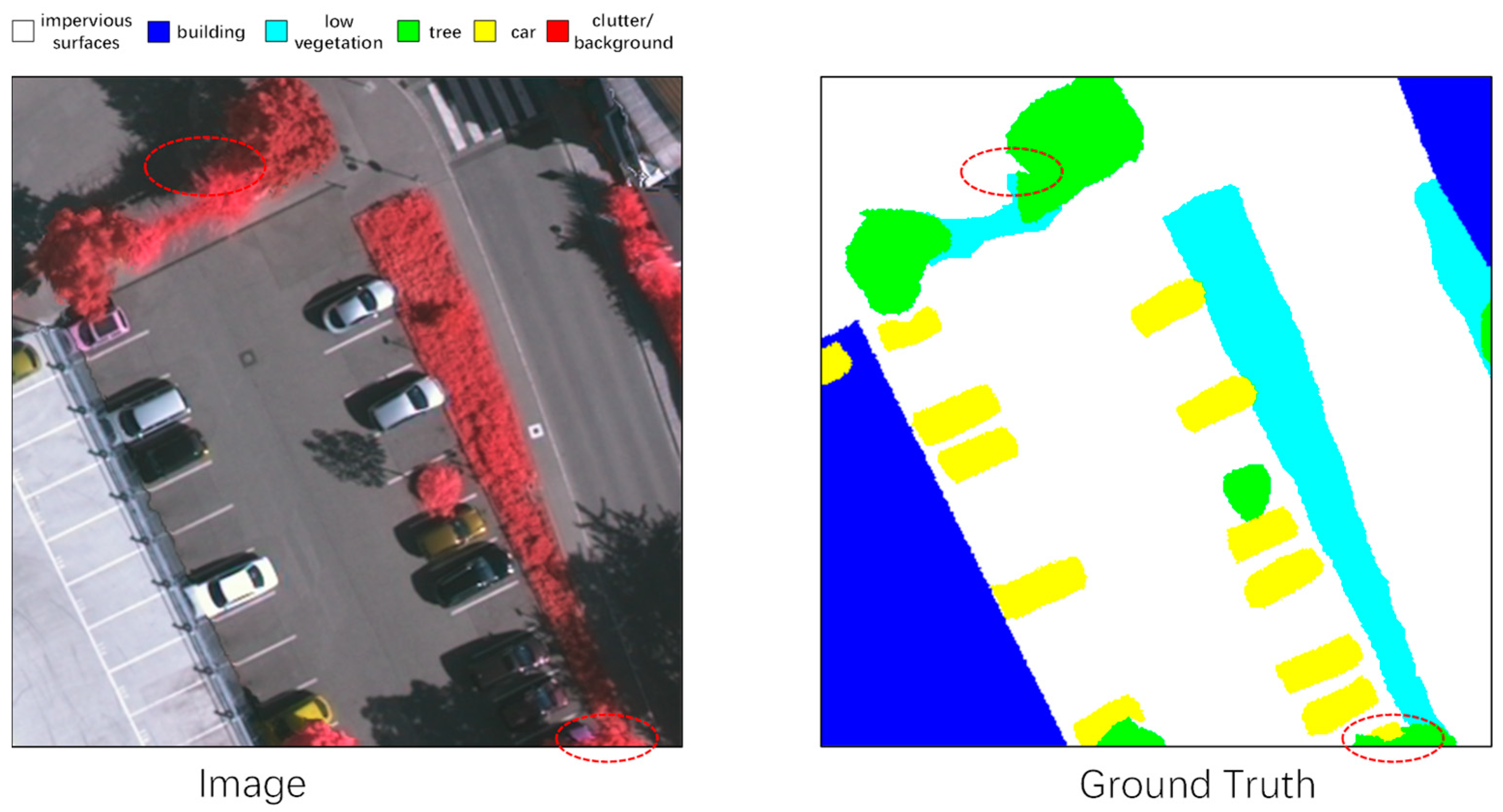
Figure 1. A high-resolution remote sensing sample image and the corresponding ground truth from the ISPRS Vaihingen dataset. The red circle shows the irregularity of the target boundary in the remote sensing images.
Remotesensing 14 06193 g001
Figure 2. The architecture of LightFGCNet.
Remotesensing 14 06193 g002
Figure 3. Overall structures of PCSAM with parallel and serial connections. (a) PCSAM connected in parallel; (b) PCSAM connected in serial.
Remotesensing 14 06193 g003
Figure 4. The detailed structure of PCSAM (a) for the channel attention module and (b) for the spatial attention module.
Remotesensing 14 06193 g004
Figure 5. The detailed structure of MSFM.
Remotesensing 14 06193 g005
Figure 6. Example images and labels of ISPRS Vaihingen (left) and WHU Building (right) datasets.
Remotesensing 14 06193 g006
Figure 7. Prediction images of different methods on ISPRS Vaihingen. The red dashed lines mark the more obvious differences.
Remotesensing 14 06193 g007
Figure 8. Prediction images of different methods on the WHU Building dataset. The red dashed lines mark the more obvious differences.
Remotesensing 14 06193 g008
Table 1. The ablation study of the attention module. The bold indicates the best data.
MethodMean F1 (%)OA (%)
LightFGCNet-channel81.0584.97
LightFGCNet-spatial80.3483.98
LightFGCNet-serial81.6785.16
LightFGCNet-parallel82.1785.56
Table 2. Ablation experiments on different attention comparisons, the w/o indicates no PCSAM. The bold indicates the best data.
MethodMean F1 (%)OA (%)
+w/o80.8684.49
+ECA81.4184.96
+SE81.6985.05
+CBAM80.8484.78
+PCSAM(ours)82.1785.56
Table 3. Ablation study of the multi-scale fusion module, the w/o indicates no MSFM. The bold indicates the best data.
MethodPre_Class F1-Score(%)Mean F1 (%)
Impervious
Surfaces
BuildingLow
Vegetation
TreeCar
LightFGCNet-w/o86.7590.1975.9383.5167.9580.87
LightFGCNet87.9191.4777.2684.3169.8982.17
Table 4. Ablation study of the channel number. The bold indicates the best data.
MethodMean F1 (%)OA (%)Parameters (M)FLOPs (G)
LightFGCNet-C3280.9884.491.4810.7
LightFGCNet-C4882.1785.563.1223.5
LightFGCNet-C6483.1686.474.7141.3
Table 5. Comparison of different encoders on our method with direct bilinear interpolation upsampling. The bold indicates the best data.
EncoderDecoderMean F1 (%)OA (%)
ResNet50standard76.3482.22
ResNet50ours81.9185.51
oursours82.1785.56
Table 6. Performance comparison on the Vaihingen dataset. The bold indicates the best data.
MethodRecall (%)mIoU (%)OA (%)Mean F1 (%)Parameters (M)FLOPs (G)
FCN83.0968.2484.6080.4712.7272.0
UNet83.0369.0384.7081.108.2367.8
DeeplabV3+83.3668.0184.7180.2114.3579.9
BiseNetV275.6259.6279.6673.512.989.15
SMAF-Net [45]-65.2888.4586.91--
SCAttNet V2 [46]-70.2085.4782.06--
MF-Dfnet [47]83.46-86.284.3614.34-
SRANet(50) [17]-66.3486.2777.95--
LightFGCNet-C4884.6670.4585.5682.173.1223.5
Table 7. mIoU, F1, and mean F1 on the Vaihingen dataset. The bold indicates the best data.
MethodmIoU(%)Pre_Class F1-Score(%)Mean F1 (%)
Impervious
Surfaces
BuildingLow
Vegetation
TreeCar
FCN68.2486.8390.5376.1283.8865.0280.47
UNet69.0387.4291.2575.1783.3368.3481.10
DeeplabV3+68.0187.0490.7676.0283.8963.3380.21
BiseNetV259.6281.9684.7370.4180.8949.5673.51
SMAF-Net [45]65.2891.8094.3081.2583.9583.2486.91
SCAttNet V2 [46]70.2089.1390.3480.0480.3170.5082.06
MF-DFNet [47]-88.893.178.484.077.584.36
SRANet(50) [17]66.3488.5292.0478.9685.7279.2177.95
LightFGCNet-C4870.4587.9191.4777.2684.3169.8982.17
Table 8. Recall, IoU, and F1 on the WHU Building dataset. The bold indicates the best data.
MethodRecall (%)F1 (%)IoU (%)
FCN93.5793.9188.51
UNet94.3394.2189.05
DeeplabV3+93.7793.3987.60
BiseNetV287.4487.3177.47
ASGASN [48]95.194.489.4
ESFNet [49]--85.34
AttsegGAN [50]-94.3589.07
CFENet [51]-92.6287.22
LightFGCNet-C4894.5794.8689.87
Publisher’s Note: MDPI stays neutral with regard to jurisdictional claims in published maps and institutional affiliations.