Article

An Object- and Shapelet-Based Method for Mapping Planted Forest Dynamics from Landsat Time Series

1
School of Information Engineering, China University of Geoscience, Beijing 100083, China
2
High Resolution Satellite Remote Sensing Application Department, Ningxia Institute of Remote Sensing Survey, Yinchuan 750021, China
3
Institute of Ecology, College of Urban and Environmental Sciences and Key Laboratory for Earth Surface Processes, Peking University, Beijing 100871, China
*
Author to whom correspondence should be addressed.
Remote Sens. 2022, 14(24), 6188; https://doi.org/10.3390/rs14246188
Submission received: 30 October 2022 / Revised: 26 November 2022 / Accepted: 4 December 2022 / Published: 7 December 2022
(This article belongs to the Section Forest Remote Sensing)

Abstract

:
Large-scale afforestation in arid and semi-arid areas with fragile ecosystems for the purpose of restoring degradation and mitigating climate change has raised issues of decreased groundwater recharge and ambiguous climatic benefits. An accurate planted forest mapping method is necessary to explore the impacts of afforestation expansion on fragile ecosystems. However, distinguishing planted forests from natural forests using remote sensing technology is not a trivial task due to their strong spectral similarities, even when assisted by phenological variables. In this study, we developed an object- and shapelet-based (OASB) method for mapping the planted forests of the Ningxia Hui Autonomous Region (NHAR), China in 2020 and for tracing the planting years between 1991 and 2020. The novel method consists of two components: (1) a simple non-iterative clustering to yield homogenous objects for building an improved time series; (2) a shapelet-based classification to distinguish the planted forests from the natural forests and to estimate the planting year, by detecting the temporal characteristics representing the planting activities. The created map accurately depicted the planted forests of the NHAR in 2020, with an overall accuracy of 87.3% (Kappa = 0.82). The area of the planted forest was counted as 0.56 million ha, accounting for 67% of the total forest area. Additionally, the planting year calendar (RMSE = 2.46 years) illustrated that the establishment of the planted forests matched the implemented ecological restoration initiatives over the past decades. Overall, the OASB has great potential for mapping the planted forests in the NHAR or other arid and semi-arid regions, and the map products derived from this method are conducive to evaluating forestry eco-engineering projects and facilitating the sustainable development of forest ecosystems.

Graphical Abstract

1. Introduction

Afforestation and reforestation have been the predominant means of countering forest degradation and mitigating climate change in recent decades [1], and the global forested area increased by 123 million ha between 1990–2020 [2]. Planted forests play valuable roles in reducing losses of natural forests, combating soil erosion and desertification, and boosting poverty alleviation strategies, especially in arid and semi-arid regions, which are among the most fragile ecosystems [3]. However, ecological restoration is a continuous successive process, and afforestation managers are eager to obtain the associated environmental benefits, resulting in negative effects such as increased water scarcity, declining soil quality, and low tree survival rates [4]. Assessments of forest cover often do not discriminate planted forests from natural forests, despite differences in structure and function (e.g., stand composition, biodiversity, and carbon sequestration), which underestimates the impacts of afforestation [5]. Therefore, baseline data depicting the accurate spatiotemporal distribution of planted forests are urgently needed to evaluate forestry eco-engineering programs and guide forestry management practices.
Numerous remote sensing studies have successfully identified planted forests. These studies can be divided into two categories of methods, the first of which is single-phase image classification. This method relies on abundant spectral signatures and texture variables in multi/hyper-spectral images to classify tree species at an individual or stand level, incorporating traditional classifiers (e.g., random forest [RF] and support vector machines [SVM]) or deep learning algorithms (e.g., convolutional neural networks [CNNs]) to optimize classification features [6,7]. Moreover, structural parameters, such as the canopy height, obtained from LiDAR data are partly complementary to the information from passive optical sensors for achieving higher classification accuracies [8,9]. Nevertheless, although high- and very-high-resolution images provide more spatial details, they increase the intra-class variability and data-processing costs for the discrimination of planted forests over large areas with high landscape heterogeneity. The second method is multi-temporal image classification based on distinctive periods in the growth process of planted forests. The intra-annual variations derived from phenological periods (i.e., leaf-on and leaf-off) increase the spectral separability [10]; thus, phenology-based algorithms are widely applied for discriminating tree plantations such as rubber, palm oil, and larch from other vegetation [11,12]. Alternatively, the distribution of plantations such as eucalyptus and tea were delineated according to the gap in the inter-annual time series caused by the selective logging or the artificial pruning phenological phase method [13,14], which revealed potential change events in planted forest mapping.
Here, planted forests are defined as trees or shrubs established by planting or seeding [15,16]. Accordingly, the main challenges of applying the above approaches to distinguish planted forests from natural forests over large geographical extents, especially in arid and semi-arid regions with high landscape heterogeneity, are the (1) spectral similarities between natural and planted forests and (2) intra-class variability of planted forests. The canopy spectral signals of mature planted forests are similar to those of natural forests, rendering them difficult to separate using single-phase imagery alone. In addition, differences in tree species, stand age, and disturbances (e.g., drought, fire) increase the intra-class variability of planted forests, thereby limiting the usefulness of intra-annual phenological characteristics in classification. In contrast, data over a long time span seem promising for avoiding these adverse impacts in the identification of planted forests [17]. Given that there is a low-vegetation-cover period triggered by site preparations (including soil clearing and amelioration) and planted forest seedlings with unenclosed canopies (intact natural forests maintain a relatively high vegetation cover), planted forests can be detected from natural forests [18]. Owing to the advantages of the longest historical archives (nearly 50 years) and the most comprehensive geographical record of Earth observations, Landsat data are appropriate for describing the inter-annual characteristics during the growth of forests. The normalized difference vegetation index (NDVI), which represents greenness, has been widely employed in forest cover monitoring [19]. Ye et al. [20] proposed a shapelet-based algorithm to discern rubber plantations from natural forests by detecting low-value segments (i.e., shapelets) of the Landsat-NDVI time series of forest pixels caused by planting activities. A shapelet is a sub-sequence that captures discriminative features while eliminating redundancy or even noise in a time series, providing deeper insights into the data [21]. Thus, the shapelet-based algorithm has been widely applied in image-outline classification, motion capture, and spectrographs [22].
Furthermore, planted forests are shaped relatively regular due to human intervention, and the forest structure is relatively simple [23]. Efforts to establish mixed species in recent decades are conducive to optimizing the forest structure and improving the stability and biodiversity of forestry ecosystems [24,25,26]. For medium- or high-resolution images (e.g., Landsat and Sentinel-2), the pixels capture only partial stand information, so they are not the optimal spatial units for describing the planted forests. More recently, object-based image analysis (OBIA) has made comprehensive use of contextual information and has mitigated the “salt-and-pepper effect,” thereby focusing attention on the object-based classification of either individual trees or forest stands [27]. Deng et al. [13] and Chen et al. [28] clustered pixels with the same features as homogenous plantation objects using image segmentation to reduce the effects of fragmentation and noise. The superiority of OBIA in image classification offers opportunities for the planted forest mapping and time-series monitoring of stand information over large areas.
In this study, according to the vegetation cover changes caused by the planting activities, we developed an object- and shapelet-based (OASB) method using the annual Landsat-NDVI time series and taking an example of the Ningxia Hui Autonomous Region (NHAR), to achieve two objectives: (1) develop and test the OASB method for distinguishing planted forests from natural forests in 2020 and (2) estimating the planting year from 1991 to 2020 to monitor the expansion of planted forests.

2. Materials and Methods

2.1. Study Area

The NHAR (104°17′–107°39′E, 35°14′–39°23′N) is located in the middle and upper reaches of the Yellow River in northwest China (Figure 1a). It encompasses five prefecture-level cities with a total area of 6.64 million ha. The terrain of the NHAR slopes gradually from southwest to northwest, with ravines and gullies (Figure 1b). The geographical structure is complex and diverse, surrounded by deserts on three sides and connected to the Loess Plateau in the south. It exists in the agro-pastoral transition zone, where natural forest resources are scarce and intensively distributed in Mount Helan, Mount Luo, and Mount Liupan, with Qinghai spruce (Picea crassifolia), Chinese pine (Pinus tabuliformis), and Prince Rupprecht’s larch (Larix principis-rupprechtii) as the dominant species [29,30]. Affected by the continental arid and semi-arid climate, the average annual precipitation (305 mm) is low and concentrated in the summer, yet the mean evapotranspiration (1800 mm) is high. Drought is an overriding limitation of plant growth in ecologically fragile regions [31]. Trees and shrubs, such as black locust (Robinia pseudoacacia L.), apricot (Prunus armeniaca L.), and aspen (Populus tremuloides Michx.), were established here to balance the ecological and economic benefits [32,33,34].

2.2. Methods

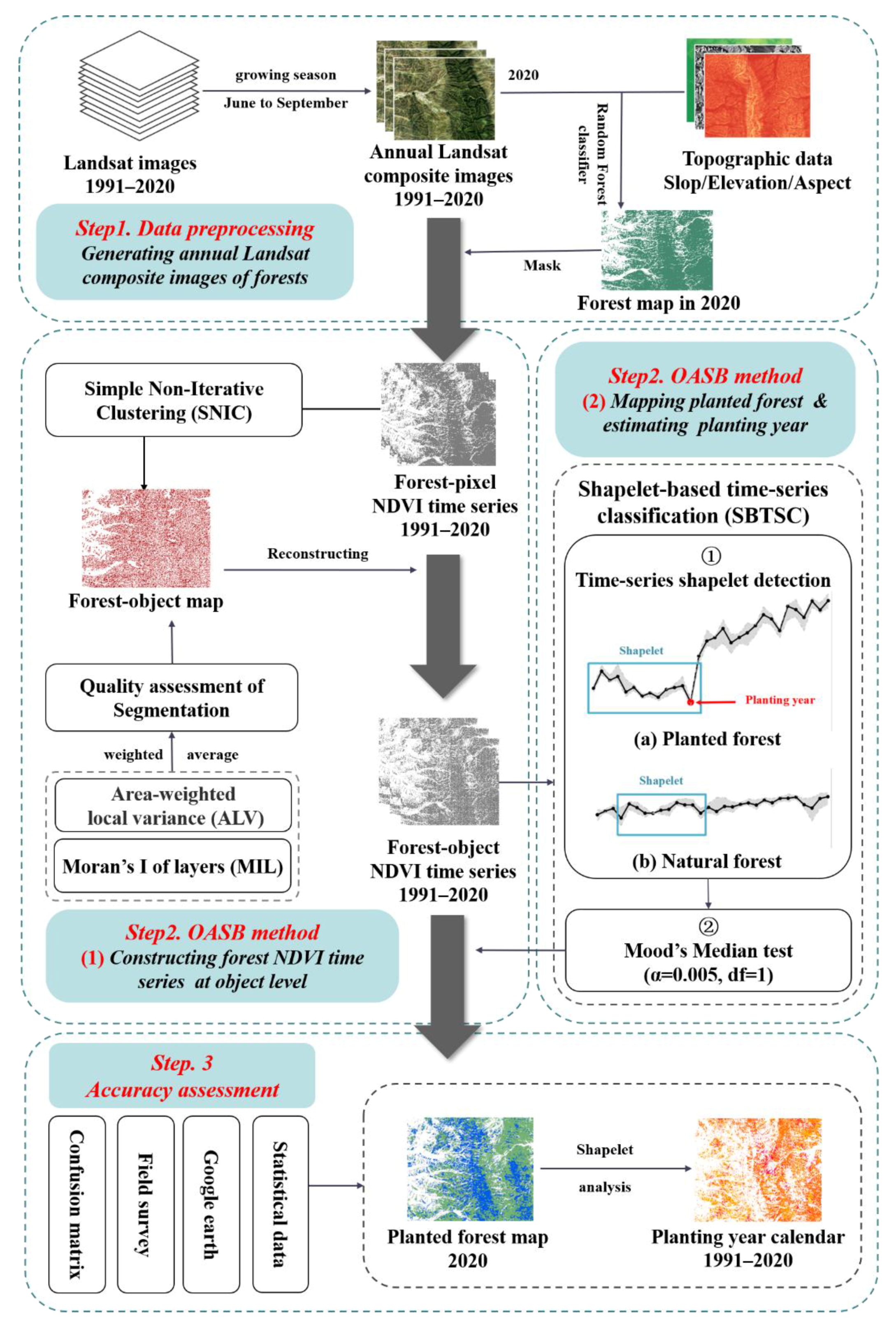
The general workflow consists of three main steps, as illustrated in Figure 2. The first step was preprocessing for building the annual Landsat-NDVI time series of the forested areas and the second step comprised the developed OASB method with two procedures: (1) simple non-iterative clustering (SNIC) to generate the forest objects and (2) shapelet-based time-series classification (SBTSC) to distinguish the planted forests from the natural forests and estimate the planting year. The forest maps were validated in the final step.

2.2.1. Data and Processing

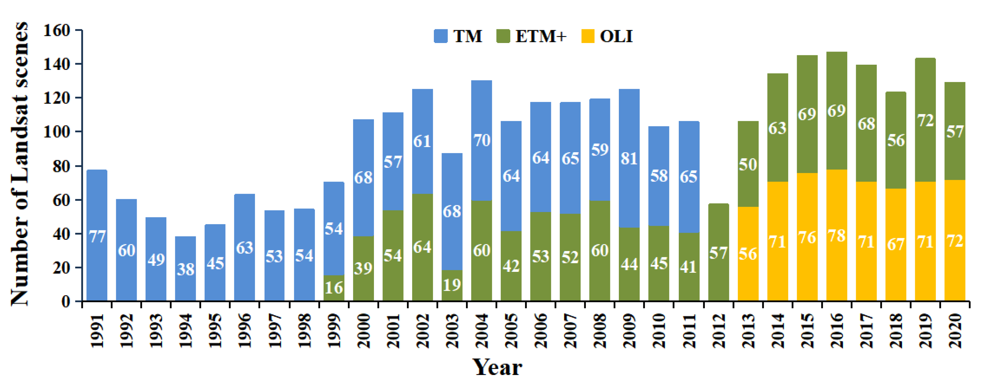
Free-access Landsat data were used as the primary data source in this study because of their long-term observations and relatively high spatial resolution [35,36]. The Google Earth Engine (GEE) is a cloud computational platform that enables users to access and process remote sensing data for planetary-scale geospatial analysis (https://earthengine.google.org/ (accessed on 16 April 2022)). To composite 30 cloud-free NHAR images for each year from 1991 to 2020, we collected Tier 1 surface reflectance satellite image products that had been atmospherically and topographically corrected from the Landsat-5 Thematic Mapper (TM; 1982–2013), Landsat-7 Enhanced Thematic Mapper (ETM+; 1999–present), and Landsat-8 Operational Land Imager (OLI; 2013–present) on the GEE platform. All images were selected during the forests’ growing season (from June to September) to reduce the impact of phenological factors [37]. An overview of all the Landsat data used in this study is shown in Figure 3. We then masked clouds, cloud shadows, and snow pixels from all the available images using CFMASK [38]. Finally, annual image composites were generated using a medoid approach, which is the value for a given band that is numerically closest to the median of all corresponding pixels among the images considered (all images within a provided annual data range) for a given image pixel. Time-series layer stacks of the NDVI images were subsequently processed from the collected annual Landsat composite images. The auxiliary data comprised the Shuttle Radar Topography Mission (SRTM) digital elevation model (DEM) from the GEE, and high-resolution images in Google Earth (Google Inc., Mountainview, CA, USA).
The forest map in 2020 served as a mask to remove non-forest pixels from the annual Landsat-NDVI time series. Here, we used the RF classifier to extract the forest (including natural and planted forests) distribution of the NHAR. Sample datasets are composed of 379 forest samples (including 247 planted forest samples) acquired via field study and 1259 points marked manually that rely on high-resolution images from Google Earth. In total, there are 613 forest samples. In addition to the spectral signatures (i.e., original spectral bands and spectral indices) of the Landsat composite images, textural features calculated using the gray-level co-occurrence matrix (GLCM) [39] and terrain characteristics are involved in the classification. To acquire features with higher sensitivity in the classification of land-cover types, the top 15 variables (Table 1) were selected according to their importance in the initial classification. Consequently, the overall accuracy (OA) of the final classification result was 89.1%. The forest area, including trees and shrubs, is 0.83 million ha, accounting for 16.0% of the total area of the study region; this is generally coincident with the statistical data that indicate the forest coverage of the NHAR in 2020 was 15.8%, as reported by the Ningxia Statistical Yearbook (http://tj.NHAR.gov.cn/ (accessed on 10 May 2022)).
Table 1. Top 15 variables ordered by their importance in the land-cover classification.
CategoryVariablesAcronymEquations or DescriptionsReferencesImportance
Topographic indexSlope-Slope/elevation calculated from digital elevation model (DEM) data -1
Elevation-4
Textural indexVariance (VAR)VAR_64 VAR = i = 1 j = 1 i μ 2 P i , j   [40]2
Sum average (SAVG)SAVG_64 7
SAVG_8 8
SAVG_3 9
SAVG_16 SAVG = k k = 2 2 G i , j = 1 G P i , j 12
SAVG_32 14
Correlation (CORR)CORR_64 CORR = i = 1 j = 1 ij P i , j μ x μ y σ x σ y 11
Spectral bandBlueB1--3
RedB3--6
Spectral indexModified normalized difference water indexMNDWI MNDWI = Green     SWIR 1 Green   +   SWIR 1 [41]5
Enhanced vegetation index EVI EVI = 2.5   ×   NIR     Red NIR   +   6   ×   Red     7.5   ×   Blue   +   1 [42]10
Normalized difference built-up indexNDBI NDBI = SWIR 1     NIR SWIR 1   +   NIR [43]13
Land surface water indexLSWI LSWI = NIR     SWIR 1 NIR   +   SWIR 1 [44]15
Variables in the textural index are calculated using GLCM based on corresponding window sizes; for instance, VAR _ 64 represents the textural index variance of a window of size 64. P i , j represents the probability of occurrences for the i , j   the entry in a joint probability distribution of pairs of gray levels, G represents the number of gray levels in the quantized image, and x and y represent the rows and columns of the GLCM, respectively.

2.2.2. Forest Object Generation

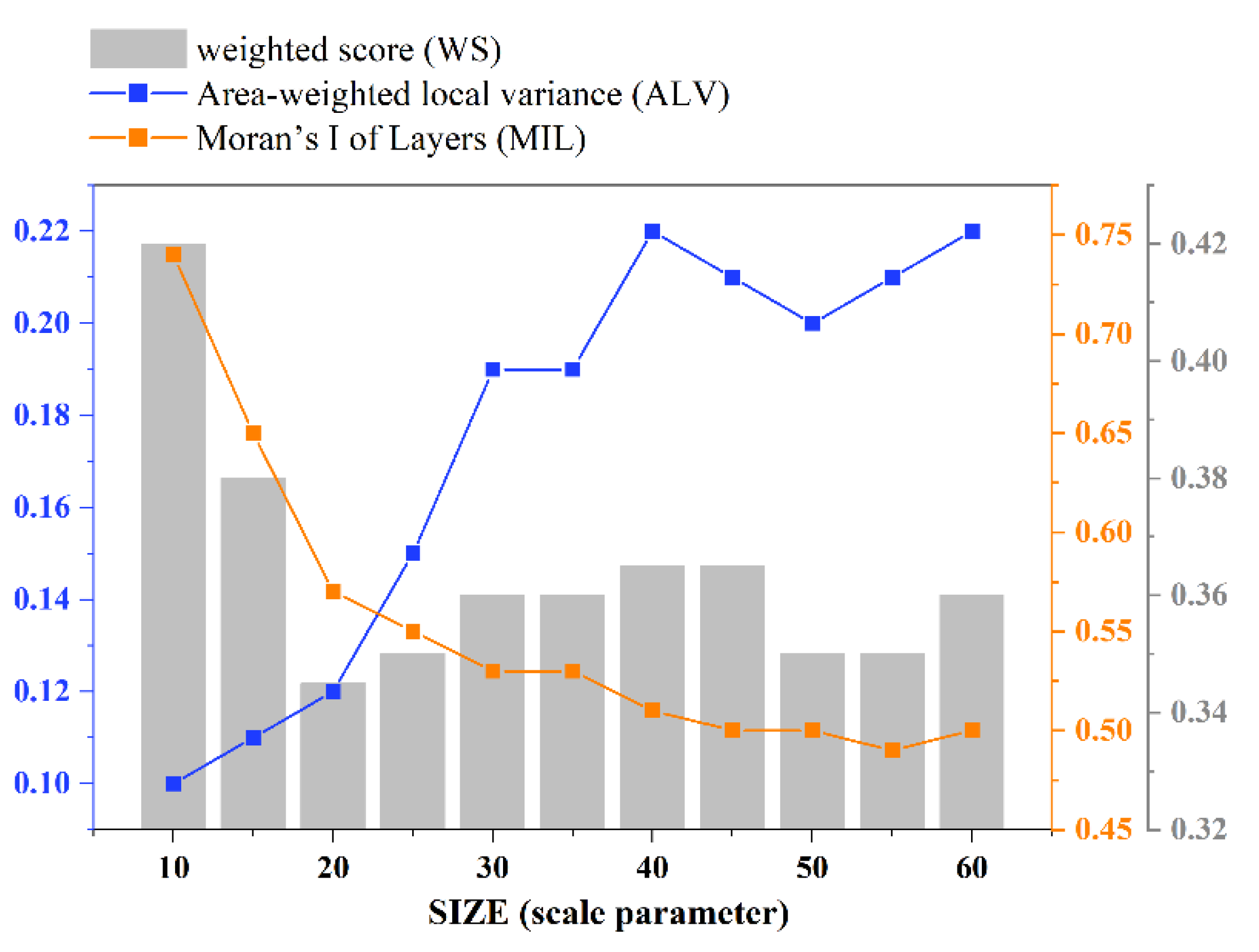
Image segmentation is a crucial and essential part of OBIA for creating objects from the connected pixels with similar features [45]. As for the segmentation algorithms, superpixel segmentation is an automatic technique that divides images into non-overlapping superpixels, performing well in remotely sensed images over a large scale because of few parameters and low memory requirements [46,47]. The SNIC method was adopted to yield homogenous superpixels by clustering contiguous pixels with similar NDVI trajectory patterns on the GEE. SNIC segmentation is an improved version of the widely used simple linear iterative clustering (SLIC) algorithm [48], which is non-iterative, requires less memory, and has a lower time complexity [49]. Segmentation quality has a significant effect on classification accuracy in OBIA, which is largely dependent on the parameter settings. Here, three parameters—size, compactness, and connectivity—are involved in the SNIC. As a scale parameter, size represents the average size of the forest objects, which is the most critical parameter for the algorithms. To ensure the homogeneity of the objects, 11 candidate sizes were, therefore, chosen for the sensitivity analysis. The compactness, with the capacity to constrain the object shape, was set to a relatively low value of 5, considering the irregular distribution and high landscape heterogeneity of the forested lands in the study area. We discovered that connectivity (4 or 8) had little effect on the segmentation results through testing; therefore, we set it to the slightly better performance value of eight neighbors.
Effective superpixels should have characteristics of a minimum intra-segment variance and maximum inter-segment difference. The two metrics, the area-weighted local variance (ALV; Formula (1)) and Global Moran’s I [50] of the layers (MIL; Formula (2)) were utilized to evaluate the intra- and inter-segment homogeneity, respectively [51]. Finally, the weighted score (WS; Formula. (3)) of the ALV and MIL was employed as a comprehensive indicator to clarify the performance of the SNIC algorithm under different scale values:
ALV = j = 1 l i = 1 n var ij     a ij / i = 1 n a ij l
where var ij and a ij represent the NDVI variance of superpixel i in layer j ; and l and n are the number of NDVI layers, and the total number of superpixels, respectively.
MIL = k = 1 l n i = 1 n j = 1 n w ij v i v ¯     v j v ¯ ( i = 1 n j = 1 n w ij )   i = 1 n v i v ¯ / l
where w ij represents a value (1 is adjacent and 0 is non-adjacent) of the adjacency matrix value between superpixels i and j ; and v i and v ¯ are the means of superpixels i and layer k , respectively.
WS = 0.5     ALV + 0.5     MIL
The minimum of WS corresponded to an optimum scale parameter of 20, as shown in Figure 4. As such, the SNIC was conducted under the optimal parameters to yield homogenous forest objects in the NHAR, and the superpixels spanning less than 0.5 hectares were subsequently eliminated according to the requirements outlined by [52]. Finally, the object-level NDVI (the pixel-level mean value) time series were built according to the SNIC superpixels.

2.2.3. Time-Series Shapelet Detection

Time-series shapelet detection includes an exhaustive search to generate a set of candidates and quality measurements to detect the best shapelet [20,53]. For a given annual NDVI time series T = t 1 ,   t 2 , , t 30 of the forest object, its candidate shapelet can be defined by the starting point p and length l , S p , l = t p , t p + 1 ,   ,   t p + l 1 min l max , whereas the corresponding remainder of the time series is defined as the non-shapelet N p , l = , t p 1 ,   ,   t p + l , min l max . We learned from local forestry experts that, in order to improve the survival rate of planted forests, trees were predominantly established through planting instead of seeding, and it took at least 4 years for the canopy cover to reach a relatively high level. Thus, the min of the shapelet was set to 4 ( max = 26 ) (1) to guarantee that the overwhelming majority of the planting initiatives could be examined and (2) to avoid misinterpreting changes induced by non-planting disturbances (e.g., clouds and cloud shadows) as planting activities.
Ye and Keogh [21] explained that the best shapelet divided a dataset into two groups as purely as possible. Time-series data were separated into two segments, shapelet and non-shapelet, so that the best shapelet in this study should have had the ability to minimize the intra-segment differences while maximizing the inter-segment differences, which helps to highlight the discrepancy between the pre- and post-planting stages. An indicator termed GAP (Formula (4)) was applied to evaluate the quality of candidates meeting the length criteria [54], and the best shapelet was defined as the candidate S p , l with the maximum value of GAP :
GAP p , l = m N p , l std N p , l m S p , l std S p , l
where m N p , l and m S p , l represent the mean of the non-shapelet and shapelet, respectively; std N p , l and std S p , l represent their standard deviations.

2.2.4. Mood Median Test

After implementing the detection algorithm, the best time-series shapelets were extracted for each forest object. Subsequently, a time-series object was identified as a planted forest if there was a significant difference between the shapelet and non-shapelet, or else it was classified as a natural forest. Here, the Mood median test (m-test) [55] was adopted to evaluate whether there was a significant difference in the NDVI medians for the two segments, which offered the benefit of being insensitive to outliers over the widely used Student’s test [56]. More specifically, a contingency table was employed to record the numbers in each group (shapelet or non-shapelet) below and above the median value of the NDVI time series [57], and the m-test statistic chi-square ( χ 2 ) derived from the contingency table acted as a measurement for the discrepancy between the normal status and variations. For a given time-series shapelet S p , l of a forest object, its statistic χ 2 was calculated using the following formula:
χ 2 = k = 1 r A k     n k / 2 2 n k / 2 + B k     n k / 2 2 n k / 2
where r represents the number of groups, which is 2 in this study. A k and B k are the number of NDVI values in group k that are above or below the median of the entire time series, respectively; n k is the stand sample size in each group. The greater the value of the statistic χ 2 , the more significant the difference.
Referring to the historical high-resolution images from Google Earth and the NHAR forestry expert advice, five typical cases were used to illustrate how the m-test differentiated the planted forests from the natural forests. The shapelet segments are highlighted by the blue rectangles. Figure 5a shows that the difference between the shapelets and non-shapelets is not significant ( χ 2 = 2.59 ) because there are fewer outliers during the NDVI trajectory of the intact natural forest. For the time series of the natural forests affected by cloud noise (Figure 5b), its shapelet consists of a noise point and the points with higher NDVI values on both sides of the noise. Owing to the insensitivity of the m-test to the abrupt change-point in the time series, its statistical value ( χ 2 = 2.84 ) was relatively low. Impeded by harsh environmental conditions, only those subjected to relatively mild disturbances can recover in the short term (within one to four years), whereas others damaged by severe destruction have little chance to survive. Thus, we depict a quickly recovered natural forest object from disturbances (e.g., logging, and irregular rainfall) in Figure 5c, whose discrepancy ( χ 2 = 4.91 ) between the two segments is marginally larger. A planted forest object converted from grassland or cropland with a high statistical value ( χ 2 = 11.07 ) is shown in Figure 5d. Its shapelet, composed of low NDVI values caused by the site preparation, the adaptation period after seedling transplantation, and a low canopy density stage, is considerably different from the non-shapelet representing high vegetation cover. Figure 5e illustrates an example of the significant differences ( χ 2 = 14.72 ) between the shapelet and non-shapelet of the planted forests converted from bare land, corresponding to the low-vegetation-cover period before forest maturity and the latter period of high vegetation cover. Essentially, the difference between the two segments induced by planting events is larger than that induced by image noises and most of the disturbances, so that the statistic χ 2 of the planted forests is larger than that of the natural forests.
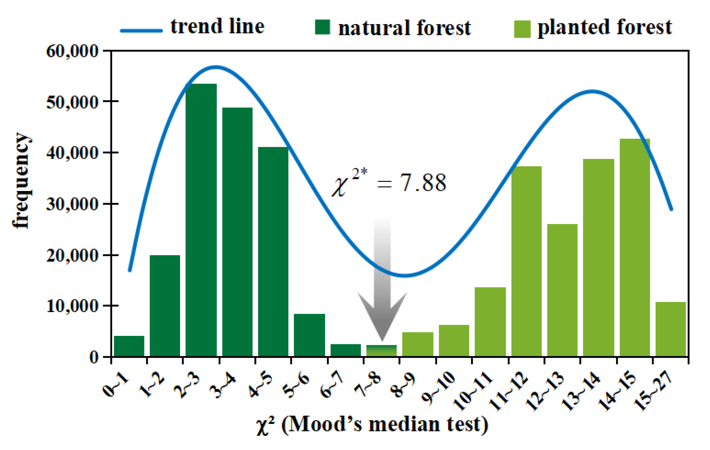
A time-series object was labeled as a planted forest if its statistic χ 2 exceeded a threshold determined using the significance level α and degree of freedom ( df ), illustrating that the NDVI median of the shapelet was distinctly lower than that of the non-shapelet. To determine the classification, the statistics χ 2 of all the forest objects were plotted in a frequency histogram, as shown in Figure 6. A demarcation is generated automatically in the interval of the lowest frequency ( χ 2 7 , 8 ). In accordance with the five typical cases, we set χ α = 0.005 , df = 1 2 = 7.88 as the final threshold. Therefore, a time-series object whose χ 2 exceeds 7.88 is defined as a planted forest; otherwise, it is defined as a natural forest.

2.2.5. Planting Year Estimation

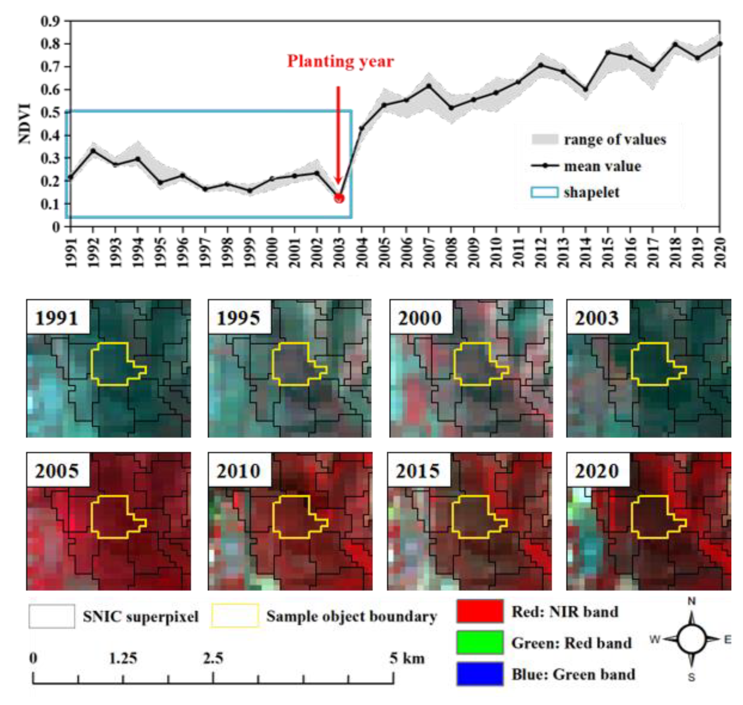
The establishing year of the planted forest can be estimated based on the interpretability of the time-series shapelets. As shown in Figure 7, the NDVI time-series data of the sample were segmented into shapelets and non-shapelets, corresponding to a low-vegetation-cover time comprising the site preparation and a high-vegetation-cover period for the growth of trees, respectively. In view of the definition of the planting year of rubber plantations in [20], in our study, the year of the planted forest establishment was defined as the last vertex on the time-series shapelet of a planted forest object. A vertex ( t v ) was decribed as a node of shapelet satisfiying the condition of t v = t v < t v 1   and   t v < t v + 1 , which is lower than the neighboring nodes. Since the trees started to grow after the transplanting of seedlings (or sowing), we chose the last vertex among the multiple ones that met the condition to characterize the time of planting. In addition, the Landsat imagery cutouts provide a visual interpretation of the changes in the land cover at the object level during the study period to illustrate the establishment of the planting year.

3. Results

3.1. Superpixel Segmentation of Forested Areas

A superpixel map of the NHAR forest areas in 2020 was generated using the SNIC algorithm, which was reduced by 2589 hectares compared to the original forest map after the de-fragment operation. One location (Figure 8a) was selected as an example to demonstrate the segmentation results (white polygons). Because the input data for the SNIC algorithm were the NDVI time series over three decades, the Landsat composite images for four years (1991, 2000, 2010, and 2020) served as backgrounds to illustrate the segmentation performance. Spatial segmentation captures the boundaries of the objects well in each image, which coincides with the visual inspection of the high-resolution images (Figure 8b) on Google Earth. In terms of the evaluation indicator, the ALV under the optimal scale (Figure 4) is less than 0.15, indicating that the homogeneity of the objects is reliable. Although some of the larger homogenous patches were divided into smaller parts, in general, the superpixels clustered by the neighboring pixels with the same NDVI trajectory patterns were consistent with the ground entities.

3.2. Planted and Natural Forest Mapping

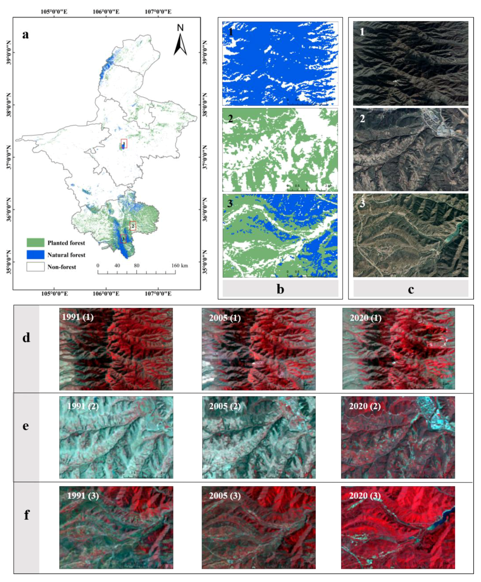
The resultant NHAR map in 2020 generated using the OASB method is displayed in Figure 9a, including three land-cover types: non-forest, planted forest, and natural forest. The distribution of the forests in the map is consistent with the fact that the natural forests are mainly located in the three mountains (see Section 2.1 above), whereas the planted forests are dispersed more widely. The planted forest area was 0.56 million ha, accounting for 67% of the total forest area. Simultaneously, three representative map locations were selected for enlargement to display more details based on the benefits offered by the forests. A natural barrier against sand invasion in the central arid area, formed by the forests on Mount Luo, is shown in Figure 9(b1). Figure 9(b2) displays an exemplary region for the Grain for Green Program (GGP), where ecological rehabilitation has achieved remarkable results over the past 20 years [58]. Moreover, in the region of Mount Liupan (Figure 9(b3)), the planted forests play a role in soil and water conservation. In addition to mountain areas, trees and plantations (mainly economic forests mixed with crops) have been established in plains areas.
A qualitative validation of the classification was undertaken via visual interpretation, which revealed that the forest map broadly matched the high-resolution images (Figure 9c); the multi-temporal Landsat images in 1991, 2005, and 2020 (Figure 9d–f) demonstrated that the color of the natural forest pixels remained red (or dark red) during the study period, while that of the planted forest pixels changed due to variations in the vegetation cover caused by the planting activities. Moreover, 100 sample points for each land-cover type by field survey and visual interpretation based on historical high-resolution images were screened to label the forest objects and non-forest regions as the reference data for the map validation. The confusion matrix (Table 2) derived from the 300 samples was used for accuracy assessment. The OA of the forest map was 87.3%, with a kappa coefficient of 0.82. For the planted forests, the overestimation error (19.0%) described by PA (81.0%) was greater than the underestimation error (8.0%) described by UA (92.0%), indicating that the proposed framework was slightly over-classified. The overestimation (17 out of 19) of the planted forest was mainly attributed to the high underestimation error (22.0%) of the non-forest area induced by the forest mask generation process.

3.3. Planting Year Characterization

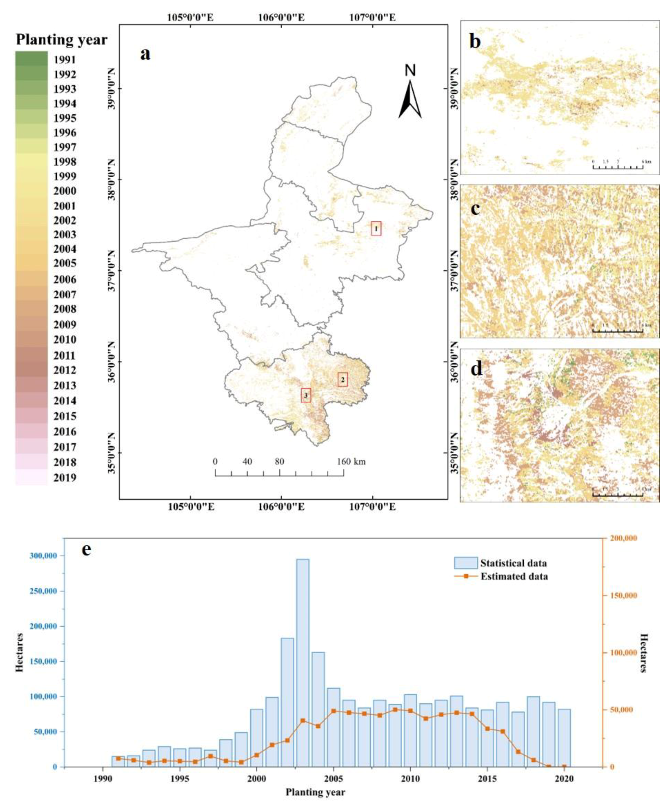
The expansion of the planted forests in the NHAR over the past three decades (1991–2020) is depicted in the planting year map (Figure 10a). All the forests planted before 1992 were marked as 1991. Three sites were purposely selected to display the map in detail. The planted forests in Figure 10b were mainly established during the period 2000–2010 (especially in 2005), and they have become an ecological protective screen to effectively block the invasion of the Mu Us desert. As shown in Figure 10c, economic forests, such as apricot (Armeniaca sibirica L.), were cultivated in the irrigated areas to increase rural incomes and improve the environment [59]. The years that these planted forests were established were not uniform, but they were mainly planted after 1998. Figure 10d shows that the site, as a water conservation area (rainfed agricultural system), has carried out continuous planting initiatives since the 1990s, with remarkable achievements around 2005 and 2012. The annual planting area (1991–2020) (in Figure 10e) derived from the planting year map reveals that 93.1% of the planted forests in the 2020 NHAR forest map were established after 2000. The planted forest began to increase in 2000, reached a peak in 2005, and remained at a high level until 2014. A decline occurred after 2015; however, it can be explained by the fact that the young forest canopy was not close enough to be detected in the classification process. The statistics of the afforestation area for each year from the NHAR Statistical Yearbook are described in Figure 10e as well. In general, during the past three decades, the annual afforestation area in the NHAR began to increase around 2000 and remained stable after 2005 with a high level. Therefore, the trend of the planting area in the Landsat data is generally consistent with the official statistics, indicating the Chinese government began to implement forestry eco-engineering programs, such as GPP and Three Northern Protected Forest Program (TNSFP), for improving the ecosystems and promoting economics since 2000 in the study region [60,61]. The inconsistency happened in 2002–2004, with a significant increase in the afforestation area but with little change in the annual planting area derived from the planting year map, which may be due to the lower rate of survival of trees in the early days [62,63].
The planting year labels of the planted forest samples (including 100 samples in Table 2 and 100 random samples) were assigned with the help of the Landsat time series and high-resolution images. Excluding the samples that were not correctly classified in Table 2, a total of 181 planted forest samples were available for the planting year assessment. Figure 11 shows a comparison of the mapped versus observed years of the planted trees. The overall RMSE of the two data sources is 2.46 years. Additionally, the regression line shows an apparent correlation (R2 = 0.81) between them. It reveals a slight underestimation of the planting year of trees before 2000 but an overestimation for the younger forests, particularly around 2010, when the dispersion is comparably large.

4. Discussion

The lack of an accurate and comprehensive assessment of planted forest cover leads to uncertainty in the impacts of large-scale afforestation on ecosystems. Therefore, we developed the OASB method to monitor afforestation expansion by identifying the planted forest distribution and estimating the planting years. The new framework presented in this study is an integration of the SNIC and SBTSC. The annual Landsat-NDVI time series from 1991 to 2020 was built to characterize the changes in forest cover, so that the planted forest could be distinguished from the natural forest according to the discrepancies in the temporal features caused by the planting activities. Given the significant performance of the SBTSC approach proposed by [20] for the identification of rubber plantations (OA = 89%, kappa = 0.85), we adapted the approach to discern planted forests from natural forests in arid and semi-arid regions. In addition, the homogenous objects yielded via the SNIC segmentation are more consistent with planted forests in patches compared to pixels, while reducing the impact of spectral noise. The improved annual NDVI time series was reconstructed at the object level to better characterize the changes in forest cover during the three decades, which was utilized for identifying the planted forests via the SBTSC. Guo et al. [64] also proved the superiority of introducing OBIA into time-series classification for glacial environmental monitoring. In summary, the OASB has two advantages. (1) It is an automatic procedure for extracting object-level time-series shapelets with no sample requirements. Only two parameters ( min and max ) that constrain the length of the shapelet and a significance level ( α ) that determines the classification threshold need to be set for this procedure. Although Meng et al. [65] identified planted forests from other vegetation with high accuracy (93%) using multi-variate features incorporated with supervised classification, it was largely dependent on the training set, which led to the poor transferability of the approach. (2) The method offers the advantage of being interpretable. As the shapelet here is a sub-sequence characterizing planting activities, in addition to category information, the establishment years of the planted forests were also estimated for mapping their expansion. In essence, this is a temporal segmentation approach. It enables researchers to understand data better than algorithms such as LandTrendr [66] and BFAST [67], which focus on important breakpoints.
Affected by the uniform interval of initialized centroids, superpixels derived by SNIC segmentation are regularly shaped and compactly arranged, which leads to over-segmentation for narrow strips or large homogenous areas. Despite little loss of accuracy being observed in the final maps, further work will attempt to assess the performance of other methods, such as multiscale segmentation [68,69], to better outline boundaries while minimizing intra-segment variation. Moreover, the procedure for detecting time-series shapelets is a hotspot for the optimization of the shapelet-based algorithms. Although an exhaustive algorithm is detailed, its computational efficiency needs to be further improved. The symbolization of the time series before detection can improve the computational efficiency of the shapelet extraction [70,71], or else the ensemble algorithms could be taken into account; for example, Li et al. [68] achieved the integration of the shapelet and deep learning. For the 2020 NHAR planted forest map, the major errors can be attributed to the forest mask instead of the OASB. More specifically, copious amounts of shrubs and trees were established to prevent and control water and soil erosion, especially in the central region with serious desertification. The identification of a planted forest in a sparsely vegetated area was easily disturbed by background signals (bare soil or understory vegetation), which leads to confusion with grassland or cultivated land. Poortinga et al. [72] accurately mapped rubber and palm oil plantations using a combination of Sentinel-2, Landsat-8, and Sentinel-1 data; Rendenieks et al. [73] capitalized Corona and Landsat data for forest change mapping (OA = 92%). A combination of multi-sensor data, therefore, seems promising to be able to produce a more accurate basic map as the input layer for mapping a planted forest, which helps to reveal the authentic change process of the forest canopy.
Furthermore, the integrated OASB method has the potential to map (1) planted forests in other years, (2) planted forests in other regions, and (3) other planted forest events. In this study, the natural vs. planted forest classification map was used as an example to illustrate the practicality of the method. Similarly, it can be applied for mapping planted forests in other years and tracing their planting years, as long as the forest masks for the corresponding years are prepared and the corresponding annual time-series data are constructed. For the other regions, the OASB can be used directly without changing the values of the parameters ( min   and   max ) or threshold ( α ) if it is an arid and semi-arid region; however, in terms of the identification of planted forests in tropical or subtropical regions where there is an inevitable effect of cloud noise on optical images, image datasets excluding cloud shadows can be constructed with the help of auxiliary data such as LiDAR [74,75]. In addition, local expert opinions need to be ascertained to set the min when extracting the shapelets of forest objects for detecting temporal characteristics caused by planting activities and mitigating the effects of other disturbances; and the threshold ( χ 2     ) for the m-test might be adjusted by users after measuring a few alternative settings (e.g., α = 0.1 ;   0.05 ;   0.025 ) . The third application is based on the interpretability of a shapelet-based approach. Ye et al. [20] used the shapelet length to determine the land-cover type before rubber plantations, but this was not applicable to regions with strong landscape heterogeneity. This means that valuable information embedded in the shapelet segment deserves mining, which is of great interest to us but has not yet been addressed. A logical-shapelets (several interrelated shapelets) algorithm [76], in cooperation with the trend feature symbolization [77], is worth exploring in characterizing pre-conversion land use or other events.

5. Conclusions

In this study, we mapped planted forests in the NHAR by developing the OASB technique that uses the inter-annual Landsat time series (1991–2020). This novel method was an effective integration of image segmentation and time series classification, taking advantages in (1) no sample requirements and (2) interpretability. A desirable performance of the method was confirmed by the two results: (1) the planted forest map in 2020 with a high accuracy (OA = 87.3%, Kappa = 0.82); and (2) the planting year calendar (RMSE = 2.46 years) that coincided with the implemented afforestation activities in the most recent three decades. Overall, the OASB provided new insights for distinguishing the planted forests from the natural forests and estimating their planting years over large areas; the resultant maps were essential information for evaluating the effectiveness of forestry eco-engineering programs, supporting policymaking decisions, and facilitating the sustainable development of forest ecosystems.

Author Contributions

Conceptualization, X.X. and X.L.; methodology, X.X.; software, X.X. and C.W.; validation, X.X. and C.W.; investigation, Y.M. and X.X.; resources, X.L.; writing—original draft preparation, X.X.; writing—review and editing, Q.Y., L.T., L.Z. and X.X.; visualization, X.X.; supervision, X.L.; funding acquisition, X.L. and C.W. All authors have read and agreed to the published version of the manuscript.

Funding

This research was funded by the Flexible Introduction Team of the Ningxia Hui Autonomous Region, grant number 2020RXTDLX03; Remote sensing monitoring and evaluation of ecological status in Ningxia, grant number NXCZ20220203.

Data Availability Statement

Not applicable.

Acknowledgments

Special thanks to the reviewers and editors for providing constructive suggestions and comments to improve this manuscript.

Conflicts of Interest

The authors declare no conflict of interest.

References

  1. Yu, Z.; Zhao, H.; Liu, S.; Zhou, G.; Fang, J.; Yu, G.; Tang, X.; Wang, W.; Yan, J.; Wang, G.; et al. Mapping Forest Type and Age in China’s Plantations. Sci. Total Environ. 2020, 744, 140790. [Google Scholar] [CrossRef]
  2. FAO. Global Forest Resources Assessment 2020: Main Report; FAO: Rome, Italy, 2020. [Google Scholar] [CrossRef]
  3. Malagnoux, M.; Sène, E.H.; Atzmon, N. Forests, Trees and Water in Arid Lands: A Delicate Balance. Unasylva 2007, 58, 24–29. [Google Scholar]
  4. Lu, C.; Zhao, T.; Shi, X.; Cao, S. Ecological Restoration by Afforestation May Increase Groundwater Depth and Create Potentially Large Ecological and Water Opportunity Costs in Arid and Semiarid China. J. Clean. Prod. 2018, 176, 1213–1222. [Google Scholar] [CrossRef]
  5. Zhou, K.; Cao, L.; Liu, H.; Zhang, Z.; Wang, G.; Cao, F. Estimation of Volume Resources for Planted Forests Using an Advanced LiDAR and Hyperspectral Remote Sensing. Resour. Conserv. Recycl. 2022, 185, 106485. [Google Scholar] [CrossRef]
  6. Schiefer, F.; Kattenborn, T.; Frick, A.; Frey, J.; Schall, P.; Koch, B.; Schmidtlein, S. Mapping Forest Tree Species in High Resolution UAV-Based RGB-Imagery by Means of Convolutional Neural Networks. ISPRS J. Photogramm. Remote Sens. 2020, 170, 205–215. [Google Scholar] [CrossRef]
  7. Zhao, H.; Zhong, Y.; Wang, X.; Hu, X.; Luo, C.; Boitt, M.; Piiroinen, R.; Zhang, L.; Heiskanen, J.; Pellikka, P. Mapping the Distribution of Invasive Tree Species Using Deep One-Class Classification in the Tropical Montane Landscape of Kenya. ISPRS J. Photogramm. Remote Sens. 2022, 187, 328–344. [Google Scholar] [CrossRef]
  8. Qin, H.; Zhou, W.; Yao, Y.; Wang, W. Individual Tree Segmentation and Tree Species Classification in Subtropical Broadleaf Forests Using UAV-Based LiDAR, Hyperspectral, and Ultrahigh-Resolution RGB Data. Remote Sens. Environ. 2022, 280, 113143. [Google Scholar] [CrossRef]
  9. Shi, Y.; Wang, T.; Skidmore, A.K.; Holzwarth, S.; Heiden, U.; Heurich, M. Mapping Individual Silver Fir Trees Using Hyperspectral and LiDAR Data in a Central European Mixed Forest. Int. J. Appl. Earth Obs. Geoinf. 2021, 98, 102311. [Google Scholar] [CrossRef]
  10. Spadoni, G.L.; Cavalli, A.; Congedo, L.; Munafò, M. Analysis of Normalized Difference Vegetation Index (NDVI) Multi-Temporal Series for the Production of Forest Cartography. Remote Sens. Appl. 2020, 20, 100419. [Google Scholar] [CrossRef]
  11. Ahmad, B.; Wang, Y.; Hao, J.; Liu, Y.; Bohnett, E.; Zhang, K. Optimizing Stand Structure for Tradeoffs between Overstory and Understory Vegetation Biomass in a Larch Plantation of Liupan Mountains, Northwest China. For. Ecol. Manag. 2019, 443, 43–50. [Google Scholar] [CrossRef]
  12. Kou, W.; Dong, J.; Xiao, X.; Hernandez, A.J.; Qin, Y.; Zhang, G.; Chen, B.; Lu, N.; Doughty, R. Expansion Dynamics of Deciduous Rubber Plantations in Xishuangbanna, China during 2000–2010. Gisci. Remote Sens. 2018, 55, 905–925. [Google Scholar] [CrossRef]
  13. Deng, X.; Guo, S.; Sun, L.; Chen, J. Identification of Short-Rotation Eucalyptus Plantation at Large Scale Using Multi-Satellite Imageries and Cloud Computing Platform. Remote Sens. 2020, 12, 2153. [Google Scholar] [CrossRef]
  14. Xu, W.; Huang, S.; Wu, C.; Xiong, Y.; Wang, L.; Lu, N.; Kou, W. The Pruning Phenological Phase-Based Method for Extracting Tea Plantations by Field Hyperspectral Data and Landsat Time Series Imagery. Geocarto. Int. 2022, 37, 2116–2136. [Google Scholar] [CrossRef]
  15. FRAChina. Available online: https://www.fao.org/3/ca9980en/ca9980en.pdf (accessed on 26 June 2022).
  16. FAO. Global Forest Resources Assessment 2020—Key Findings; Rome, Italy. Available online: https://www.fao.org/3/CA8753EN/CA8753EN.pdf (accessed on 26 June 2022).
  17. Fagan, M.E.; Morton, D.C.; Cook, B.D.; Masek, J.; Zhao, F.; Nelson, R.F.; Huang, C. Mapping Pine Plantations in the Southeastern U.S. Using Structural, Spectral, and Temporal Remote Sensing Data. Remote Sens. Environ. 2018, 216, 415–426. [Google Scholar] [CrossRef]
  18. Bey, A.; Meyfroidt, P. Improved Land Monitoring to Assess Large-Scale Tree Plantation Expansion and Trajectories in Northern Mozambique. Environ. Res. Commun. 2021, 3, 115009. [Google Scholar] [CrossRef]
  19. Li, S.; Yang, S.; Liu, X.; Liu, Y.; Shi, M. NDVI-Based Analysis on the Influence of Climate Change and Human Activities on Vegetation Restoration in the Shaanxi-Gansu-Ningxia Region, Central China. Remote Sens. 2015, 7, 11163–11182. [Google Scholar] [CrossRef] [Green Version]
  20. Ye, S.; Rogan, J.; Sangermano, F. Monitoring Rubber Plantation Expansion Using Landsat Data Time Series and a Shapelet-Based Approach. ISPRS J. Photogramm. Remote Sens. 2018, 136, 134–143. [Google Scholar] [CrossRef]
  21. Ye, L.; Keogh, E. Time Series Shapelets: A New Primitive for Data Mining. In Proceedings of the ACM SIGKDD International Conference on Knowledge Discovery and Data Mining, Paris, France, 28 June–1 July 2009; pp. 947–955. [Google Scholar] [CrossRef]
  22. Yin, H.; Camacho, D.; Tino, P.; Tallón-Ballesteros, A.J.; Menezes, R.; Allmendinger, R. (Eds.) Intelligent Data Engineering and Automated Learning—IDEAL 2019; Lecture Notes in Computer Science; Springer International Publishing: Cham, Switzerland, 2019; Volume 11871, ISBN 978-3-030-33606-6. [Google Scholar]
  23. Song, Y.; Zhai, J.; Zhang, J.; Qiao, L.; Wang, G.; Ma, L.; Xue, S. Forest Management Practices of Pinus Tabulaeformis Plantations Alter Soil Organic Carbon Stability by Adjusting Microbial Characteristics on the Loess Plateau of China. Sci. Total Environ. 2021, 766, 144209. [Google Scholar] [CrossRef]
  24. Li, Z.; Sun, X.; Huang, Z.; Zhang, X.; Wang, Z.; Li, S.; Zheng, W.; Zhai, B. Changes in Nutrient Balance, Environmental Effects, and Green Development after Returning Farmland to Forests: A Case Study in Ningxia, China. Sci. Total Environ. 2020, 735, 139370. [Google Scholar] [CrossRef]
  25. Zhu, J.; Song, L. A Review of Ecological Mechanisms for Management Practices of Protective Forests. J. For. Res. 2021, 32, 435–448. [Google Scholar] [CrossRef]
  26. Martini, F.; Sun, I.F.; Chen, Y.Y. Effects of Plant Diversity and Leaf Traits on Insect Herbivory in Plantation and Natural Forests. For. Ecol. Manag. 2022, 509, 120085. [Google Scholar] [CrossRef]
  27. Fassnacht, F.E.; Latifi, H.; Stereńczak, K.; Modzelewska, A.; Lefsky, M.; Waser, L.T.; Straub, C.; Ghosh, A. Review of Studies on Tree Species Classification from Remotely Sensed Data. Remote Sens. Environ. 2016, 186, 64–87. [Google Scholar] [CrossRef]
  28. Chen, G.; Thill, J.C.; Anantsuksomsri, S.; Tontisirin, N.; Tao, R. Stand Age Estimation of Rubber (Hevea Brasiliensis) Plantations Using an Integrated Pixel- and Object-Based Tree Growth Model and Annual Landsat Time Series. ISPRS J. Photogramm. Remote Sens. 2018, 144, 94–104. [Google Scholar] [CrossRef]
  29. Wang, X.; Yang, B. Divergent Tree Radial Growth at Alpine Coniferous Forest Ecotone and Corresponding Responses to Climate Change in Northwestern China. Ecol. Indic. 2021, 121, 107052. [Google Scholar] [CrossRef]
  30. Zeng, X.; Wei, C.; Liu, X.; Zhang, L. Qinghai Spruce (Picea Crassifolia) and Chinese Pine (Pinus Tabuliformis) Show High Vulnerability and Similar Resilience to Early-Growing-Season Drought in the Helan Mountains, China. Ecol. Indic. 2020, 110, 105871. [Google Scholar] [CrossRef]
  31. Wang, B.; Chen, T.; Li, C.; Xu, G.; Wu, G.; Liu, G. Discrepancy in Growth Resilience to Drought among Different Stand-Aged Forests Declines Going from a Semi-Humid Region to an Arid Region. For. Ecol. Manage. 2022, 511, 120135. [Google Scholar] [CrossRef]
  32. Gao, Y.; He, Z.; Zhu, X.; Chen, L.; Du, J.; Lin, P.; Tian, Q.; Kong, J. Potential Distribution and Habitat Suitability of Picea Crassifolia with Climate Change Scenarios. Can. J. Forest Res. 2021, 51, 1903–1915. [Google Scholar] [CrossRef]
  33. Xiaoyan, B.; Suocheng, D.; Wenbao, M.; Fujia, L. Spatial-Temporal Change of Carbon Storage and Sink of Wetland Ecosystem in Arid Regions, Ningxia Plain. Atmos. Environ. 2019, 204, 89–101. [Google Scholar] [CrossRef]
  34. Tian, A.; Wang, Y.; Webb, A.A.; Liu, Z.; Ma, J.; Yu, P.; Wang, X. Water Yield Variation with Elevation, Tree Age and Density of Larch Plantation in the Liupan Mountains of the Loess Plateau and Its Forest Management Implications. Sci. Total Environ. 2021, 752, 141752. [Google Scholar] [CrossRef]
  35. Buchner, J.; Yin, H.; Frantz, D.; Kuemmerle, T.; Askerov, E.; Bakuradze, T.; Bleyhl, B.; Elizbarashvili, N.; Komarova, A.; Lewińska, K.E.; et al. Land-Cover Change in the Caucasus Mountains since 1987 Based on the Topographic Correction of Multi-Temporal Landsat Composites. Remote Sens. Environ. 2020, 248, 111967. [Google Scholar] [CrossRef]
  36. Zhu, Z. Change Detection Using Landsat Time Series: A Review of Frequencies, Preprocessing, Algorithms, and Applications. ISPRS J. Photogramm. Remote Sens. 2017, 130, 370–384. [Google Scholar] [CrossRef]
  37. Li, S.; Yan, J.; Liu, X.; Wan, J. Response of Vegetation Restoration to Climate Change and Human Activities in Shaanxi-Gansu-Ningxia Region. J. Geogr. Sci. 2013, 23, 98–112. [Google Scholar] [CrossRef]
  38. Zhu, Z.; Wang, S.; Woodcock, C.E. Improvement and Expansion of the Fmask Algorithm: Cloud, Cloud Shadow, and Snow Detection for Landsats 4–7, 8, and Sentinel 2 Images. Remote Sens. Environ. 2015, 159, 269–277. [Google Scholar] [CrossRef]
  39. Haralick, R.M.; Dinstein, I.; Shanmugam, K. Textural Features for Image Classification. IEEE Trans. Syst. Man Cybern. 1973, SMC-3, 610–621. [Google Scholar] [CrossRef] [Green Version]
  40. Haralick, R.M. Glossary and Index to Remotely Sensed Image Pattern Recognition Concepts. Pattern Recognit. 1973, 5, 391–403. [Google Scholar] [CrossRef]
  41. Xu, H. Modification of Normalised Difference Water Index (NDWI) to Enhance Open Water Features in Remotely Sensed Imagery. Int. J. Remote Sens. 2006, 27, 3025–3033. [Google Scholar] [CrossRef]
  42. Huete, A.; Didan, K.; Miura, T.; Rodriguez, E.P.; Gao, X.; Ferreira, L.G. Overview of the Radiometric and Biophysical Performance of the MODIS Vegetation Indices. Remote Sens. Environ. 2002, 83, 195–213. [Google Scholar] [CrossRef]
  43. Zheng, Y.; Tang, L.; Wang, H. An Improved Approach for Monitoring Urban Built-up Areas by Combining NPP-VIIRS Nighttime Light, NDVI, NDWI, and NDBI. J. Clean. Prod. 2021, 328, 129488. [Google Scholar] [CrossRef]
  44. Liu, W.; Dong, J.; Xiang, K.; Wang, S.; Han, W.; Yuan, W. A Sub-Pixel Method for Estimating Planting Fraction of Paddy Rice in Northeast China. Remote Sens. Environ. 2018, 205, 305–314. [Google Scholar] [CrossRef]
  45. Ma, L.; Li, M.; Ma, X.; Cheng, L.; Du, P.; Liu, Y. A Review of Supervised Object-Based Land-Cover Image Classification. ISPRS J. Photogramm. Remote Sens. 2017, 130, 277–293. [Google Scholar] [CrossRef]
  46. Yang, F.; Sun, Q.; Jin, H.; Zhou, Z. Superpixel Segmentation with Fully Convolutional Networks. In Proceedings of the IEEE/CVF Conference on Computer Vision and Pattern Recognition, Seattle, WA, USA, 13–19 June 2020. [Google Scholar]
  47. Yi, S.; Ma, H.; Wang, X.; Hu, T.; Li, X.; Wang, Y. Weakly-Supervised Semantic Segmentation with Superpixel Guided Local and Global Consistency. Pattern Recognit. 2022, 124, 108504. [Google Scholar] [CrossRef]
  48. Achanta, R.; Shaji, A.; Smith, K.; Lucchi, A.; Fua, P.; Süsstrunk, S. SLIC Superpixels Compared to State-of-the-Art Superpixel Methods. IEEE Trans. Pattern Anal. Mach. Intell. 2012, 34, 2274–2281. [Google Scholar] [CrossRef] [PubMed] [Green Version]
  49. Achanta, R.; Süsstrunk, S. Superpixels and Polygons Using Simple Non-Iterative Clustering. In Proceedings of the 30th IEEE Conference on Computer Vision and Pattern Recognition, CVPR 2017, Honolulu, HI, USA, 21–26 July 2017; pp. 4895–4904. [Google Scholar]
  50. Moran, P.A.P. Notes on Continuous Stochastic Phenomena. Biometrika 1950, 37, 17. [Google Scholar] [CrossRef]
  51. Yin, H.; Prishchepov, A.V.; Kuemmerle, T.; Bleyhl, B.; Buchner, J.; Radeloff, V.C. Mapping Agricultural Land Abandonment from Spatial and Temporal Segmentation of Landsat Time Series. Remote Sens. Environ. 2018, 210, 12–24. [Google Scholar] [CrossRef]
  52. Terms and Definitions FRA 2020. Available online: https://www.fao.org/3/I8661EN/i8661en.pdf (accessed on 26 June 2022).
  53. Hills, J.; Lines, J.; Baranauskas, E.; Mapp, J.; Bagnall, A. Classification of Time Series by Shapelet Transformation. Data Min. Knowl. Discov. 2014, 28, 851–881. [Google Scholar] [CrossRef] [Green Version]
  54. Zakaria, J.; Mueen, A.; Keogh, E. Clustering Time Series Using Unsupervised-Shapelets. In Proceedings of the IEEE International Conference on Data Mining, ICDM, Brussels, Belgium, 10–13 December 2012; pp. 785–794. [Google Scholar]
  55. Chen, Z. Extension of Mood’s Median Test for Survival Data. Stat. Probab. Lett. 2014, 95, 77–84. [Google Scholar] [CrossRef]
  56. Jensen, C.M.; Hines, E.; Holzman, B.A.; Moore, T.J.; Jahncke, J.; Redfern, J.V. Spatial and Temporal Variability in Shipping Traffic Off San Francisco, California. Coast. Manag. 2015, 43, 575–588. [Google Scholar] [CrossRef]
  57. Lines, J.; Bagnall, A. Alternative Quality Measures for Time Series Shapelets. In International Conference on Intelligent Data Engineering and Automated Learning, IDEAL; Springer: Berlin/Heidelberg, Germany, 2012; pp. 475–483. [Google Scholar] [CrossRef] [Green Version]
  58. Wei, J.; Cheng, J.; Li, W.; Liu, W. Comparing the Effect of Naturally Restored Forest and Grassland on Carbon Sequestration and Its Vertical Distribution in the Chinese Loess Plateau. PLoS ONE 2012, 7, e40123. [Google Scholar] [CrossRef]
  59. Lyu, R.; Zhang, J.; Xu, M.; Li, J. Impacts of Urbanization on Ecosystem Services and Their Temporal Relations: A Case Study in Northern Ningxia, China. Land Use Policy 2018, 77, 163–173. [Google Scholar] [CrossRef]
  60. Song, W.; Feng, Y.; Wang, Z. Ecological Restoration Programs Dominate Vegetation Greening in China. Sci. Total Environ. 2022, 848, 157729. [Google Scholar] [CrossRef]
  61. Zhai, J.; Wang, L.; Liu, Y.; Wang, C.; Mao, X. Assessing the Effects of China’s Three-North Shelter Forest Program over 40 Years. Sci. Total Environ. 2023, 857, 159354. [Google Scholar] [CrossRef] [PubMed]
  62. Wang, C.; Ouyang, H.; Maclaren, V.; Yin, Y.; Shao, B.; Boland, A.; Tian, Y. Evaluation of the Economic and Environmental Impact of Converting Cropland to Forest: A Case Study in Dunhua County, China. J. Environ. Manag. 2007, 85, 746–756. [Google Scholar] [CrossRef] [PubMed]
  63. del Campo, A.D.; Segura-Orenga, G.; Bautista, I.; Ceacero, C.J.; González-Sanchis, M.; Molina, A.J.; Hermoso, J. Assessing Reforestation Failure at the Project Scale: The Margin for Technical Improvement under Harsh Conditions. A Case Study in a Mediterranean Dryland. Sci. Total Environ. 2021, 796, 148952. [Google Scholar] [CrossRef] [PubMed]
  64. Guo, S.; Du, P.; Xia, J.; Tang, P.; Wang, X.; Meng, Y.; Wang, H. Spatiotemporal Changes of Glacier and Seasonal Snow Fluctuations over the Namcha Barwa–Gyala Peri Massif Using Object-Based Classification from Landsat Time Series. ISPRS J. Photogramm. Remote Sens. 2021, 177, 21–37. [Google Scholar] [CrossRef]
  65. Meng, Y.; Wei, C.; Guo, Y.; Tang, Z. A Planted Forest Mapping Method Based on Long-Term Change Trend Features Derived from Dense Landsat Time Series in an Ecological Restoration Region. Remote Sens. 2022, 14, 961. [Google Scholar] [CrossRef]
  66. Kennedy, R.E.; Yang, Z.; Cohen, W.B. Detecting Trends in Forest Disturbance and Recovery Using Yearly Landsat Time Series: 1. LandTrendr—Temporal Segmentation Algorithms. Remote Sens. Environ. 2010, 114, 2897–2910. [Google Scholar] [CrossRef]
  67. Shiravand, H.; Khaledi, S.; Behzadi, S.; Sanjabi, H.A. Monitoring and Assessing the Changes in the Coverage and Decline of Oak Forests in Lorestan Province Using Satellite Images and BFAST Model. J. Appl. Res. Geogr. Sci. 2020, 20, 265–280. [Google Scholar] [CrossRef]
  68. Bandara Senanayaka, J.; Thilanka Morawaliyadda, D.; Tharuka Senarath, S.; Indika Godaliyadda, R.; Parakrama Ekanayake, M. Adaptive Centroid Placement Based SNIC for Superpixel Segmentation. In Proceedings of the 2020 Moratuwa Engineering Research Conference, MERCon, Moratuwa, Sri Lanka, 28–30 July 2020; pp. 242–247. [Google Scholar] [CrossRef]
  69. Márquez-Neila, P.; Fua, P.; Süsstrunk, S.; Achanta, R. Scale-Adaptive Superpixels. Color Imaging Conf. 2018, 26, 1–6. [Google Scholar] [CrossRef] [Green Version]
  70. Zou, X.; Zheng, X.; Ji, C.; Zhang, Y. An Improved Fast Shapelet Selection Algorithm and Its Application to Pervasive EEG. Pers. Ubiquitous Comput. 2022, 26, 941–953. [Google Scholar] [CrossRef]
  71. Zhang, S.; Zheng, X.; Ji, C. Fast Shapelet Discovery with Trend Feature Symbolization. In CCF Conference on Computer Supported Cooperative Work and Social Computing; Springer: Singapore, 2021; pp. 352–363. [Google Scholar] [CrossRef]
  72. Poortinga, A.; Tenneson, K.; Shapiro, A.; Nquyen, Q.; Aung, K.S.; Chishtie, F.; Saah, D. Mapping Plantations in Myanmar by Fusing Landsat-8, Sentinel-2 and Sentinel-1 Data along with Systematic Error Quantification. Remote Sens. 2019, 11, 831. [Google Scholar] [CrossRef] [Green Version]
  73. Rendenieks, Z.; Nita, M.D.; Nikodemus, O.; Radeloff, V.C. Half a Century of Forest Cover Change along the Latvian-Russian Border Captured by Object-Based Image Analysis of Corona and Landsat TM/OLI Data. Remote Sens. Environ. 2020, 249, 112010. [Google Scholar] [CrossRef]
  74. Dalponte, M.; Jucker, T.; Liu, S.; Frizzera, L.; Gianelle, D. Characterizing Forest Carbon Dynamics Using Multi-Temporal Lidar Data. Remote Sens. Environ. 2019, 224, 412–420. [Google Scholar] [CrossRef]
  75. Huertas, C.; Sabatier, D.; Derroire, G.; Ferry, B.; Jackson, T.D.; Pélissier, R.; Vincent, G. Mapping Tree Mortality Rate in a Tropical Moist Forest Using Multi-Temporal LiDAR. Int. J. Appl. Earth Obs. Geoinf. 2022, 109, 102780. [Google Scholar] [CrossRef]
  76. Mueen, A.; Keogh, E.; Young, N. Logical-Shapelets: An Expressive Primitive for Time Series Classification. In Proceedings of the 17th ACM SIGKDD International Conference on Knowledge Discovery and Data Mining, Association for Computing Machinery, San Diego, CA, USA, 21–24 August 2011; pp. 1154–1162. [Google Scholar] [CrossRef]
  77. Ji, C.; Zhao, C.; Liu, S.; Yang, C.; Pan, L.; Wu, L.; Meng, X. A Fast Shapelet Selection Algorithm for Time Series Classification. Comput. Netw. 2019, 148, 231–240. [Google Scholar] [CrossRef]
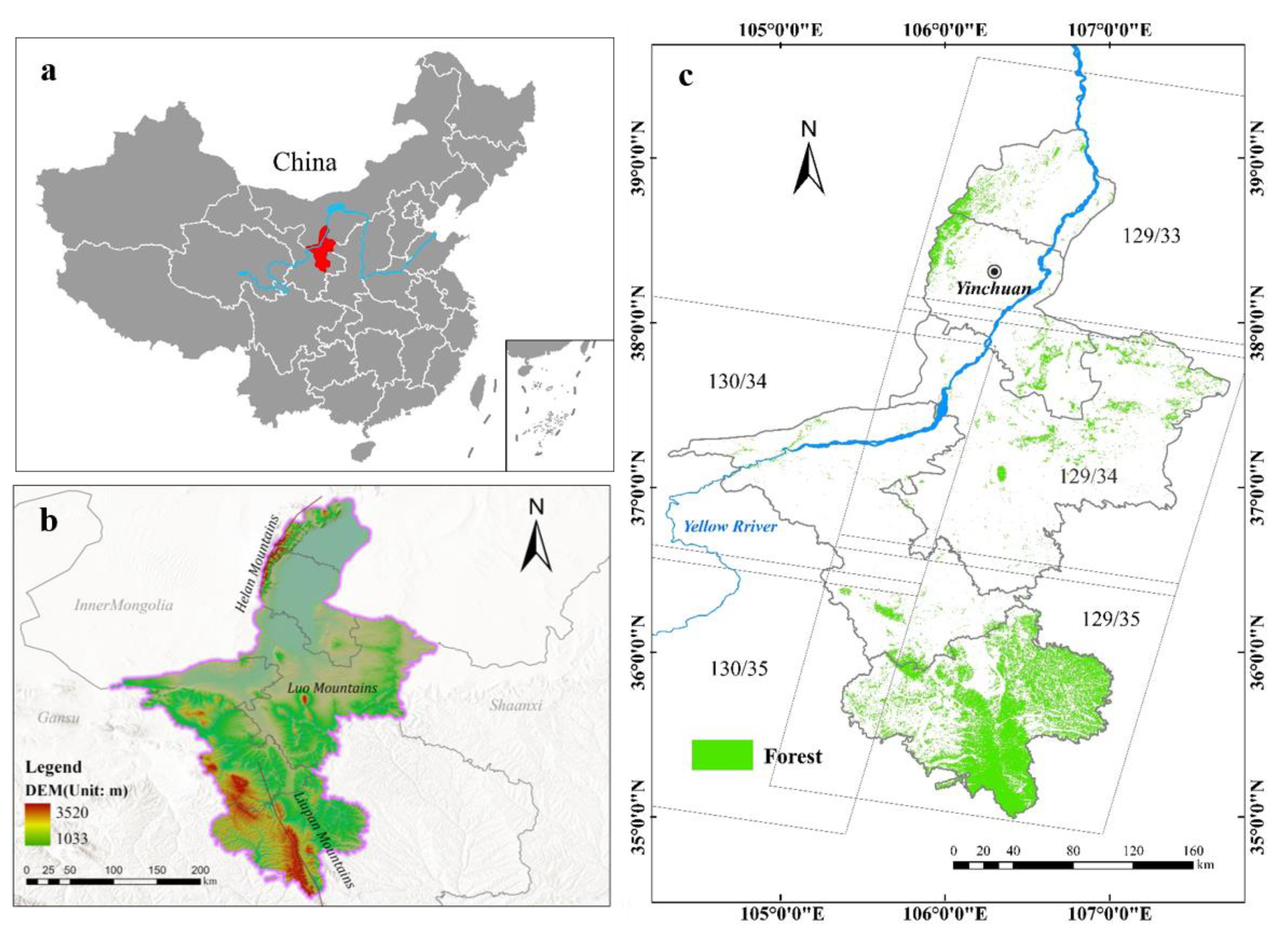
Figure 1. Location of the study area: (a) general location in China; (b) digital elevation model (DEM) of the study area; and (c) forest area of Ningxia Hui Autonomous Region in 2020.
Remotesensing 14 06188 g001
Figure 2. Workflow of the procedures developed in this study to map the planted forest dynamics. The major module is the OASB method, comprised two components: (1) image segmentation to yield forest objects and (2) a time-series classification to identify planted forests and estimate the planting year.
Remotesensing 14 06188 g002
Figure 3. Number of Landsat-5 TM, Landsat-7 ETM+, and Landsat-8 OLI scenes analyzed in this study, available annually from 1991 to 2020.
Remotesensing 14 06188 g003
Figure 4. Sensitivity analysis of the scale parameter (size) measured by the area-weighted local variance (ALV), Moran’s I of layers (MIL), and weighted score (WS).
Remotesensing 14 06188 g004
Figure 5. Five typical cases of NDVI trajectory patterns of forest objects: (a) intact natural forest; (b) clouds and cloud-shadow noise; (c) recovered natural forest; (d) planted forest converted from cropland; and (e) planted forest established on bare land. Notes: For each case, the time series (red broken line) is stacked via the object-level NDVI mean values, whereas the range of values for the homogenous pixels is represented by the shadow area. The shapelet is composed of the time nodes covered by the blue area, and a statistic χ 2 calculated using the m-test explains the significance of the difference between the shapelet and non-shapelet.
Remotesensing 14 06188 g005
Figure 6. Frequency histogram of the χ 2 statistics of the m-test for all forest objects. With a threshold χ 2   = 7.88 at the significance level α = 0.005 , the histogram is divided into two parts: natural forest (dark green bars) and planted forest (light green bars).
Remotesensing 14 06188 g006
Figure 7. NDVI time-series (top) and Landsat imagery cutouts (bottom) of a planted forest sample. The top part of the figure is the NDVI time series (1990–2020) of the sample; the bottom part consists of 8 Landsat composite images from different years to depict the variation in the spectral reflectance of the sample during the period of study, and the location of the sample is indicated by a yellow polygon in the center of each image. The planting year of the sample in 2003 can be inferred.
Remotesensing 14 06188 g007
Figure 8. (a) SNIC superpixels (white polygons) against the background of Landsat composite images in 1991, 2000, 2010, and 2020. (b) High-resolution images on Google Earth in 2009 (the earliest) and 2020 as reference data.
Remotesensing 14 06188 g008
Figure 9. (a) Map of the NHAR’s planted and natural forests in 2020. (b) The zoomed-in views of three regions corresponding to the labels 1, 2, and 3 in (a). (c) High-resolution images from Google Earth of the three regions. (df) Landsat images (in false color composite) in 1991, 2005, and 2020 of the three regions (9 images in total), respectively.
Remotesensing 14 06188 g009
Figure 10. (a) The 2020 NHAR planting year map. (bd) Enlarged maps of the three regions labeled as 1, 2, and 3 in (a). (e) Statistical data of the afforestation area for each year from official statistics (blue bars), and estimated data of the annual planting area derived from the planting year map (orange broken line).
Remotesensing 14 06188 g010
Figure 11. Comparison between the mapped and observed years of forest planting. The colorful dots simultaneously represent the two data sources for the planted forest sample, and the color represents the number of dots in the same position; the straight red line is the linear regression between the two data sources.
Remotesensing 14 06188 g011
Table 2. Confusion matrix of the NHAR natural/planted forest maps in 2020.
Land CoverClassified DataTotalProducer Accuracy (PA)
Natural ForestPlanted ForestNon-Forest
Referenced DataNatural forest892910089.0%
Planted forest2811710081.0%
Non-forest359210092.0%
Total9488118300
User Accuracy (UA)94.7%92.0%78.0%
Overall Accuracy = 87.3%, Kappa = 0.82.
Publisher’s Note: MDPI stays neutral with regard to jurisdictional claims in published maps and institutional affiliations.