Global Change of Land-Sparing and Land-Sharing Patterns over the Past 30 Years: Evidence from Remote Sensing and Statistics

Abstract

Agricultural expansion, driven by the increasing demand on crops, poses a severe threat to the global environment and to human welfare. Regarded as an effective landscape pattern for balancing biodiversity and food security, land sparing bears high expectations from ecologists. To reflect the spatial-temporal pattern change of land sparing, we calculate a land sparing/sharing (LSS) index on the basis of a remote sensing dataset. The land-sparing pattern has shown an apparent increasing trend globally, especially in hotspots, including the eastern United States, central South America, northern Europe, Kazakhstan, southeastern China, and the Korean Peninsula. Meanwhile, the land-sharing pattern has been increasing in some other regions, including in the southeast of South America, western Europe, central Europe, southern Europe, and northwestern China. However, according to statistical datasets, contrary to the overall increasing trend of land sparing, passive land sparing, incentivized by lower food prices due to increased yields, is decreasing, especially in countries with high levels of development. Our results reveal the global trends in land sparing and passive land sparing, providing support for balancing biodiversity conservation and food security among countries and ecoregions.

1. Introduction

A constantly growing global population and food demands have led to the expansion of agricultural lands and the loss of wild nature, which is a major threat to biodiversity, ecosystem services, as well as human health and well-being [1,2]. In order to achieve the United Nations Sustainable Development Goals, balancing food security and biodiversity conservation remains one of the greatest challenges in the 21st century [3]. The land-sharing versus land-sparing framework is widely used to address this issue [4]. The land-sharing pattern integrates land for nature and land for agriculture, so as to guarantee a partly win-win situation of biodiversity conservation and crop production, while the land-sparing pattern separates intensively used agricultural land from biodiversity conservation in order to spare more land for nature [5,6,7].

Many studies have conducted comparative analyses on land-sharing and land-sparing patterns, involving multiple aspects, including the food supply, spatial scale, environmental heterogeneity, and biodiversity conservation [6,8,9,10]. The land-sparing pattern has been considered as a possible solution to reducing the negative impacts of agricultural expansion [11], and is more beneficial to species that are sensitive to agriculture or that require a large range of space [12,13]. Increasing crop yields reduce the need to convert more wild nature into croplands to meet growing food demands, resulting in more intact habitats and facilitating biodiversity conservation [14,15]. The above studies supporting land sparing mainly focus on the pattern’s benefits to agricultural production, ecosystem services, and species protection in a certain region. However, little importance is attached to the spatial-temporal pattern change of land sparing. Pompeu et al. developed the land sharing/sparing index and used a 30-m resolution landcover map, on the basis of 2013 Landsat images, to analyze land-sparing patterns in the Cerrado, on the Brazilian Savanna [16]. Lin and Huang adopted annual agricultural statistics on the county scale from the USDA National Agricultural Statistics Service and visualized the relationship between the yields and the cropland area from 1974 to 2008, which was analyzed by bivariate regression [17]. Neither at a large spatial scale, nor in a long time series, are remote sensing and statistics combined. Besides active land sparing, which directly links increasing yields with habitat protection or restoration, there is another land-sparing pattern, namely, passive land sparing, whereby the clearance of agricultural lands is incentivized by lower food prices due to increased yields [18,19]. In the passive land-sparing pattern, there are rebound effects since the demands boosted by the decreased prices and profits expanded by increased yields can weaken the motivation for sparing land. Balmford et al. projected cropland-area change between 2000 and 2050, using trends extracted from statistical data, and concluded that a higher level of yield growth would demand less cropland area, even with a larger population [11]. Ewers et al. investigated the relationship between the per capita cropland area (PCCA) and the combined energy yield of 23 staple crops and found that wild nature had benefited from passive land sparing caused by increasing agricultural yields from 1979 to 1999 [20]. Nevertheless, how has this phenomenon changed over time? Is it strengthening or weakening? What does this mean for food production and biodiversity conservation? These issues still need further consideration.

Hence, we aim to uncover the spatial-temporal pattern of land sparing at the global scale, to identify hotspots for ecoregions, and to reveal the trend of passive land sparing for countries. On the basis of the European Space Agency Climate Change Initiative Land Cover (ESA-CCI LC) [21], we first calculated a land sparing/sharing index (LSS) from 1992 to 2018, and then obtained the change rate of LSS by linear regression at both the pixel scale and the ecoregion scale. Moreover, the influence of the landcover maps’ resolution on LSS is analyzed by comparing LSS calculated from a nominal 30-m annual land use/land cover dataset, (CLUD-A) 2015, for China [22,23], and the United States National Land Cover Database, (NLCD) 2016 [24,25,26], at different resolutions. Statistical data from the Food and Agriculture Organization Corporate Statistical Database (FAOSTAT) [27] is further incorporated in order to explore the relationship between the PCCA change and the yield change, so as to identify countries in the passive land-sparing pattern during the period from 1961 to 2018. Mapping the global spatial-temporal pattern of land sparing helps to identify hotspots of ecoregions and serves as a guideline for nature conservation in the light of local conditions. At the country scale, the passive land-sparing pattern’s weakening with the level of development-promoting has sounded the alarm, calling for more efforts to optimize the landscape pattern in order to balance biodiversity conservation and food security.

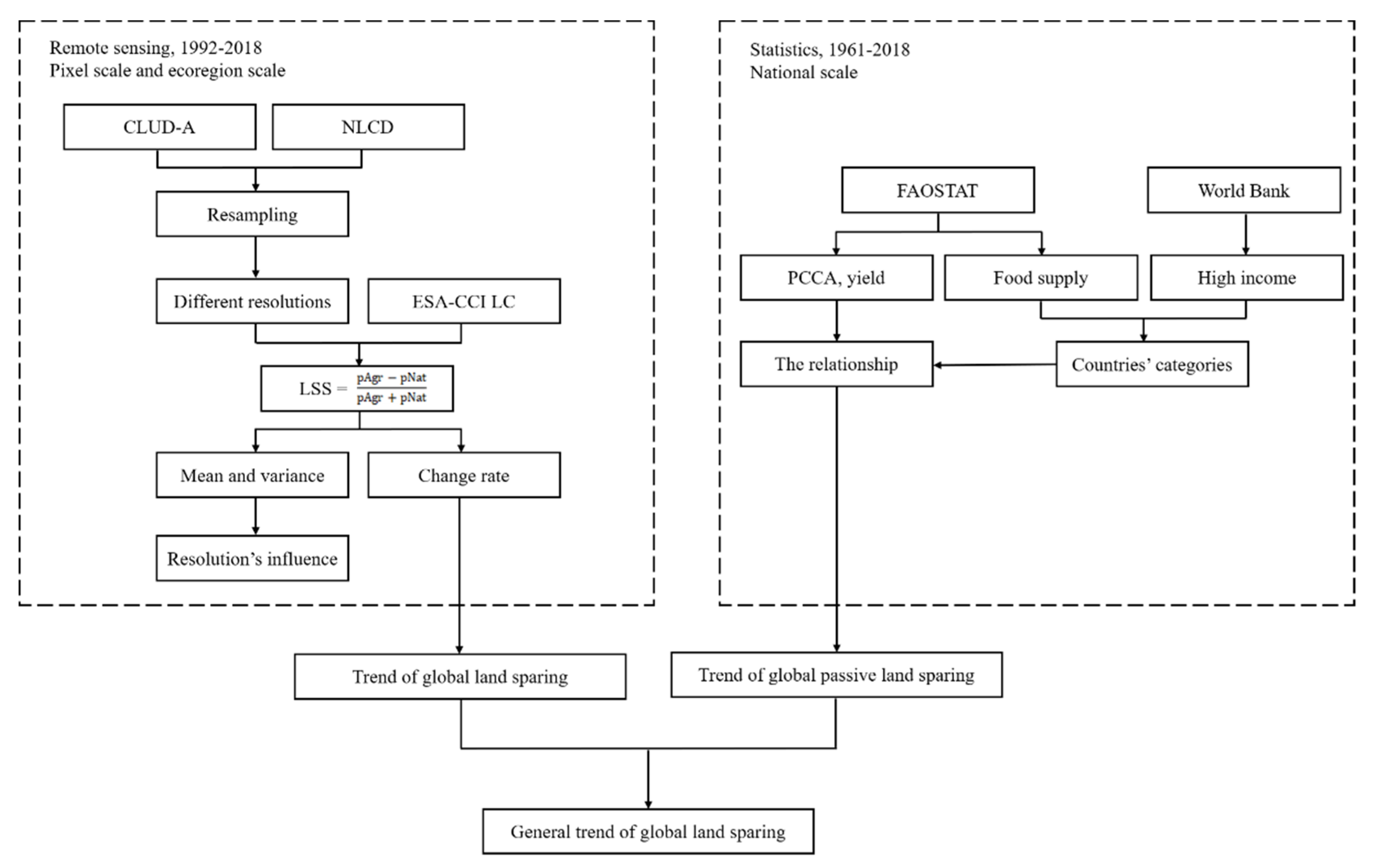
2. Materials and Methods

This study consists of two parts (Figure 1). The first part is based on remote sensing to identify land sparing at the pixel scale, including Section 2.1, Section 2.2, and Section 2.3, while the second part, which is illustrated in Section 2.4, adopts statistics to identify passive land sparing at the national scale. Since the active land-sparing pattern, which directly relates to yields increasing with conservation, is hard to monitor, we analyze the general trend of the global land-sparing pattern by identifying trends of both land sparing and passive land sparing.

In the first part, we use the ESA-CCI LC to calculate global LSS (Section 2.1) and explore its change rate at the pixel scale and the ecoregional scale (Section 2.2) so as to identify the trend of the land-sparing pattern from 1992 to 2018. Moreover, we introduce CLUD-A 2015 and NLCD 2016 to analyze the resolution’s influence on LSS (Section 2.3). In the second part, on the basis of statistical data from FAOSTAT, the passive land-sparing pattern from 1961 to 2018, which is reflected by the relationship between the PCCA and the yield, is identified at the national scale (Section 2.4).

2.1. Calculation of LSS Based on ESA

The land sharing/sparing index was proposed as Equation (1) to reflect the land-sparing/-sharing patterns in a certain region [16]. This index is based on the idea that the land-sparing pattern and the land-sharing pattern are opposite endpoints of a continuum of separation between biodiversity and agriculture [5].

$$\mathrm{Land} \mathrm{Sharing}/\mathrm{Sparing} \mathrm{Index}=\frac{\mathrm{pNat}-\mathrm{pAgr}}{\mathrm{pNat}+\mathrm{pAgr}},$$

(1)

We develop an inverse index, named the LSS index, to focus on the land-sparing pattern. The LSS index is calculated at the pixel scale, as shown in Equation (2). In an agricultural landscape at a certain scale, the land-sharing pattern exhibits substantial natural patches and some agricultural patches, while the land-sparing pattern represents agriculture’s dominance over nature in the aspect of an area. Thus, the maximum of the natural area ratio could stand for the land-sharing endpoint, while the natural area ratios approaching 0 could stand for the land-sparing endpoint [16].

$$\mathrm{Land} \mathrm{Sparing}/\mathrm{Sharing} \mathrm{Index}=\frac{\mathrm{pAgr}-\mathrm{pNat}}{\mathrm{pAgr}+\mathrm{pNat}},$$

(2)

where pAgr is the area proportion of the agricultural classes, and pNat is the area proportion of the natural classes. This index ranges, theoretically, from −1 to 1, separately representing nature’s occupation of almost the whole pixel, and the opposite situation, the agricultural area’s dominance over natural area. Hence, a positive LSS value represents a land-sparing pattern, while a negative LSS value represents a land-sharing pattern. The greater the LSS value, the stronger the trend of the land-sparing pattern.

The calculation of the LSS index is based on the global ESA-CCI LC, which is a time series of consistent global LC maps, with a 300-m spatial resolution, from 1992 to 2018 [28]. This dataset is generated using multiyear and multisensor strategies to utilize all appropriate data and maximize product consistency. On the basis of the Land Cover Classification System developed by the Food and Agriculture Organization of the United Nations (FAO), the ESA-CCI LC contains 37 types (classes) of original land cover, with an overall accuracy of approximately 71.1% [21].

In order to calculate the pNat and the pAgr, we reclassified the original ESA-CCI LC types. Urban areas (type 190), water bodies (type 210), and permanent snow and ice (type 220) were not considered. On one side, we merged rain-fed cropland (type 10), herbaceous cover (type 11), tree or shrub cover (type 12), and irrigated cropland (type 20) into the agricultural class. On the other side, there were 28 ESA-CCI LC types reclassified into the natural class, including different kinds of vegetation (types: 50, 60, 61, 62, 70, 71, 72, 80, 81, 82, 90, 100, 110, 120, 121, 122, 140, 150, 151, 152, 153, 160, 170, 180, 130, and 200) and bare areas (types 201 and 202). Especially for the mosaic types of the ESA-CCI LC, we assume that 60% and 40% of type 30 (mosaic where cropland (>50%)/natural vegetation (tree, shrub, herbaceous cover) (<50%)) is respectively occupied by agriculture and nature, while 40% and 60% of type 40 (mosaic where natural vegetation (tree, shrub, herbaceous cover) (>50%)/cropland (<50%)) is respectively occupied by agriculture and nature [29]. Finally, on the basis of the natural class and mosaic types, we count the number of pixels occupied by nature within a window of 10 km × 10 km, which is then multiplied by the actual area of each pixel (that is, 300 m × 300 m). The obtained product is the area of natural lands within 100 km² and a pNat with a resolution of 10 km is further calculated. Similarly, we count the number of pixels covered by agriculture, according to the agricultural class and mosaic types, and calculate the gridded pAgr. The annual global LSS maps from 1992 to 2018 are then derived from the pNat and the pAgr.

2.2. Exploration of LSS Change Rate at Pixel Scale and Ecoregion Scale

We implemented linear regression to obtain the change rates of the global LSS over the period from 1992 to 2018. The change rates and the corresponding p-values were calculated at a pixel scale. For pixels whose p-values were greater than or equal to 0.05, that is, those who failed to pass the significance test, the change rates were regarded as invalid.

We further explored the change of LSS at the ecoregional scale. There are 867 terrestrial ecoregions, where unique natural communities are distributed and distinct species are inhabited, belonging to 14 different biomes [30]. On the basis of the valid change rate of global LSS at the pixel scale, the mean change rate of LSS for terrestrial ecoregions is calculated, which facilitates the identification of hotspots for landscape pattern change.

2.3. Analyses of Resolution’s Influence on LSS

We were concerned whether the 300-m resolution of the ESA-CCI LC would influence the LSS. In order to test the influence of the resolution on the LSS, we introduced 30-m resolution land-cover/land-use maps, respectively, for China and the Conterminous United States, that is, CLUD-A 2015 and NLCD 2016. The cropland area of China and the cropland area of the United States are both amongst the highest in the world. While the cropland in the United States basically occupies contiguous large areas, the cropland in China is mainly distributed in the plains and low hills of the central and eastern regions, showing a scattered spatial pattern in general. Hence, we selected these two typical countries with distinct cropland distributions to analyze the resolution’s influence on LSS.

The CLUD-A integrates an advanced very-high-resolution radiometer (AVHRR), a moderate-resolution imaging spectroradiometer (MODIS), and Landsat data, and provided nominal 30-m land use/land cover maps annually for China, from 1980 to 2015, with a classification system containing 11 classes [22,23]. On the basis of nearest neighbor interpolation, we resampled the CLUD-A 2015 from 30 m to 50 m, 100 m, 500 m, and 1000 m. The 10-km resolution LSS was calculated separately from the CLUD-A 2015 of the above five resolutions. Then we obtained the variance among all five LSS maps and the mean value of each LSS map. While calculating the LSS from the CLUD-A 2015, the agricultural class contains cropland (type 10), and the natural class includes vegetation (types 20, 30, and 40), wetland (type 50), and bare land (types 98 and 99). Waters (type 60), built-up (types 88 and 89) and snow/ice (type 100), were not taken into account.

Th Landsat-based NLCD maps the nationwide landcover for the Conterminous United States at a 30-m resolution, and contains 16 types, on the ground, of a modified Anderson Level II classification system [24,25,26]. Similar to the CLUD-A 2015, the NLCD 2016 was resampled to 50 m, 100 m, 500 m, and 1000 m by nearest neighbor interpolation. Furthermore, we calculated the 10-km LSS, from the NLCD 2016, of different resolutions and analyzed the difference. While calculating the LSS from the NLCD 2016, hay/pasture (type 81) and cultivated crops (type 82) are merged into the agricultural class to calculate the pAgr, while 8 types, including barren land (type 31), vegetation (types: 41, 42, 43, 52 and 71), and wetland (types: 90 and 95), are merged into the natural class to calculate the pNat. Open water (type 11), perennial snow/ice (type 12), and developed areas with different intensities (types 21, 22, 23, and 24) were not considered in the calculation of the LSS.

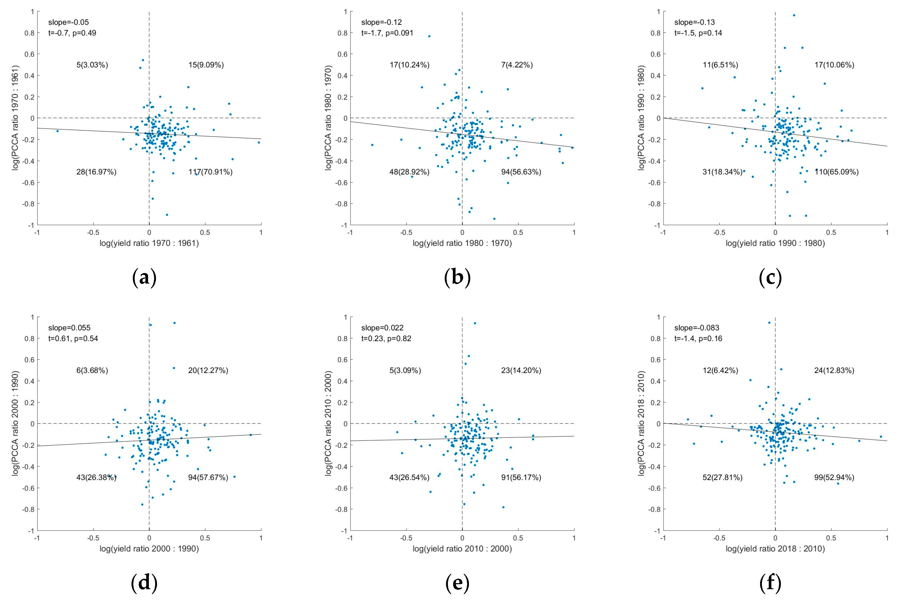
2.4. Exploration of the Relationship between the PCCA Change and the Yield Change

We explored the relationship between the PCCA change and the yield change using agricultural statistical data from FAOSTAT [27]. The statistical data is available at a country scale from 1961 to 2018, including the yields, arable land area, population, and food supply. We utilized statistical data from 1961, 1970, 1980, 1990, 2000, 2010, and 2018, focusing on six periods: 1961–1970, 1970–1980, 1980–1990, 1990–2000, 2000–2010, and 2010–2018.

Following the methodology of Ewers et al. [20], we assume that the change in the PCCA is negatively related to the change in the yield when land sparing occurs. At first, with reference to Balmford et al., we integrated the yield of the world’s 23 most energetically important food crops, which comprise all the world’s staple foods and which accounted for 60% of the global total harvested tonnage in 2000 [11], including bananas, barley, cassava, coconuts, grapes, groundnuts (with shell), maize, millet, oats, oil palm fruit, onions (dry), plantains and others, potatoes, paddy rice, sorghum, soybeans, sugar beet, sugar cane, sunflower seed, sweet potatoes, vegetables, wheat, and yams. The sum of the above 23 crop yields is used as the total food crop yield for each country. Then we calculated the PCCA at a country scale, in light of the FAOSTAT arable land area and the population data. Subsequently, countries were assigned to one of four categories to represent the different levels of development: low, medium-low, medium-high, and high. Countries defined as high-income countries by the World Bank [31] were assigned to the high category. The remaining countries were assigned to the low, medium-low, and medium-high categories, in the ascending order of the FAO food supply data of the first year during the period. The number of countries belonging to each category is approximately the same.

Finally, we analyzed the changes of the PCCA and the changes of the yields during each of the six time periods. For each period, we calculated each country’s yield ratio between the last year (e.g., 1970 for the 1961–1970 period) and the first year (e.g., 1961 for the 1961–1970 period). The logarithm of this ratio was used as the independent variable. The positive values of the independent variable mean yield increased, while the negative values of the independent variable mean yield decreased. Similarly, for each period, we calculated each country’s PCCA ratio between the last year and the first year. The logarithm of this ratio was used as the dependent variable. The positive values of the dependent variable mean PCCA increased, while the negative values of the dependent variable mean PCCA decreased. Additionally, two types of countries were excluded in the analysis: countries with absent data; and countries whose dependent or independent variables were extremely large or small, that is to say, they were situated outside the intervals [−1, 1].

3. Results

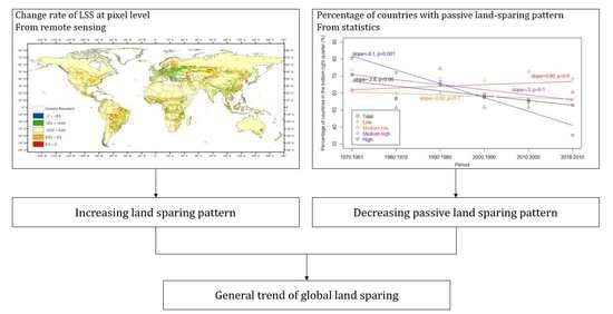
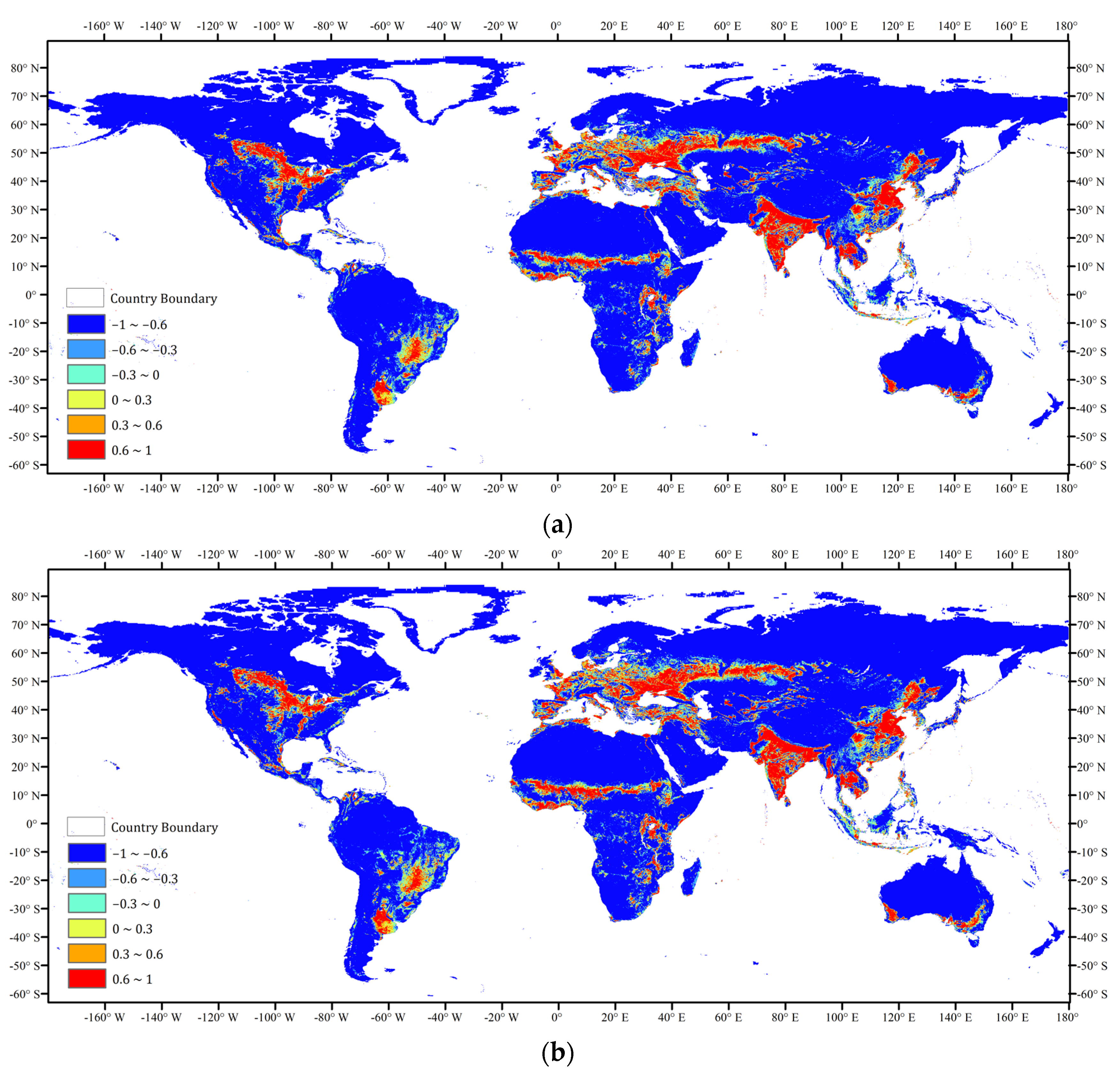
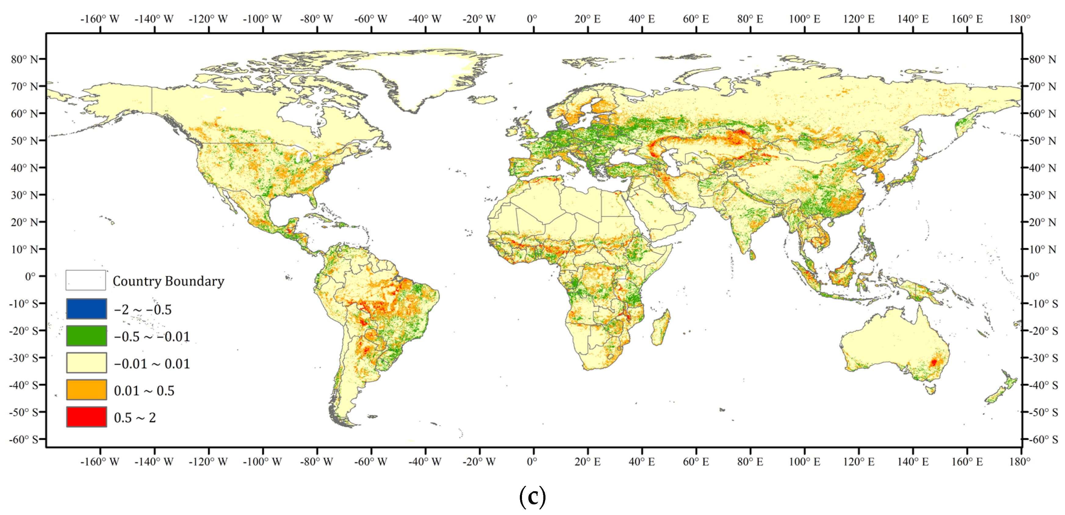
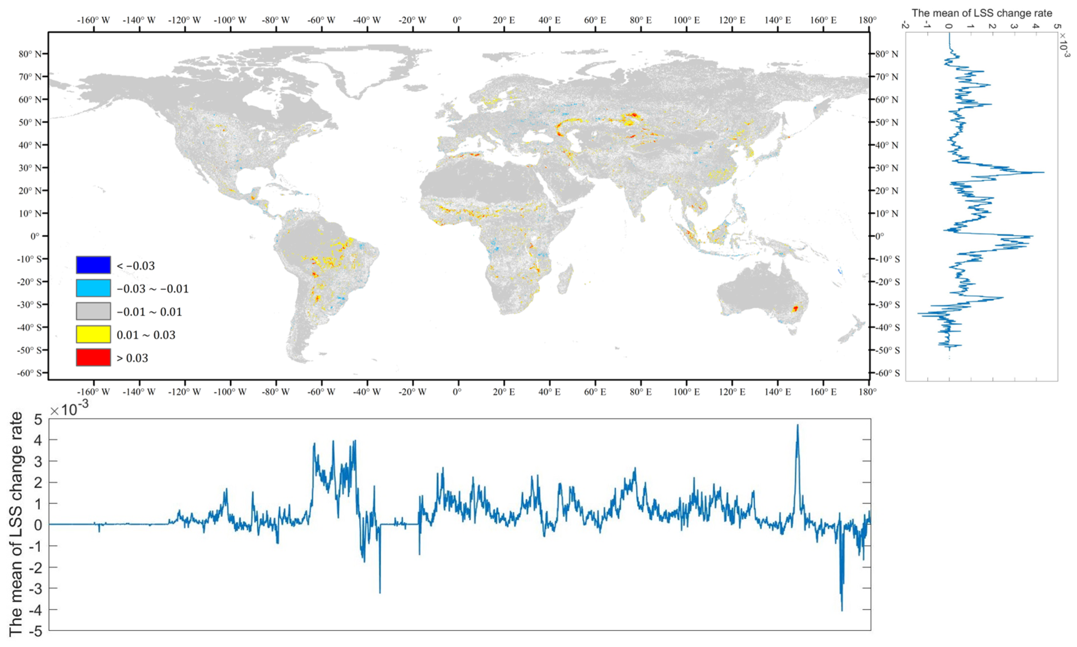
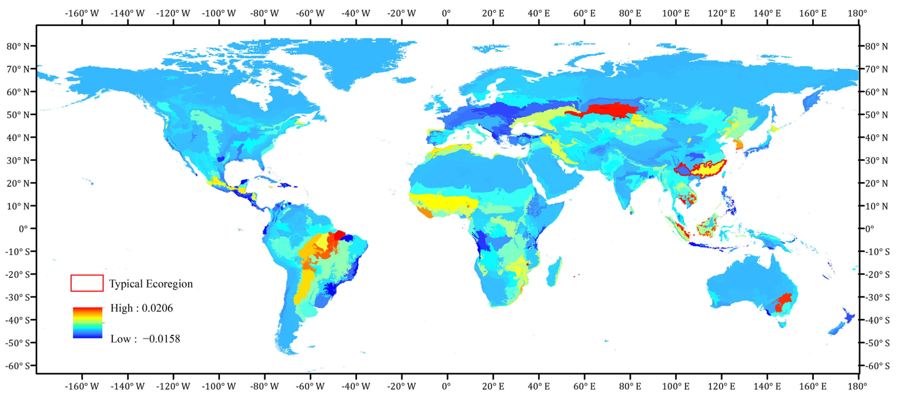
3.1. Trend of Land-Sparing Pattern in Global Cropland

Areas showing an intense land-sparing pattern have high values of LSS, which are mainly distributed in southern Canada, the United States Midwest, southern Brazil, eastern Argentina, central and east Africa, the whole of Europe, with the exception of northern Europe, India, China, Southeast Asia, and southeastern and southwestern Australia (Figure 2a,b). Compared with 1992, the land-sparing pattern in 2018 represents obvious expansion and intensification globally, especially in the eastern United States, central South America, northern Europe, Kazakhstan, southeastern China, and on the Korean Peninsula (Figure 2c). Yet some regions exhibit decreasing LSS, including the southeast of South America, western Europe, central Europe, southern Europe, and southwestern China, while others have kept approximately unchanged LSS, including nearly the whole of Australia, western China, southern Mongolia, western Asia, the Sahara Desert, northern Canada, and the state of Alaska.

The positive values of the LSS change rate mean an increasing land-sharing pattern, while the negative values of the LSS change rate mean a decreasing land-sharing pattern, over the period from 1992 to 2018. The mean LSS change rates of almost all longitudes and latitudes exhibit positive values, revealing the worldwide strengthening of land sparing since 1992 (Figure 3). This trend results from cropland intensification and expansion, and the development of sustainable intensive agriculture and increasing yields [18,32,33,34]. Only at around 35° and 45°W (eastern Brazil), 170°E (New Zealand and Kamchatka Peninsula), and 40–45°S (Uruguay and southeast Brazil) does the land-sparing pattern show a tendency toward decreasing, which is consistent with the result in Figure 2c.

At an ecoregional scale, most areas of the world have a positive LSS change rate, reflecting a strengthened land-sparing pattern and a weakening land-sharing pattern, which is related to, not only the factors mentioned before, but also to urban expansion, deforestation, and desertification [35,36,37] (Figure 4). There are 62 ecoregions identified as hotspots for increasing land sparing, whose LSS change rates are greater than 0.003 (Table S1). Meanwhile, there are 84 ecoregions identified as hotspots for decreasing land sparing, whose LSS change rates are less than −0.001 (Table S2). Among ecoregions covering relatively large areas, few have negative LSS values, such as Araucaria moist forests, the Uruguayan savanna, the Western Congolian forest-savanna mosaic, Western European broadleaf forests, Central European mixed forests, the Eastern European forest steppe, Chhota-Nagpur dry deciduous forests, Daba Mountains evergreen forests, and Yunnan Plateau subtropical evergreen forests, which are mainly located in Central America, in the southeast of South America, and in the southwests of Africa, Europe, India, and China. The tendency toward expanding the land-sparing pattern is obvious in central South America (e.g., the Tocantins/Pindare moist forests, the Mato Grosso seasonal forests, and the Madeira-Tapajós moist forests), West Africa (e.g., the West Sudan savanna, the Guinean forest-savanna mosaic), southeastern Africa (e.g., the Zambezian and Mopane woodlands, the Southern Miombo woodlands), Central Asia (e.g., the Kazakh steppe), East Asia (e.g., the Jiang Nan subtropical evergreen forests, Central Korean deciduous forests), and Southeast Asia (e.g., Southeastern Indochina dry evergreen forests, Sumatran peat swamp forests).

In order to analyze the factors influencing the landscape patterns of the ecoregions, we picked the Jiang Nan subtropical evergreen forests, with an intensifying land-sparing pattern, and the Yunnan Plateau subtropical evergreen forests, with a weakening land-sparing pattern, as typical ecoregions, which are bordered with red in Figure 4. This is because these two ecoregions are contiguous, and both have critical/endangered status but present the absolute opposite trend of the land-sparing pattern.

The Jiang Nan subtropical evergreen forests lie in southeastern China, extending from China’s southeast coast, westward to the Yunnan-Guizhou Plateau [38]. China exhibits apparent cropland intensification, and sufficient rainfall and heat provide the basis for the distribution of concentrated cropland in southern China [33]. Since rapid urbanization hinders future cropland expansion, and even threatens food security [35,39], cropland intensification becomes an effective alternative for maintaining agricultural production [40]. Moreover, the global deforestation map, based on the Landsat images, reveals wide forest losses in this ecoregion [36]. Therefore, deforestation and intensified agriculture facilitate the land-sparing pattern and further contribute to the increasing LSS in Figure 5a–d,i).

The Yunnan Plateau subtropical evergreen forests, located in southwestern China, provide habitat for endemic birds and support threatened species, such as Asiatic black bears and black gibbons, owning high values for biodiversity [41]. Initiated in 1999, China’s Grain for Green Programme motivates rural households by payment to convert arable land on steep slopes to forests, shrubs, and grassland [42], and has obvious effects on the promotion of forest restoration and vegetation coverage in Sichuan province and Yunnan province, where most of the area of the Yunnan Plateau subtropical evergreen forests lie [42,43]. Hence, raising restored forests benefits nature conservation in this ecoregion and undermines the land-sparing pattern, with LSS gradually decreasing from 1992 to 2018 (Figure 5e–h,j).

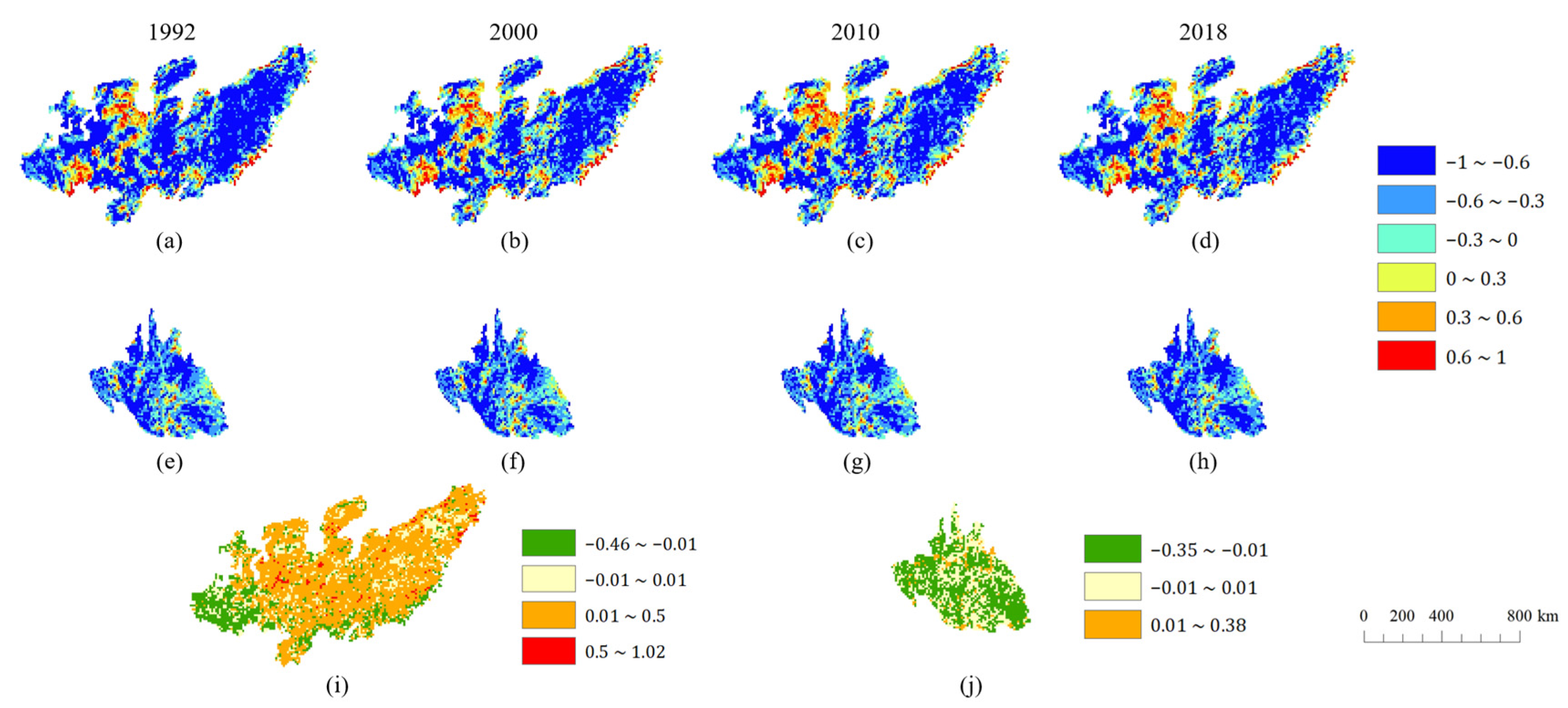
3.2. Influence of Resolution on LSS

To analyze the influence of resolution on the LSS, we resampled the CLUD-A 2015 by nearest neighbor interpolation and obtained five LSS maps of China at different resolutions. We calculated the nationwide LSS at a 10-km resolution from the CLUD-A 2015, at different resolutions of 30 m, 50 m, 100 m, 500 m, and 1000 m. At a pixel scale, we calculated the variance among the LSS maps calculated from the CLUD-A 2015 at different resolutions, and further obtained the area proportions within different variance ranges for China. At the national scale, we calculated the mean value of each LSS map. The processing of the NLCD 2016 for the Conterminous United States is consistent with that of the CLUD-A 2015 for China.

Apparently, most pixel variation is smaller than 0.05, and the area proportion of these pixels is 99.924% for China, and 99.920% for the Conterminous United States (

Table 1. Area proportions within different variance ranges for China and the Conterminous United States (abbreviated as “the US” in the table) (%).

Variance Range of China	Area Proportion of China	Variance Range of the US	Area Proportion of the US
[0, 0.005)	98.413	[0, 0.005)	97.542
[0.005, 0.01)	1.135	[0.005, 0.01)	1.767
[0.01, 0.05)	0.376	[0.01, 0.05)	0.611
[0.05, 0.1)	0.035	[0.05, 0.1)	0.045
[0.1, 0.5)	0.039	[0.1, 0.5)	0.029
[0.5, 0.58]	0.002	[0.5, 0.76]	0.006

). As for the mean value of the nationwide LSS, there is merely a faint difference among different resolutions, with a variance of 1.15 × 10⁻⁷ for China, and a variance of 3.63 × 10⁻⁷ for the Conterminous United States (

Table 2. Mean LSS for China and the Conterminous United States (abbreviated as “the US” in the table) from maps at different resolutions).

Resolution	Mean LSS of China	Mean LSS of the US
30 m	−0.58331	−0.49500
50 m	−0.58330	−0.49499
100 m	−0.58327	−0.49488
500 m	−0.58290	−0.49422
1000 m	−0.58255	−0.49364

). It is reliable that the resolution of the LC map has a relatively faint influence on the LSS. Therefore, the LSS calculated from the ESA-CCI LC of a 300-m resolution is stable and can accurately reflect global landscape patterns.

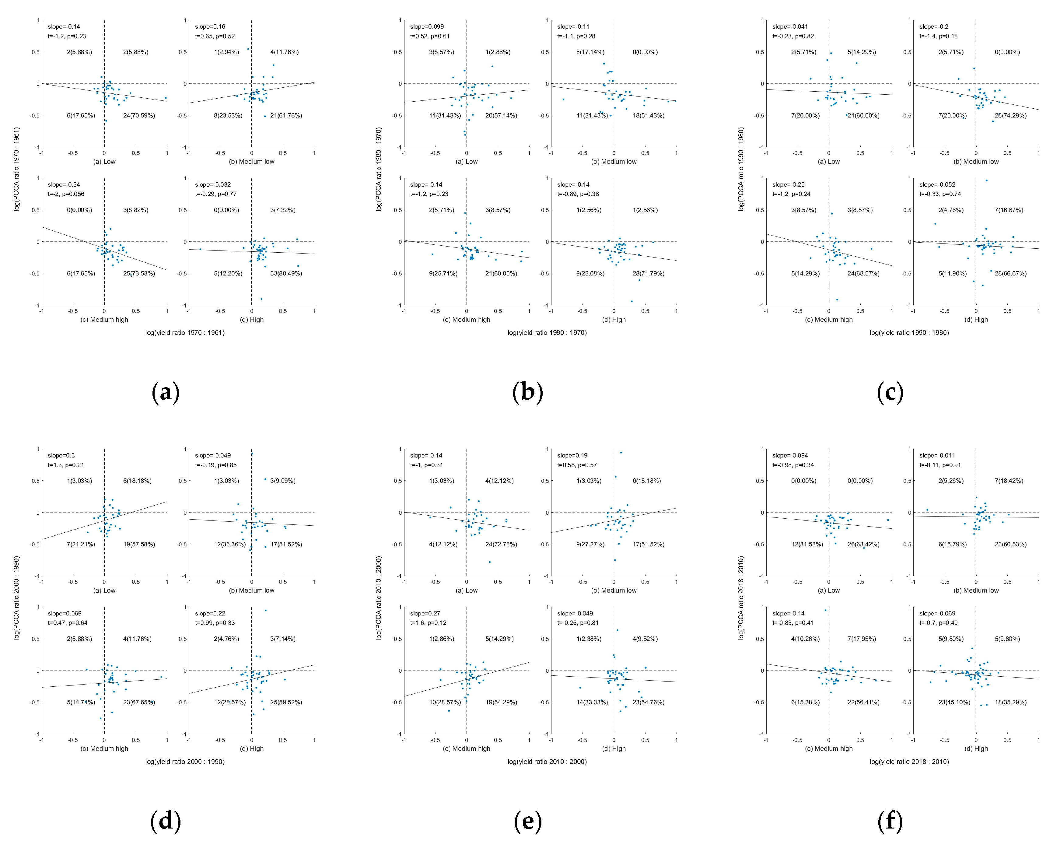
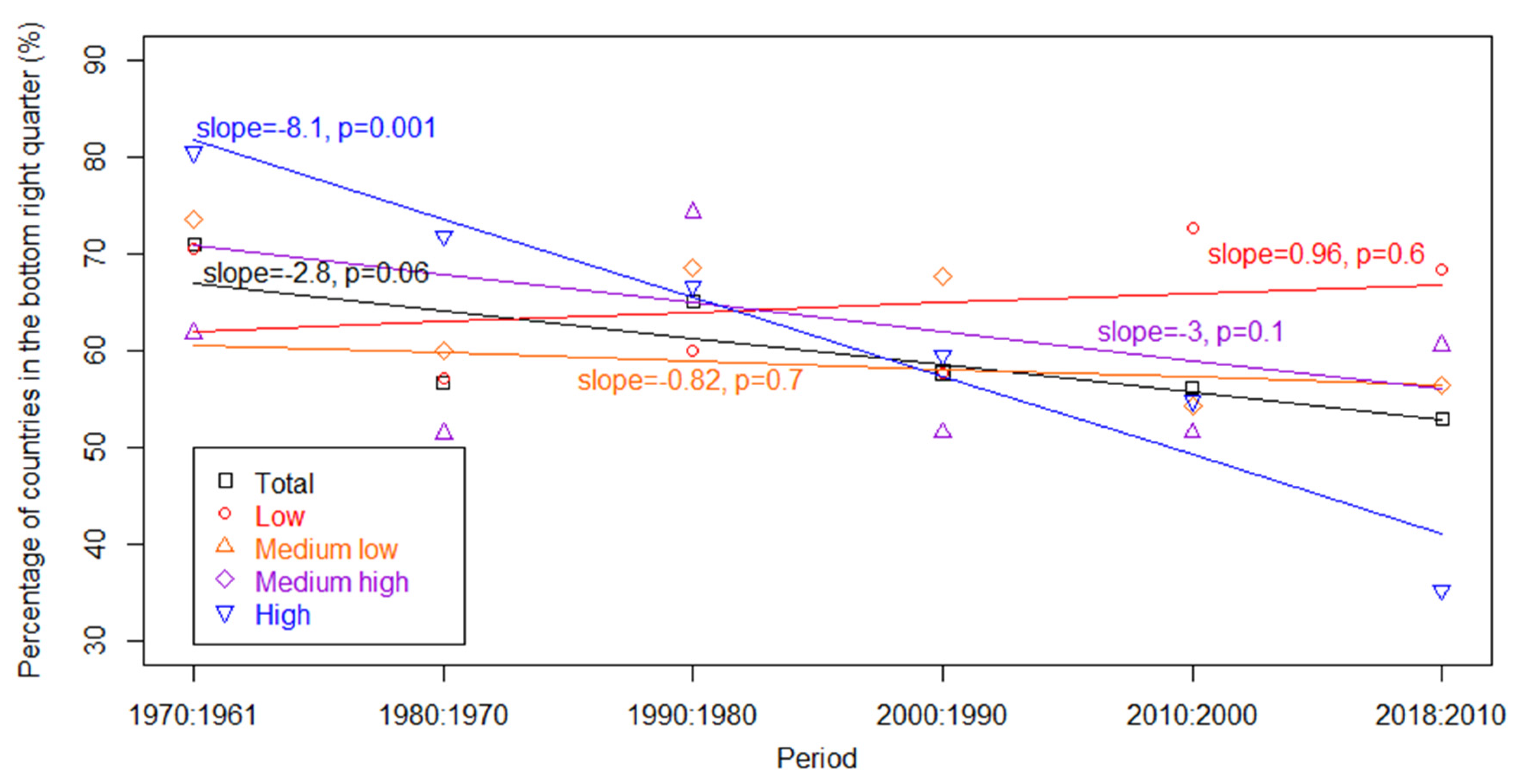
3.3. Effects of Passive Land Sparing on Countries

Figure 6 shows the relationship between the PCCA change and the yield change for all countries without classification. By contrast, Figure 7 separately depicts the relationship between the PCCA change and the yield change for four categories of countries. The countries in Figure 7 are assigned into four categories on the basis of the World Bank’s definition for high-income countries and FAOSTAT food supply data, including low, medium-low, medium-high, and high.

Countries with simultaneously increasing yields and decreasing PCCA are identified as belonging to the passive land-sparing pattern [20]. Hence, countries in the passive land-sparing pattern are located in the bottom right quarter, where the yield ratio is positive, and the PCCA ratio is negative (Figure 6 and Figure 7). As shown in Figure 6, during all six time periods, more than 50% of countries are in the passive land-sparing pattern, and the percentage is relatively high from 1961–1970 (70.91%), and from 1980–1990 (65.09%). Similarly, for the low, medium-low, and medium-high countries, the percentage of countries in the bottom right quarter ranges from 50 to 75% during different time periods (Figure 7). However, for high countries, the percentage presents an intense twist, decreasing from an amazingly high number of 80.49% for 1961–1970, to a surprising low number of 35.29% for 2010–2018.

The percentages of countries located in the bottom right quarter during different periods are illustrated in Figure 8. There is an obvious decreasing trend for all medium-low, medium-high, and high countries in the passive land-sparing pattern from 1961 to 2018. In this case, cropland will still expand extensively to meet food demands, despite simultaneously increasing yields, ratcheting up the risk of habitat destruction. On the basis of the slope fitted by linear regression, the intensity of the countries’ passive land-sparing decline in number is: high > medium-high > medium-low. For low countries, the percentage of countries in the passive land-sparing pattern presents an increasing trend. Hence, with the levels of development in the regions improving, passive land sparing derived from increasing yields presents a sign of abatement.

4. Discussion

According to the first draft of the post-2020 Global Biodiversity Framework [44], the first one of the 2030 action targets emphasizes integrated biodiversity-inclusive spatial planning to address land-use change. Agricultural land change has become the main form of land-use change, and agriculture covers about 38% of the Earth’s ice-free terrestrial area [45]. Cropland expansion and intensification lead to the loss, fragmentation, and degradation of natural habitats [46], and may continue to be the main driving force of biodiversity loss in the 21st century [47,48,49]. Hence, analyzing agricultural land patterns is of great significance to biodiversity conservation. In this study, we focus on the land-sparing pattern, an agricultural land pattern that represents higher crop yields, helps to meet food demands, and subsequently curbs agricultural encroachment on natural habitats.

It is necessary to understand the global trends of land sparing. For this reason, we have applied the LSS index, a basic index that reflects land-sparing patterns on a global scale. Identifying its trend is helpful for monitoring biodiversity from the perspective of land use. Remote sensing, which is characterized by a long time series and a large scale, provides a solid foundation for monitoring land-sparing patterns, continuously and globally. The LSS calculated from the remote sensing dataset, ESA-CCI LC, enables us to explore the trends in the land-sparing pattern at fine scales, such as at the pixel and ecoregional scales. Meanwhile, statistical data from FAOSTAT is incorporated to analyze the relationship between the yields and the PCCA at the national scale, reflecting the passive land-sparing pattern. Combining the trends of both land sparing and passive land sparing, we identify the general trend of land sparing and find that the effect of increasing yields on land sparing has been gradually weakening, highlighting that better organized and more effective measures of biodiversity management should be applied, especially in regions with apparent weakening trends.

Lin and Huang focused on the U.S. Midwest during the period from 1974–2008, at the county scale, and found that Kansas had an evident land-sparing pattern, while Minnesota and South Dakota had weakening land-sparing patterns, which, to some extent, corresponds to the increased LSS from 1992 to 2018 in these two states (Figure 2c) [17]. Considering the distinct research periods (1992–2018 versus 1974–2008), the data sources (remote sensing versus statistics), and the spatial scales (pixel versus county) between this study and Lin and Huang’s, it is hard to make a more detailed comparison or identify subtler differences. Ewers et al. identified a faint decreasing trend of PCCAs with yields, increasing in developing countries, while there is no obvious association between PCCAs and yields in developed countries from 1979 to 1999 [20]. On the basis of the statistical data, we conclude that countries of the low category show marked passive land-sparing trends from 1961 to 2018, which is consistent with Ewers et al. Meanwhile, land-sparing patterns are weakening among countries of the other three categories, and the weakening intensity is strengthening in the ascending order of the medium-low, medium-high, and high categories, which differs from the trend of 1979–1999, and is possibly related to the prevalence of agricultural subsidies, as well as to technical limitations.

With regard to the LSS index, there are some deficiencies to be improved in future studies.

First of all, the land sharing/sparing index has been used to identify land-sparing patterns at the landscape scale [16]. On the basis of the former study, we develop the LSS index and explore a global application of this index. It should be recognized that the LSS index, as a basic index reflecting land-use change, exhibits the overall pattern of land sparing, and more detailed analyses in the future need to be combined with regional biodiversity data. The LSS index concentrates on the extent to which more land is spared, since the spared land is possibly of benefit to natural habitats. However, the LSS monitors the condition of biodiversity conservation indirectly, on the basis of the hypothesis that the strengthening of land sparing indicates more secured habitats. Areas of conserved habitats are not included directly in the LSS index. This may cause an overestimation of the land sparing’s positive effects on biodiversity, considering that some spared cropland could be kept bare, or could be exploited for other human uses, such as urbanization [50]. Further improvement of the LSS index could combine indicators directly related to biodiversity, such as the area of the habitat secured.

Secondly, since the spatial-temporal pattern change of land sparing was identified on the basis of the remote sensing dataset, the results focus on the aspect of land use and take no account of cropping intensity, irrigation, and field management. Indeed, these ignored factors can be extremely beneficial to strengthening land sparing when appropriately addressed. Hence, the practical trend of land sparing could be stronger than the results indicate in this study.

Moreover, agricultural placement could be optimized by shifting crop production to regions with lower biodiversity and higher yield potentials, contributing greatly to the advancement of habitat and biodiversity conservation [51]. Thus, the spatial heterogeneity of the demand and the crop yield, which is not incorporated in the LSS index, requires more attention, and, to compensate for this, we introduced FAOSTAT statistics at the national scale, which provides corresponding information. Global socioeconomic data at finer spatial scales are difficult to obtain. The factors affecting the LSS index and the land-sparing pattern, such as deforestation and intensified agriculture, vary with the regions. The former does harm to nature conservation, while the latter may achieve sustainable development and help restore ecosystem services through appropriate implementation, such as impelling incentive mechanisms, promoting land and water management, and reclaiming salinized land [52,53]. Hence, more specific and detailed research, targeting distinct regions and ecoregions, is in demand. Overall, we have depicted the spatial-temporal pattern of land sparing, but whether to encourage or curb the strengthening of land sparing depends on the local conditions of regions. The scale and specific circumstances of the landscape (e.g., topography, climate, and productivity), socioeconomic factors (e.g., population density, financial inputs, technological adoption, and policies), endemic species richness, and the response of biodiversity to cropping intensity should all be considered when formulating policies for a certain region on a landscape pattern [5,6,54,55].

5. Conclusions

On the one hand, land sparing has been expanding widely all over the world in the past few decades, affecting both developing and developed countries. Most mean LSS change rates of longitudes and latitudes are positive, illustrating an increasing tendency toward the land-sparing pattern. However, the absolute values of the LSS change rate are relatively small at all four scales: pixel, longitude, latitude, and ecoregion. This demonstrates that the current trend of the global land-sparing pattern is faint, and that it has the potential of being changed by effective measures.

On the other hand, though increasing yields could benefit land sparing, this effect has been gradually weakening in most areas in past decades. We find that the land-sparing benefits of increasing yields decrease with the level of development of a region. This may be caused by complex and complicated reasons. For example, agricultural subsidies may distort land sparing by providing incentives for production beyond the needs of the human population [20], and there may be bottlenecks in yield improvement because of technical limitations [56,57].

While the specific situations of each country need to be further analyzed using national yield, cropland area, and population datasets, our results have demonstrated generally weakening trends of passive land sparing, indicating that more wild nature may be lost as a result of agricultural expansion. If this trend continues, nature conservation may face even more challenges in the future. Thus, further actions should be carried out to balance food security and nature conservation in the coming decades, including the careful consideration and implementation of active land-sparing strategies, such as land-use zoning, economic instruments (e.g., payments, land taxes, and subsidies), and the spatially strategic deployment of technology, infrastructure, or agronomic knowledge, and standards/certification [18].

References

1. Foley, J.A.; DeFries, R.; Asner, G.P.; Barford, C.; Bonan, G.; Carpenter, S.R.; Chapin, F.S.; Coe, M.T.; Daily, G.C.; Gibbs, H.K.; et al. Global Consequences of Land Use. Science 2005, 309, 570. [Google Scholar] [CrossRef] [Green Version]
2. Kehoe, L.; Romero-Muñoz, A.; Polaina, E.; Estes, L.; Kreft, H.; Kuemmerle, T. Biodiversity at risk under future cropland expansion and intensification. Nat. Ecol. Evol. 2017, 1, 1129–1135. [Google Scholar] [CrossRef] [PubMed]
3. Tscharntke, T.; Clough, Y.; Wanger, T.C.; Jackson, L.; Motzke, I.; Perfecto, I.; Vandermeer, J.; Whitbread, A. Global food security, biodiversity conservation and the future of agricultural intensification. Biol. Conserv. 2012, 151, 53–59. [Google Scholar] [CrossRef]
4. Fischer, J.; Abson, D.J.; Butsic, V.; Chappell, M.J.; Ekroos, J.; Hanspach, J.; Kuemmerle, T.; Smith, H.G.; von Wehrden, H. Land Sparing Versus Land Sharing: Moving Forward. Conserv. Lett. 2014, 7, 149–157. [Google Scholar] [CrossRef] [Green Version]
5. Fischer, J.; Brosi, B.; Daily, G.C.; Ehrlich, P.R.; Goldman, R.; Goldstein, J.; Lindenmayer, D.B.; Manning, A.D.; Mooney, H.A.; Pejchar, L.; et al. Should agricultural policies encourage land sparing or wildlife-friendly farming? Front. Ecol. Environ. 2008, 6, 380–385. [Google Scholar] [CrossRef]
6. Phalan, B.; Onial, M.; Balmford, A.; Green, R.E. Reconciling Food Production and Biodiversity Conservation: Land Sharing and Land Sparing Compared. Science 2011, 333, 1289. [Google Scholar] [CrossRef]
7. Green, R.E.; Cornell, S.J.; Scharlemann, J.; Balmford, A. Farming and the fate of wild nature. Science 2005, 307, 550–555. [Google Scholar] [CrossRef] [PubMed] [Green Version]
8. Grau, R.; Kuemmerle, T.; Macchi, L. Beyond ‘land sparing versus land sharing’: Environmental heterogeneity, globalization and the balance between agricultural production and nature conservation. Curr. Opin. Environ. Sust. 2013, 5, 477–483. [Google Scholar] [CrossRef]
9. Jiang, G.; Wang, G.; Holyoak, M.; Yu, Q.; Jia, X.; Guan, Y.; Bao, H.; Hua, Y.; Zhang, M.; Ma, J. Land sharing and land sparing reveal social and ecological synergy in big cat conservation. Biol. Conserv. 2017, 211, 142–149. [Google Scholar] [CrossRef] [Green Version]
10. Mehrabi, Z.; Ellis, E.C.; Ramankutty, N. The challenge of feeding the world while conserving half the planet. Nat. Sustain. 2018, 1, 409–412. [Google Scholar] [CrossRef] [Green Version]
11. Balmford, A.; Green, R.E.; Scharlemann, J.P.W. Sparing land for nature: Exploring the potential impact of changes in agricultural yield on the area needed for crop production. Glob. Chang. Biol. 2005, 11, 1594–1605. [Google Scholar] [CrossRef]
12. Law, E.A.; Meijaard, E.; Bryan, B.A.; Mallawaarachchi, T.; Koh, L.P.; Wilson, K.A. Better land-use allocation outperforms land sparing and land sharing approaches to conservation in Central Kalimantan, Indonesia. Biol. Conserv. 2015, 186, 276–286. [Google Scholar] [CrossRef] [Green Version]
13. Crespin, S.J.; Simonetti, J.A. Reconciling farming and wild nature: Integrating human—Wildlife coexistence into the land-sharing and land-sparing framework. Ambio 2019, 48, 131–138. [Google Scholar] [CrossRef] [PubMed]
14. Balmford, A.; Amano, T.; Bartlett, H.; Chadwick, D.; Collins, A.; Edwards, D.; Field, R.; Garnsworthy, P.; Green, R.; Smith, P.; et al. The environmental costs and benefits of high-yield farming. Nat. Sustain. 2018, 1, 477–485. [Google Scholar] [CrossRef] [PubMed]
15. Garnett, T.; Appleby, M.C.; Balmford, A.; Bateman, I.J.; Benton, T.G.; Bloomer, P.; Burlingame, B.; Dawkins, M.; Dolan, L.; Fraser, D.; et al. Sustainable Intensification in Agriculture: Premises and Policies. Science 2013, 341, 33. [Google Scholar] [CrossRef]
16. Pompeu, J.; Soler, L.; Ometto, J. Modelling Land Sharing and Land Sparing Relationship with Rural Population in the Cerrado. Land 2018, 7, 88. [Google Scholar] [CrossRef] [Green Version]
17. Lin, M.; Huang, Q. Exploring the relationship between agricultural intensification and changes in cropland areas in the US. Agric. Ecosyst. Environ. 2019, 274, 33–40. [Google Scholar] [CrossRef]
18. Phalan, B.; Green, R.E.; Dicks, L.V.; Dotta, G.; Feniuk, C.; Lamb, A.; Strassburg, B.B.N.; Williams, D.R.; Ermgassen, E.K.H.J.; Balmford, A. How can higher-yield farming help to spare nature? Science 2016, 351, 450. [Google Scholar] [CrossRef] [PubMed] [Green Version]
19. Balmford, B.; Green, R.E.; Onial, M.; Phalan, B.; Balmford, A. How imperfect can land sparing be before land sharing is more favourable for wild species? J. Appl. Ecol. 2019, 56, 73–84. [Google Scholar] [CrossRef] [Green Version]
20. Ewers, R.M.; Scharlemann, J.P.W.; Balmford, A.; Green, R.E. Do increases in agricultural yield spare land for nature? Glob. Chang. Biol. 2009, 15, 1716–1726. [Google Scholar] [CrossRef]
21. Defourny, P.; Lamarche, C.; Bontemps, S.; De Maet, T.; Van Bogaert, E.; Moreau, I.; Brockmann, C.; Boettcher, M.; Kirches, G.; Wevers, J.; et al. Land Cover CCI: Product User Guide Version 2.0. Tech. Rep. 2017. Available online: Maps.elie.ucl.ac.be/CCI/viewer/download/ESACCI-LC-Ph2-PUGv2_2.0.pdf (accessed on 3 March 2021).
22. Liu, J.; Zhang, Z.; Xu, X.; Kuang, W.; Zhou, W.; Zhang, S.; Li, R.; Yan, C.; Yu, D.; Wu, S.; et al. Spatial patterns and driving forces of land use change in China during the early 21st century. J. Geogr. Sci. 2010, 20, 483–494. [Google Scholar] [CrossRef]
23. Xu, Y.; Yu, L.; Peng, D.; Zhao, J.; Cheng, Y.; Liu, X.; Li, W.; Meng, R.; Xu, X.; Gong, P. Annual 30-m land use/land cover maps of China for 1980–2015 from the integration of AVHRR, MODIS and Landsat data using the BFAST algorithm. Sci. China Earth Sci. 2020, 63, 1390–1407. [Google Scholar] [CrossRef]
24. Yang, L.; Jin, S.; Danielson, P.; Homer, C.; Gass, L.; Bender, S.M.; Case, A.; Costello, C.; Dewitz, J.; Fry, J.; et al. A new generation of the United States National Land Cover Database: Requirements, research priorities, design, and implementation strategies. ISPRS J. Photogramm. 2018, 146, 108–123. [Google Scholar] [CrossRef]
25. Homer, C.; Dewitz, J.; Jin, S.; Xian, G.; Costello, C.; Danielson, P.; Gass, L.; Funk, M.; Wickham, J.; Stehman, S.; et al. Conterminous United States land cover change patterns 2001–2016 from the 2016 National Land Cover Database. ISPRS J. Photogramm. 2020, 162, 184–199. [Google Scholar] [CrossRef]
26. Jin, S.; Homer, C.; Yang, L.; Danielson, P.; Dewitz, J.; Li, C.; Zhu, Z.; Xian, G.; Howard, D. Overall Methodology Design for the United States National Land Cover Database 2016 Products. Remote Sens. 2019, 11, 2971. [Google Scholar] [CrossRef] [Green Version]
27. FAOSTAT. 2021. Available online: https://www.fao.org/faostat/en/ (accessed on 12 January 2021).
28. Defourny, P.; Schouten, L.; Bartalev, S.; Bontemps, S.; Caccetta, P.; de Wit, A.J.W.; Di Bella, C.; Gérard, B. Accuracy Assessment of a 300 m Global Land Cover Map: The GlobCover Experience. In Proceedings of the 33rd International Symposium on Remote Sensing of Environment, Stresa, Italy, 4–8 May 2009; pp. 400–403. [Google Scholar]
29. FAO. FAOSTAT Agri-Environmental Indicators. Land Cover 2019. Available online: https://www.fao.org/faostat/en/#data/LC (accessed on 8 January 2021).
30. Olson, D.M.; Dinerstein, E.; Wikramanayake, E.D.; Burgess, N.D.; Powell, G.V.N.; Underwood, E.C.; D’Amico, J.A.; Itoua, I.; Strand, H.E.; Morrison, J.C.; et al. Terrestrial Ecoregions of the World: A New Map of Life on Earth: A new global map of terrestrial ecoregions provides an innovative tool for conserving biodiversity. BioScience 2001, 51, 933–938. [Google Scholar] [CrossRef]
31. World Bank. List of High-Income Countries. 2021. Available online: https://data.worldbank.org/indicator (accessed on 12 March 2021).
32. Gaffney, J.; Bing, J.; Byrne, P.F.; Cassman, K.G.; Ciampitti, I.; Delmer, D.; Habben, J.; Lafitte, H.R.; Lidstrom, U.E.; Porter, D.O.; et al. Science-based intensive agriculture: Sustainability, food security, and the role of technology. Glob. Food Secur. 2019, 23, 236–244. [Google Scholar] [CrossRef]
33. Hu, Q.; Xiang, M.; Chen, D.; Zhou, J.; Wu, W.; Song, Q. Global cropland intensification surpassed expansion between 2000 and 2010: A spatio-temporal analysis based on GlobeLand30. Sci. Total Environ. 2020, 746, 141035. [Google Scholar] [CrossRef]
34. Eigenbrod, F.; Beckmann, M.; Dunnett, S.; Graham, L.; Holland, R.A.; Meyfroidt, P.; Seppelt, R.; Song, X.; Spake, R.; Václavík, T.; et al. Identifying Agricultural Frontiers for Modeling Global Cropland Expansion. One Earth 2020, 3, 504–514. [Google Scholar] [CrossRef]
35. Bren, D.; Amour, C.; Reitsma, F.; Baiocchi, G.; Barthel, S.; Güneralp, B.; Erb, K.; Haberl, H.; Creutzig, F.; Seto, K.C. Future urban land expansion and implications for global croplands. Proc. Natl. Acad. Sci. USA 2017, 114, 8939. [Google Scholar] [CrossRef] [PubMed] [Green Version]
36. Hansen, M.C.; Potapov, P.V.; Moore, R.; Hancher, M.; Turubanova, S.A.; Tyukavina, A.; Thau, D.; Stehman, S.V.; Goetz, S.J.; Loveland, T.R.; et al. High-Resolution Global Maps of 21st-Century Forest Cover Change. Science 2013, 342, 850. [Google Scholar] [CrossRef] [Green Version]
37. D’ Odorico, P.; Bhattachan, A.; Davis, K.F.; Ravi, S.; Runyan, C.W. Global desertification: Drivers and feedbacks. Adv. Water Resour. 2013, 51, 326–344. [Google Scholar] [CrossRef]
38. World Wildlife Fund. Jiang Nan Subtropical Evergreen Forests (IM0118). 2021. Available online: https://www.worldwildlife.org/ecoregions/im0118 (accessed on 12 March 2021).
39. He, C.; Liu, Z.; Xu, M.; Ma, Q.; Dou, Y. Urban expansion brought stress to food security in China: Evidence from decreased cropland net primary productivity. Sci. Total Environ. 2017, 576, 660–670. [Google Scholar] [CrossRef] [PubMed]
40. Zuo, L.; Zhang, Z.; Carlson, K.M.; MacDonald, G.K.; Brauman, K.A.; Liu, Y.; Zhang, W.; Zhang, H.; Wu, W.; Zhao, X.; et al. Progress towards sustainable intensification in China challenged by land-use change. Nat. Sustain. 2018, 1, 304–313. [Google Scholar] [CrossRef]
41. World Wildlife Fund. Yunnan Plateau Subtropical Evergreen Forests (PA0102). 2021. Available online: https://www.worldwildlife.org/ecoregions/pa0102 (accessed on 12 March 2021).
42. Hua, F.; Wang, X.; Zheng, X.; Fisher, B.; Wang, L.; Zhu, J.; Tang, Y.; Yu, D.W.; Wilcove, D.S. Opportunities for biodiversity gains under the world’s largest reforestation programme. Nat. Commun. 2016, 7, 12717. [Google Scholar] [CrossRef] [PubMed] [Green Version]
43. Wang, J.; Peng, J.; Zhao, M.; Liu, Y.; Chen, Y. Significant trade-off for the impact of Grain-for-Green Programme on ecosystem services in North-western Yunnan, China. Sci. Total Environ. 2017, 574, 57–64. [Google Scholar] [CrossRef] [PubMed]
44. Secretariat of the Convention on Biological Diversity. First Draft of the Post-2020 Global Biodiversity Framework. 2021. Available online: https://www.cbd.int/article/draft-1-global-biodiversity-framework (accessed on 22 November 2021).
45. Foley, J.A.; Ramankutty, N.; Brauman, K.A.; Cassidy, E.S.; Gerber, J.S.; Johnston, M.; Mueller, N.D.; O’ Connell, C.; Ray, D.K.; West, P.C.; et al. Solutions for a cultivated planet. Nature 2011, 478, 337–342. [Google Scholar] [CrossRef] [PubMed] [Green Version]
46. Tilman, D.; Fargione, J.; Wolff, B.; D’Antonio, C.; Dobson, A.; Howarth, R.; Schindler, D.; Schlesinger, W.H.; Simberloff, D.; Swackhamer, D. Forecasting agriculturally driven global environmental change. Science 2001, 292, 281–284. [Google Scholar] [CrossRef] [Green Version]
47. Sala, O.E.; Chapin, F.S.; Armesto, J.J.; Berlow, E.; Bloomfield, J.; Dirzo, R.; Huber-Sanwald, E.; Huenneke, L.F.; Jackson, R.B.; Kinzig, A.; et al. Biodiversity—Global biodiversity scenarios for the year 2100. Science 2000, 287, 1770–1774. [Google Scholar] [CrossRef]
48. Newbold, T.; Hudson, L.N.; Hill, S.L.L.; Contu, S.; Lysenko, I.; Senior, R.A.; Börger, L.; Bennett, D.J.; Choimes, A.; Collen, B.; et al. Global effects of land use on local terrestrial biodiversity. Nature 2015, 520, 45–50. [Google Scholar] [CrossRef] [PubMed] [Green Version]
49. Le Provost, G.; Badenhausser, I.; Le Bagousse-Pinguet, Y.; Clough, Y.; Henckel, L.; Violle, C.; Bretagnolle, V.; Roncoroni, M.; Manning, P.; Gross, N. Land-use history impacts functional diversity across multiple trophic groups. Proc. Natl. Acad. Sci. USA 2020, 117, 1573. [Google Scholar] [CrossRef] [PubMed]
50. Matson, P.A.; Vitousek, P.M. Agricultural Intensification: Will Land Spared from Farming be Land Spared for Nature? Conserv. Biol. 2006, 20, 709–710. [Google Scholar] [CrossRef] [PubMed]
51. Tallis, H.M.; Hawthorne, P.L.; Polasky, S.; Reid, J.; Beck, M.W.; Brauman, K.; Bielicki, J.M.; Binder, S.; Burgess, M.G.; Cassidy, E.; et al. An attainable global vision for conservation and human well-being. Front. Ecol. Environ. 2018, 16, 563–570. [Google Scholar] [CrossRef] [Green Version]
52. Yami, M.; Van Asten, P. Policy support for sustainable crop intensification in Eastern Africa. J. Rural. Stud. 2017, 55, 216–226. [Google Scholar] [CrossRef]
53. Chartres, C.J.; Noble, A. Sustainable intensification: Overcoming land and water constraints on food production. Food Secur. 2015, 7, 235–245. [Google Scholar] [CrossRef]
54. Baudron, F.; Giller, K.E. Agriculture and nature: Trouble and strife? Biol. Conserv. 2014, 170, 232–245. [Google Scholar] [CrossRef]
55. Gabriel, D.; Sait, S.M.; Kunin, W.E.; Benton, T.G. Food production vs. biodiversity: Comparing organic and conventional agriculture. J. Appl. Ecol. 2013, 50, 355–364. [Google Scholar] [CrossRef]
56. Tester, M.; Langridge, P. Breeding Technologies to Increase Crop Production in a Changing World. Science 2010, 327, 818. [Google Scholar] [CrossRef] [PubMed]
57. Ray, D.K.; Ramankutty, N.; Mueller, N.D.; West, P.C.; Foley, J.A. Recent patterns of crop yield growth and stagnation. Nat. Commun. 2012, 3, 1293. [Google Scholar] [CrossRef] [Green Version]
Figure 1. Flowchart of the analytical process.
Remotesensing 13 05090 g001
Figure 2. Global LSS distribution and its change. (a) LSS distribution in 1992; (b) LSS distribution in 2018; and (c) difference in the LSS between 2018 and 1992.
Remotesensing 13 05090 g002aRemotesensing 13 05090 g002b
Figure 3. LSS change rate at a pixel scale from 1992 and 2018, and its means of the same longitude and the same latitude.
Remotesensing 13 05090 g003
Figure 4. The means of LSS change rates at an ecoregional scale, from 1992 and 2018. Two typical ecoregions are bordered with red.
Remotesensing 13 05090 g004
Figure 5. Comparison of the LSS of two typical ecoregions. (ad) Jiang Nan subtropical evergreen forests in 1992, 2000, 2010, and 2018. (eh) Yunnan Plateau subtropical evergreen forests in 1992, 2000, 2010, and 2018. (i) Difference between 2018 and 1992 for Jiang Nan subtropical evergreen forests. (j) Difference between 2018 and 1992 for Yunnan subtropical evergreen forests.
Remotesensing 13 05090 g005
Figure 6. For nonclassified countries, the relationship between the PCCA change and the yield change at the country scale during different time periods: (a) 1961–1970; (b) 1970–1980; (c) 1980–1990; (d) 1990–2000; (e) 2000–2010; and (f) 2010–2018. Solid lines are best-fit lines of least squares linear regression models. Graphs are divided into four quadrants by dashed lines.
Remotesensing 13 05090 g006
Figure 7. For classified countries, the relationship between the PCCA change and the yield change at the country scale during different time periods: (a) 1961–1970; (b) 1970–1980; (c) 1980–1990; (d) 1990–2000; (e) 2000–2010; and (f) 2010–2018. Solid lines are best-fit lines of least squares linear regression models. Graphs are divided into four quadrants by dashed lines.
Remotesensing 13 05090 g007
Figure 8. Each period’s percentage of countries located in the bottom right quarter, respectively, for all, low, medium-low, medium-high, and high countries. Solid lines are best-fit lines of least squares linear regression models.
Remotesensing 13 05090 g008