Abstract
Assessing vegetation phenology is very important for better understanding the impact of climate change on the ecosystem, and many vegetation index datasets from different remote sensors have been used to quantify vegetation phenology from a regional to global perspective. This study mainly analyzes the similarities and differences in phenology derived from GIMMS NDVI3g and MODIS NDVI datasets across different biomes throughout temperate China. We applied three commonly used methods to extract the start and end of the growing season (SOS and EOS) from two datasets between 2000 and 2015, and analyzed the spatio-temporal characteristics and trends of key phenological parameters between these two datasets in temperate China. Results showed that the multi-year mean GIMMS NDVI was higher than MODIS NDVI throughout most of temperate China, and the consistencies between GIMMS NDVI and MODIS NDVI for all biomes in the senescence phase were better than those in the green-up phase. NDVI differences between GIMMS and MODIS resulted in some distinctions between phenology derived from the two datasets. The results of SOS and EOS for three methods also showed wide discrepancies in spatial patterns, especially in SOS. For different biomes, differences of SOS in forests were obviously less than that in shrublands, grasslands-IM, grasslands-QT and meadows, whereas the differences of EOS in forests were relatively greater than that in SOS. Moreover, large differences of phenological trends were found between GIMMS and MODIS datasets from 2000 to 2015 in entire region and different biomes, and it is particularly noteworthy that both SOS and EOS showed a low proportion of the identical significant trends. The results suggested NDVI datasets obtained from GIMMS and MODIS sensors could induce the differences of the inversion of vegetation phenology in some degree due to the differences of instrumental characteristics between these two sensors. These findings highlighted that inter-calibrate datasets derived from different satellite sensors for some biomes (e.g., grasslands) should be needed when analyzing land surface phenology and their trends, and also provided baseline information for choosing different NDVI datasets in subsequent studies on vegetation patterns and dynamics.
1. Introduction
Vegetation phenology can directly reflect the effects of climate change on an ecosystem, and it plays an important role in reflecting and influencing energy exchange and carbon cycling in ecosystems [1,2,3,4,5]. There are at present two typical approaches to observing vegetation phenology: in situ observation and remote sensing monitoring. The in situ observation approach can accurately track the plant development process during its whole life cycle, but may not be suitable for large scales. Time series of satellite datasets have been regarded as effective tools for monitoring vegetation phenological changes over large spatio-temporal scales. During the past decades, many have used vegetation index datasets from different sensors, such as Landsat, Sentinel, AVHRR (Advanced Very High-Resolution Radiometer) and MODIS (Moderate Resolution Imaging Spectroradiometer) to monitor vegetation phenology, among which the most widely used is NDVI (Normalized Difference Vegetation Index) [6,7,8,9,10,11]. In particular, the longest and most consistent time series of vegetation index is the archive provided by the AVHRR GIMMS dataset. Recently, the third generation GIMMS NDVI (NDVI3g) datasets, which were released from 1981 to 2015, specifically improves the data quality in high latitudes and is eligible for studying changes of vegetation in the Northern Hemisphere [12,13,14]. With higher spatial resolution and better atmospheric correction, MODIS NDVI has been developed for monitoring vegetation dynamic changes since 2000 and is regarded as an advance over the NDVI dataset from the AVHRR sensors [15,16,17,18]. Currently, AVHRR and MODIS datasets are the mostly used data sources for monitoring phenology at large scales [11,19,20,21,22].
Many recent studies have compared NDVI between AVHRR and MODIS to evaluate their consistency and discrepancy. These findings indicated that NDVI between AVHRR and MODIS were overall similar in characterizing vegetation changes, but varied differently with biomes or ecosystem regions [17,23,24,25,26]. Furthermore, the discrepancies of vegetation indices from different sensors may lead to differing vegetation phenology results [21,23]. For example, the magnitudes of the start, end and length of the growing season (SOS, EOS and LOS) shifts derived from GIMMS NDVI and MODIS NDVI were obviously different although the general trends of phenological shifts were similar over the northern high latitudes [27]. Another study on evaluating the ability of GIMSS NDVI3g to acquire the phenological events showed that SOS, EOS and LOS from NDVI3g and MODIS NDVI were significantly different and varied with different land cover types in Central Europe [28]. A previous study also found that in the Tibetan Plateau, GIMMS NDVI, SPOT-VGT NDVI and MODIS NDVI exhibited generally consistent SOS during their overlap period. However, the SOS from GIMMS NDVI differed substantially from SOS based on other two NDVI datasets where the data quality of the GIMMS NDVI is low [29]. Thus, making use of NDVI dataset from different sensors and comparing key seasonality parameters derived from them may be favorable to evaluate the capability of monitoring vegetation phenological changes from various instruments.
During the past two decades, many studies have quantified phenological changes at regional, continental and global scales, and some of these findings show that spring phenology has been earlier and autumn phenology has been delayed due to global warming, especially in mid and high latitudes in the Northern Hemisphere [1,7,11,30,31]. China has a variety of terrestrial ecosystems, particularly including the Tibetan Plateau covered with alpine meadow and steppe. Previous studies indicated that ecosystems in China are highly susceptive to climate change and phenological changes are spatially heterogeneous [8,32,33,34,35]. Although the discrepancy of phenology changes from different sensors has been compared in Tibetan Plateau or Northern Hemisphere [27,29] and the differences of seasonality parameters extracted from various methods have been evaluated [36,37], it is unclear how the NDVI from different sensors impact phenology monitoring in diverse biomes of China.
This study analyzed the similarity and differences of vegetation phenology derived from GIMMS and MODIS NDVI datasets in temperate China. Specially, three frequently used methods for extracting phenological information were chosen to determine the SOS and EOS of different biomes in temperate China, and a comparative analysis were performed for each method. The goals of this study were to: (1) compare and reveal the spatial patterns and trends of phenology over temperate China during 2000–2015. (2) assess differences of vegetation phenology across different biomes. We hope the study can provide a reference for selecting NDVI datasets from different sensors when analyzing land surface phenology events in different biomes.
2. Materials and Methods
2.1. Study Area
The temperate biome of China (70–140°E and 30–55°N) was chosen as the study area (Figure 1). This is due to the distinct seasonality of the region and the fact that the NDVI data are least disturbed by the influence of the solar zenith angle at middle and high latitudes [8,37,38]. Eight main biomes were identified from a 1:1,000,000 vegetation data of China (Editorial Board of the Vegetation Map of China, EBVMC) [37]. We excluded agricultural lands because its phenological changes are highly susceptible to human activities [35,39]. In addition, waters, non-vegetation areas and pixels with annual average NDVI less than 0.1 over the past 16 years were excluded to reduce the influence of bare soils and sparse vegetation pixels on NDVI trends [30,40].
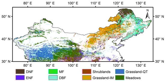
Figure 1.
Eight biomes of temperate China, including deciduous needleleaf forests (DNF), evergreen needleleaf forests (ENF), mixed forests (MF), deciduous broadleaf forests (DBF), shrublands, grasslands in Inner Mongolia (GRA-IM), grasslands in Qinghai-Tibet Plateau (GRA-QT), and meadows.
2.2. GIMMS NDVI3g Dataset
The GIMMS NDVI 3rd generation (NDVI3g) datasets with a 1/12° × 1/12° spatial resolution and 15-day intervals were used in this study, derived from NOAA AVHRR sensor for the period 2000–2015. These data can be obtained from here (https://ecocast.arc.nasa.gov/data/pub/gimms/, accessed on 13 January 2022). The GIMMS NDVI3g datasets have been corrected to minimize the effects of aerosol, clouds, solar angle, sensor errors and degradation and can be applicable for evaluate the long-term trends in vegetation activities [12,37,41,42]. In order to reduce the effects of clouds, spectral characteristics and residual atmospheric effects, the maximum value composites method was adopted for the NDVI products [43]. In addition, NDVI quality flags are implanted in the data files, which provide references about per-pixel NDVI status. Flag values of the NDVI3g data (NDVI3g.v1) range from 0 to 2, NDVI (flag = 1) are acquired from spline interpolation, whereas flag = 0 indicates good value and flag = 2 indicates possible snow or cloud cover. NDVI data with flag values of 0 and 1 were used in this research.
2.3. MODIS NDVI Dataset
The latest version (Collection 6) Terra MODIS NDVI product with 1 × 1 km2 spatial resolution and 16-day temporal intervals (MOD13A2) were used in this study. The MOD13A2 data product was obtained from Land Processes Distributed Active Archive Center (LP DAAC) data pool (https://ladsweb.modaps.eosdis.nasa.gov/, accessed on 15 January 2022). The MOD13A2 products are obtained from atmospherically corrected surface reflectance using the constrained view angle maximum value composite method, which is used to address the angular variations that are inherent to most space-based imaging instruments and reduce the impacts of clouds and aerosols [15]. All images from 2000 to 2015 were utilized to be consistent with the temporal extent of GIMMS NDVI3g datasets (because there is no data about MOD13A2 in the first two months of the year 2000, mean values for the first two months of 2001–2015 were calculated to obtain a full year of data). Similar to the GIMMS NDVI3g dataset, the MOD13A2 datasets contain a data quality assessment (QA) including references on overall usefulness and cloud on per-pixel status. We excluded pixels with quality flags that are clouds and atmospheric aerosol using the methodology according to [17,44]. Additionally, it was noteworthy that the expression of NDVI is non-linear transformation and the spatial resampling of MOD13A2 1 km data should not performed directly on the NDVI but rather on the surface reflectance. Therefore, the corresponding MOD13A2 1 km red and near-infrared bands were resampled to match the spatial resolution of GIMMS NDVI data using the nearest neighbor algorithm before calculating NDVI.
2.4. Reconstruction of NDVI Temporal Trajectory and Detection of Phenological Metrics
The GIMMS NDVI3g and MODIS NDVI long-term datasets were analyzed using the time-series analysis program TIMESAT version 3.2 [45]. We used the Asymmetric Gaussian model (AG), Double Logistic method (DL), and Savitzky-Golay filter (SG) to establish a smooth NDVI time series curve. Based on the reconstructed NDVI time series, the main phenological metrics SOS and EOS were identified as points in time where the value has increased or decreased by a threshold. A 30% threshold for both SOS and EOS was selected as the optimal value according to analyzing the fitted time-series curves. Details about our methods can be found in the corresponding papers [45,46,47].
2.5. Data Analysis
We applied the least squares linear regression from 2000 to 2015 to access the temporal trends of the two growing season (March–November) NDVI datasets throughout the whole of temperate China. Then, the Pearson’s correlation analysis was used to examine the uniformity for the two datasets pixel by pixel based on the multi-year (2000–2015) averaged NDVI. To quantify the discrepancy between GIMMS and MODIS data NDVI and extracted phenology, we made the difference among the corresponding data metrics. Considering the phenology metrics may not meet the assumptions for parametric analysis, the study used the Theil-Sen trend analysis and nonparametric Mann-Kendall test to compare the consistencies of SOS and EOS between GIMMS and MODIS datasets [48].
For time-series data, the Sen’s slope was calculated between two random points, and then the median value was chosen as the final slope in Equation (1).
where xi and xj are data values at times ti and tj (i > j), respectively. When β > 0, it means the time series shows an upward trend, otherwise, it shows a downward trend.
To test the significance of the time series, the Mann-Kendall statistic S were firstly constructed in Equations (2) and (3). For n ≥ 10, the statistic S approximately normally distributed with the mean and variance in Equation (4). Then the standardized Z test statistic was computed by Equation (5).
where n is the number of data points, g is the number of tied groups and tp denotes the number of ties of extent p. By comparing the Z value with the standard normal variance at the pre-specified level of statistical significance, we could access the significance of trend. The phenology parameters were related to a significant trend when the significance level was set 95% in this study. All statistical analyses and models were carried out in R (version 4.2.0) with “trend” package.
3. Results
3.1. Comparison between GIMMS NDVI3g and MODIS NDVI
Figure 2 showed the annual changes of the spatially mean NDVI values in temperate China during 2000–2015. The spatially mean GIMMS NDVI was significantly higher than MODIS NDVI for temperate China (Figure 2a). During the study period, both of them displayed significant increasing trends (p < 0.05). A pixel-by-pixel correlation analysis was conducted on the annual GIMMS and MODIS NDVI over temperate China from 2000 to 2015. For the whole study area, the GIMMS versus MODIS NDVI relationship had an R2 of 0.9209 and they were generally on a 1:1 relationship line (Figure 2b). Spatially, the multi-year mean GIMMS NDVI was higher than MODIS NDVI in 77.5% of temperate China with approximately 55.5% of the total pixels have values between 0 and 0.05 (Figure 3).
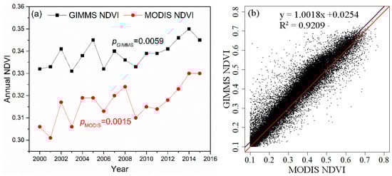
Figure 2.
(a) Annual changes of the spatially mean NDVI based on the GIMMS and MODIS datasets during 2000–2015; (b) The scatter plot of the multi-year averaged NDVI for the two datasets from 2000–2015.
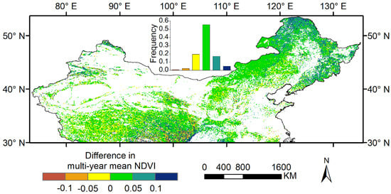
Figure 3.
Discrepancy in the multi-year mean NDVI between GIMMS and MODIS datasets during 2000–2015.
Figure 4 showed the mean annual NDVI in overall (entire study area) and eight biomes from these two NDVI datasets. For different biomes, GIMMS and MODIS NDVI were moderately well correlated. In spite of the general agreement, some persistent differences remained. The agreement between GIMMS NDVI and MODIS NDVI for all biomes in senescence phase were better than that in green-up phase. Particularly, the differences between these two NDVI datasets for forests (including DNF, ENF, MF and DBF) in green-up phase were obvious smaller than that for shrublands, grasslands-IM, grasslands-QT and meadows.
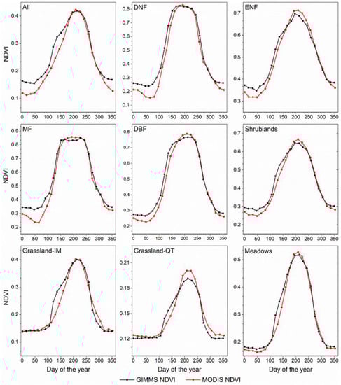
Figure 4.
Mean annual NDVI from 2000 to 2015 between GIMMS and MODIS datasets for different biomes.
3.2. Spatial Differences in Multi-Year Mean Phenology
The spatial distributions of absolute differences of SOS and EOS over temperate China between GIMMS and MODIS data for different methods were summarized from 2000 to 2015 (Figure 5). For each method, the results of the discrepancies between the multi-year mean SOSg (SOS derived from GIMMS NDVI) and SOSm (SOS derived from MODIS NDVI) by the three methods are overall very similar, whereas large discrepancies were found for multi-year mean SOSg and SOSm. The inconsistencies were generally less than 30 days in SOS across the study area (89.89% for AG, 89.28% for DL and 91.98% for SG). In particular, the pixels about the discrepancies of less than 10 days between SOSg and SOSm accounted for 44.51%, 43.78% and 48.74% of the total pixels for AG, DL and SG methods, respectively. At spatial scale, there were no apparent changes of the differences between SOSg and SOSm with methods, and then the pixels about the discrepancies of less than 20 days between SOSg and SOSm were mostly distributed in the central and northeastern China.
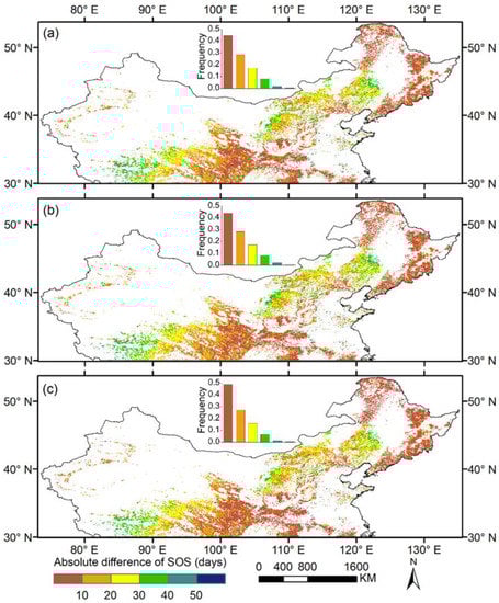
Figure 5.
Discrepancies of the multi-year mean SOS between GIMMS and MODIS datasets during 2000–2015 for different methods: (a) Asymmetric Gaussians (AG); (b) Double Logistic functions (DL); (c) Savitzky-Golay filter (SG).
Compared to SOS, for the three methods, the inconsistencies between the multi-year mean EOSg (EOS derived from GIMMS NDVI) and EOSm (EOS derived from MODIS NDVI) were relatively small (Figure 6). With regards to the pixels about discrepancies of less than 20 days in EOS, the proportions were 96.19%, 96.61% and 96.75% for AG, DL and SG, respectively. In addition, the pixels about discrepancies of less than 10 days in EOS were significantly more than that in SOS (72.29% for AG, 73.51% for DL and 70.14% for SG in EOS). Spatially, the pixels about the discrepancies of less than 20 days between EOSg and EOSm were distributed in most areas of temperate China.
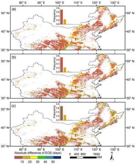
Figure 6.
Discrepancies of the multi-year mean EOS between GIMMS and MODIS datasets during 2000–2015 for different methods: (a) Asymmetric Gaussians (AG); (b) Double Logistic functions (DL); (c) Savitzky-Golay filter (SG).
3.3. SOS and EOS Differences across Eight Biomes
The SOS and EOS differences were calculated for the GIMMS and MODIS datasets from 2000 to 2015 in eight biomes for different methods. For each method, the differences of SOS in forests (DNF, ENF, MF and DBF) were clearly less than that in shrublands, grasslands-IM, grasslands-QT and meadows (Figure 7). Further analysis showed that for most biomes of forests except ENF, the pixels about the discrepancies of less than 10 days between SOSg and SOSm accounted for more than 65% of the total pixels. Nevertheless, the proportions for the pixels about the discrepancies of less than 10 days between SOSg and SOSm in grasslands-IM, grasslands-QT were unexpectedly lower than 20% of the total pixels.
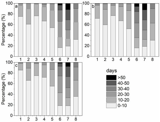
Figure 7.
Allocation of SOS discrepancy between GIMMS and MODIS datasets at 0–10, 10–20, 20–30, 30–40, 40–50, and more than 50 days, across eight biomes for different methods: (a) AG; (b) DL; (c) SG. (Number 1–8 represents DNF, ENF, MF, DBF, shrublands, grasslands-IM, grasslands-QT and meadows, respectively).
As shown in Figure 8, there was somewhat dissimilarity in the overall results of the differences between EOSg and EOSm compared to the results of SOS. For each method, the differences of EOS in forests (DNF, ENF, MF and DBF) were relatively greater than that in SOS (the proportions for the pixels about the discrepancies of less than 10 days between EOSg and EOSm were mostly lower than 65% of the total pixels). However, the pixels about the discrepancies of less than 10 days between EOSg and EOSm in shrublands, grasslands-IM, grasslands-QT and meadows occupied mostly more than 60% of the total pixels (more than 80% especially in grasslands-QT and meadows), which means that the differences of EOS in shrublands, grasslands-IM, grasslands-QT and meadows were obviously lower than that in SOS.
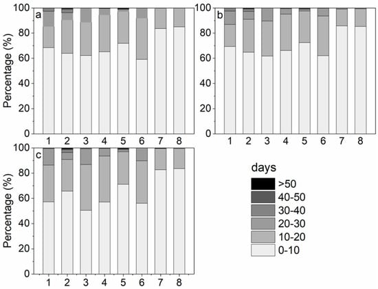
Figure 8.
Allocation of EOS discrepancy between GIMMS and MODIS datasets at 0–10, 10–20, 20–30, 30–40, 40–50, and more than 50 days, across eight biomes for different methods: (a) AG; (b) DL; (c) SG. (Number 1–8 represents DNF, ENF, MF, DBF, shrublands, grasslands-IM, grasslands-QT and meadows, respectively).
3.4. Comparison of Phenology Trends between GIMMS and MODIS Datasets
Generally, trend analysis was conducted with 16 years of SOS or EOS trends between GIMMS and MODIS datasets about different methods (Table 1). For both datasets, SOS and EOS trends for 16 years were shown insignificant in most areas of temperate China. For SOS trends, the pixels accounted for shared significantly advanced trends from the two datasets were more than that shared significantly delayed trends. However, the EOS trends between GIMMS and MODIS datasets were opposite to that in SOS. Moreover, the proportion of pixels about significantly opposite trends was low. In addition, for each method, the proportion of pixels that significantly SOS trend only for one dataset (22.79% for AG, 19.72% for DL, and 18.33% for SG) were higher than that in EOS trend (17.77% for AG, 18.65% for DL, and 15.84% for SG).

Table 1.
Summary statistics for comparison of SOS or EOS trends between GIMMS and MODIS datasets about different methods (p < 0.05).
Table 2 shows the SOS or EOS trends from 2000 to 2015 across eight biomes for different methods. Only for grasslands-QT and meadows, SOSg had a significantly delayed trend for all three methods. SOSm of ENF, shrublands and grasslands-IM had significantly advanced trends for all three methods, and SOSm of DBF also had a significantly advanced trend for AG and DL methods. For all biomes, EOSg had no significant trend for all three methods. The EOSm of MF had a significantly delayed trend for all three methods, and the EOSm of DBF also had a significantly delayed trend for AG and DL methods.
Table 2.
Comparison of SOS or EOS trends between GIMMS and MODIS datasets across eight biomes for different methods (p < 0.05).
4. Discussion
Based on GIMMS and MODIS data in temperate China from 2000 to 2015, this study compared time series NDVI and key phenological metrics (SOS and EOS). The comparison revealed that there were large discrepancies between the two datasets. Previous analysis indicated similar consequences for phenological metrics between GIMMS and MODIS in Europe [23] and Northern Hemisphere [26]. Overall, it was found in temperate China that about 45% of pixels had SOS differences less than 10 days (EOS difference was smaller, which the proportion was about 70%). As for the different biomes in green-up phase, the differences of SOS in forests (including DNF, ENF, MF and DBF) were obviously less than that in shrublands, grasslands-IM, grasslands-QT and meadows (Figure 7), because the agreement between NDVI from two satellite datasets for forests in green-up phase were better than that for shrublands, grasslands-IM, grasslands-QT and meadows (Figure 4). A similar perspective has emerged from the results of EOS for different biomes in senescence phase. This may be ascribed to the effect of the differences between NDVI from two satellite datasets. Specifically, the AVHRR and MODIS have different instrumental characteristics, especially the wavelengths with the red and near-infrared bands required to obtain NDVI are different. The red and near-infrared bands for AVHRR sensors are 585–680 nm and 730–980 nm, respectively, and these bands were significantly influenced by the absorption of water vapor in the atmosphere. The bandwidths about MODIS are narrower than that about AVHRR, with the red (620–670 nm) and near-infrared (841–876 nm) bands. MODIS removes the influence of the water vapor band in the near-infrared band, while the red band is more sensitive to the absorption of chlorophyll [49]. The differences in the spectral characteristics of these bands (such as the central value of the band, the width of the band, etc.) between AVHRR and MODIS may cause the discrepancies in the process of extracting phenology from NDVI time series at the green-up or senescence phase. Figure 9 further showed the difference trend of mean NDVI between GIMMS and MODIS in spring and autumn. Overall, the difference in spring was higher than that of in autumn, which to some extent also explained the larger and smaller discrepancy in SOS and EOS, respectively.
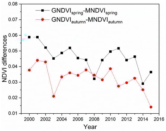
Figure 9.
The mean NDVI difference between GIMMS and MODIS during spring (March–May) and autumn (September–November).
The influences of discrepancies between different NDVI datasets on phenology monitoring indicate there is a caution when analyzing long-term phenological trends. Recent studies represented that the NDVI datasets from GIMMS and MODIS were applied to detect changes in vegetation phenology at large spatio-temporal scales [20,21,50,51,52]. More especially, Zhang et al. [26] showed that the GIMMS NDVI3g and MODIS NDVI reflected varying degrees of phenological trends in the Northern Hemisphere, including the opposite trends. Similar findings (Table 1 and Table 2) were also found in our study, with large differences of phenological trends between GIMMS and MODIS datasets in temperate China from 2000 to 2015. Both the two datasets exhibited significantly trends (including advancing and delayed trends) with small proportion of pixels. Additionally, there are basically no similar significantly trends of phenology across all the biomes, which to a large extent also indicates the discrepancy between the two datasets.
We used three phenology extraction methods for extracting phenological parameters to avoid bias from a single approach, which is also a common practice used in other studies [53,54]. The extraction methods can affect the results of time-series inversion about phenology, according to several studies [55,56,57]. For instance, Cong et al. [36] compared five common methods in extracting spring phenology with NDVI datasets derived from SPOT satellites in temperate China. The findings indicated that there was a similar spatial pattern of spring phenology estimated by five different methods, but the phenological dates were significantly varying. Moreover, our results also suggest that the overall patterns of phenological trends from these three methods were relatively conformable, but different methods may also lead to uncertainties in the magnitude of phenological trends. In addition, in our study, in general, these methods yield relatively small differences in phenology, and there is no need to substitute one method for all others.
This study highlighted the similarity and discrepancies of vegetation phenology between GIMMS and MODIS datasets rather than deciding whether GIMMS or MODIS dataset was more advantageous to extract phenological information. We found that the inconsistencies of phenological parameters between these two datasets were in some degree attributed to sensor differences based on same data preprocessing and phenology extraction methods. Moreover, it was important to notice that classification criteria of biomes might impact the values of phenological parameters in different biomes. In this study, a 1:1,000,000 vegetation data of China in 2001 from EBVMC was used to determine the classification of different biomes. In fact, however, the ranges of different biomes might vary with year during 2000–2015, and it could influence the results and data analysis of phenology in different biomes when studying long-term time series satellite-derived datasets. In addition, the values of phenology derived from satellite sensors are also affected by the quality of data [21], and spatio-temporal resolutions [58] of time series datasets.
5. Conclusions
This study comprehensively performed a comparative analysis of the phenological characteristics of different biomes in temperate China during 2000–2015 based on NDVI datasets from GIMMS and MODIS. Spatio-temporal patterns of NDVI, SOS or EOS, and their trends between these two datasets in the entire region and eight biomes were analyzed. The primary findings are summarized as follows:
- (1)
- The discrepancies of instrumental characteristics between GIMMS and MODIS sensors induced the inconsistencies of NDVI. Overall, the spatially averaged GIMMS NDVI across the study area was significantly higher than MODIS NDVI. For different biomes, the consistencies between GIMMS NDVI and MODIS NDVI for all biomes in senescence phase were better than that in green-up phase. Furthermore, the differences between these two NDVI datasets for forests in green-up phases were obviously smaller than those for shrublands, grasslands-IM, grasslands-QT and meadows.
- (2)
- The differences in NDVI between GIMMS and MODIS induced the inconsistencies between phenology derived from the two datasets. The discrepancies between the multi-year mean SOSg and SOSm were large for three methods of extracting phenology. However, the inconsistencies between the multi-year mean EOSg and EOSm were relatively small compared to SOS. For biomes, the differences of SOS in forests were clearly less than that in shrublands, grasslands-IM, grasslands-QT and meadows. For EOS, however, the differences of EOS in forests were relatively greater than that in SOS. Moreover, the differences of EOS in shrublands, grasslands-IM, grasslands-QT and meadows were obviously lower than that in SOS.
- (3)
- SOS and EOS trends (including advanced, delayed and opposite trends) during 2000–2015 for three methods were insignificant in most areas of temperate China. For most biomes, phenological trends were also insignificant. In addition, a large discrepancy of SOS and EOS trends between GIMMS and MODIS datasets appeared in different biomes.
- (4)
- The discrepancies of phenological parameters and their trends over the entire region and different biomes highlighted that in order to reduce the uncertainty in estimating the land surface phenology and further analyze the trend, it is necessary to combine the result for several sensors, such as by inter-calibrating the time series across multiple-sensor datasets, especially for some specific biomes (e.g., grasslands in temperate China).
Future studies should put more emphasis on the demand for the phenology derived from these sensors compared and validated with field phenology observation, eddy covariance measurements, solar-induced chlorophyll fluorescence retrieved from GOSAT or GOME sensors, and VI products derived from other remote sensors (e.g., MERIS MTCI, SPOT, and Landsat). Furthermore, follow-up research should focus on comparing the variations in land surface phenology in temperate China between GIMMS and MODIS NDVI datasets for their response to climate change.
Author Contributions
All authors offered assistance for this study and manuscript preparation. J.X., K.H. and J.Z. developed the original idea and wrote the paper; J.X., Y.L. and J.Z. conducted data analysis; J.X., K.H., P.R. and J.Z. revised the paper. All authors have read and agreed to the published version of the manuscript.
Funding
This research was funded by the National Key Research & Development Program of China (2018YFA0606101), the National Natural Science Foundation of China (41801185), the Strategic Priority Research Program (category A) of Chinese Academy of Sciences (XDA20020302).
Data Availability Statement
All data can be accessed through the provided website.
Acknowledgments
We would like to thank to the editors and reviewers, who have put great effort into their comments on this manuscript. We would also thank the data publishers and funding agencies.
Conflicts of Interest
The authors declare that they have no conflict of interest.
References
- Piao, S.; Friedlingstein, P.; Ciais, P.; Viovy, N.; Demarty, J. Growing season extension and its impact on terrestrial carbon cycle in the Northern Hemisphere over the past 2 decades. Glob. Biogeochem. Cycles 2007, 21, GB3018. [Google Scholar] [CrossRef]
- Churkina, G.; Schimel, D.; Braswell, B.H.; Xiao, X. Spatial analysis of growing season length control over net ecosystem exchange. Glob. Chang. Biol. 2005, 11, 1777–1787. [Google Scholar] [CrossRef]
- Barichivich, J.; Briffa, K.R.; Myneni, R.B.; Osborn, T.J.; Melvin, T.M.; Ciais, P.; Piao, S.; Tucker, C. Large-scale variations in the vegetation growing season and annual cycle of atmospheric CO2 at high northern latitudes from 1950 to 2011. Glob. Chang. Biol. 2013, 19, 3167–3183. [Google Scholar] [CrossRef]
- Peñuelas, J.; Rutishauser, T.; Filella, I. Phenology Feedbacks on Climate Change. Science 2009, 324, 887–888. [Google Scholar] [CrossRef] [PubMed]
- Piao, S.; Liu, Z.; Wang, T.; Peng, S.; Ciais, P.; Huang, M.; Ahlstrom, A.; Burkhart, J.F.; Chevallier, F.; Janssens, I.A.; et al. Weakening temperature control on the interannual variations of spring carbon uptake across northern lands. Nat. Clim. Chang. 2017, 7, 359. [Google Scholar] [CrossRef]
- Vrieling, A.; Meroni, M.; Darvishzadeh, R.; Skidmore, A.K.; Wang, T.; Zurita-Milla, R.; Oosterbeek, K.; O’Connor, B.; Paganini, M. Vegetation phenology from Sentinel-2 and field cameras for a Dutch barrier island. Remote Sens. Environ. 2018, 215, 517–529. [Google Scholar] [CrossRef]
- Myneni, R.B.; Keeling, C.D.; Tucker, C.J.; Asrar, G.; Nemani, R.R. Increased plant growth in the northern high latitudes from 1981 to 1991. Nature 1997, 386, 698. [Google Scholar] [CrossRef]
- Piao, S.; Fang, J.; Zhou, L.; Ciais, P.; Zhu, B. Variations in satellite-derived phenology in China’s temperate vegetation. Glob. Chang. Biol. 2006, 12, 672–685. [Google Scholar] [CrossRef]
- Heumann, B.W.; Seaquist, J.W.; Eklundh, L.; Jönsson, P. AVHRR derived phenological change in the Sahel and Soudan, Africa, 1982–2005. Remote Sens. Environ. 2007, 108, 385–392. [Google Scholar] [CrossRef]
- Zhu, W.; Tian, H.; Xu, X.; Pan, Y.; Chen, G.; Lin, W. Extension of the growing season due to delayed autumn over mid and high latitudes in North America during 1982–2006. Glob. Ecol. Biogeogr. 2012, 21, 260–271. [Google Scholar] [CrossRef]
- Zhao, J.; Zhang, H.; Zhang, Z.; Guo, X.; Li, X.; Chen, C. Spatial and Temporal Changes in Vegetation Phenology at Middle and High Latitudes of the Northern Hemisphere over the Past Three Decades. Remote Sens. 2015, 7, 10973–10995. [Google Scholar] [CrossRef]
- Pinzon, J.; Tucker, C. A Non-Stationary 1981–2012 AVHRR NDVI3g Time Series. Remote Sens. 2014, 6, 6929–6960. [Google Scholar] [CrossRef]
- Jiang, N.; Zhu, W.; Zheng, Z.; Chen, G.; Fan, D. A Comparative Analysis between GIMSS NDVIg and NDVI3g for Monitoring Vegetation Activity Change in the Northern Hemisphere during 1982–2008. Remote Sens. 2013, 5, 4031–4044. [Google Scholar] [CrossRef]
- Zhu, Z.; Bi, J.; Pan, Y.; Ganguly, S.; Anav, A.; Xu, L.; Samanta, A.; Piao, S.; Nemani, R.; Myneni, R. Global Data Sets of Vegetation Leaf Area Index (LAI)3g and Fraction of Photosynthetically Active Radiation (FPAR)3g Derived from Global Inventory Modeling and Mapping Studies (GIMMS) Normalized Difference Vegetation Index (NDVI3g) for the Period 1981 to 2011. Remote Sens. 2013, 5, 927–948. [Google Scholar] [CrossRef]
- Huete, A.; Didan, K.; Miura, T.; Rodriguez, E.P.; Gao, X.; Ferreira, L.G. Overview of the radiometric and biophysical performance of the MODIS vegetation indices. Remote Sens. Environ. 2002, 83, 195–213. [Google Scholar] [CrossRef]
- Fensholt, R.; Rasmussen, K.; Nielsen, T.T.; Mbow, C. Evaluation of earth observation based long term vegetation trends—Intercomparing NDVI time series trend analysis consistency of Sahel from AVHRR GIMMS, Terra MODIS and SPOT VGT data. Remote Sens. Environ. 2009, 113, 1886–1898. [Google Scholar] [CrossRef]
- Fensholt, R.; Proud, S.R. Evaluation of Earth Observation based global long term vegetation trends—Comparing GIMMS and MODIS global NDVI time series. Remote Sens. Environ. 2012, 119, 131–147. [Google Scholar] [CrossRef]
- Justice, C.O.; Townshend, J.R.G.; Vermote, E.F.; Masuoka, E.; Wolfe, R.E.; Saleous, N.; Roy, D.P.; Morisette, J.T. An overview of MODIS Land data processing and product status. Remote Sens. Environ. 2002, 83, 3–15. [Google Scholar] [CrossRef]
- Wu, W.; Sun, Y.; Xiao, K.; Xin, Q. Development of a global annual land surface phenology dataset for 1982–2018 from the AVHRR data by implementing multiple phenology retrieving methods. Int. J. Appl. Earth Obs. Geoinf. 2021, 103, 102487. [Google Scholar] [CrossRef]
- Garonna, I.; de Jong, R.; Schaepman, M.E. Variability and evolution of global land surface phenology over the past three decades (1982–2012). Glob. Chang. Biol. 2016, 22, 1456–1468. [Google Scholar] [CrossRef]
- Zhang, X.; Liu, L.; Yan, D. Comparisons of global land surface seasonality and phenology derived from AVHRR, MODIS, and VIIRS data. J. Geophys. Res. Biogeosci. 2017, 122, 1506–1525. [Google Scholar] [CrossRef]
- Moon, M.; Zhang, X.; Henebry, G.M.; Liu, L.; Gray, J.M.; Melaas, E.K.; Friedl, M.A. Long-term continuity in land surface phenology measurements: A comparative assessment of the MODIS land cover dynamics and VIIRS land surface phenology products. Remote Sens. Environ. 2019, 226, 74–92. [Google Scholar] [CrossRef]
- Atzberger, C.; Klisch, A.; Mattiuzzi, M.; Vuolo, F. Phenological Metrics Derived over the European Continent from NDVI3g Data and MODIS Time Series. Remote Sens. 2014, 6, 257–284. [Google Scholar] [CrossRef]
- Brown, M.E.; Pinzon, J.E.; Didan, K.; Morisette, J.T.; Tucker, C.J. Evaluation of the consistency of long-term NDVI time series derived from AVHRR, SPOT-vegetation, SeaWiFS, MODIS, and Landsat ETM+ sensors. IEEE Trans. Geosci. Remote Sens. 2006, 44, 1787–1793. [Google Scholar] [CrossRef]
- Gallo, K.; Ji, L.; Reed, B.; Eidenshink, J.; Dwyer, J. Multi-platform comparisons of MODIS and AVHRR normalized difference vegetation index data. Remote Sens. Environ. 2005, 99, 221–231. [Google Scholar] [CrossRef]
- Zhang, J.; Zhao, J.; Wang, Y.; Zhang, H.; Zhang, Z.; Guo, X. Comparison of land surface phenology in the Northern Hemisphere based on AVHRR GIMMS3g and MODIS datasets. ISPRS J. Photogramm. Remote Sens. 2020, 169, 1–16. [Google Scholar] [CrossRef]
- Heqing, Z.; Gensuo, J.; Howard, E. Recent changes in phenology over the northern high latitudes detected from multi-satellite data. Environ. Res. Lett. 2011, 6, 045508. [Google Scholar] [CrossRef]
- Kern, A.; Marjanović, H.; Barcza, Z. Evaluation of the Quality of NDVI3g Dataset against Collection 6 MODIS NDVI in Central Europe between 2000 and 2013. Remote Sens. 2016, 8, 955. [Google Scholar] [CrossRef]
- Zhang, G.; Zhang, Y.; Dong, J.; Xiao, X. Green-up dates in the Tibetan Plateau have continuously advanced from 1982 to 2011. Proc. Natl. Acad. Sci. USA 2013, 110, 4309–4314. [Google Scholar] [CrossRef]
- Zhou, L.; Tucker, C.J.; Kaufmann, R.K.; Slayback, D.; Shabanov, N.V.; Myneni, R.B. Variations in northern vegetation activity inferred from satellite data of vegetation index during 1981 to 1999. J. Geophys. Res. Atmos. 2001, 106, 20069–20083. [Google Scholar] [CrossRef]
- Liu, Q.; Fu, Y.H.; Zhu, Z.; Liu, Y.; Liu, Z.; Huang, M.; Janssens, I.A.; Piao, S. Delayed autumn phenology in the Northern Hemisphere is related to change in both climate and spring phenology. Glob. Chang. Biol. 2016, 22, 3702–3711. [Google Scholar] [CrossRef] [PubMed]
- Ge, Q.; Wang, H.; Rutishauser, T.; Dai, J. Phenological response to climate change in China: A meta-analysis. Glob. Chang. Biol. 2015, 21, 265–274. [Google Scholar] [CrossRef] [PubMed]
- Shushi, P.; Anping, C.; Liang, X.; Chunxiang, C.; Jingyun, F.; Ranga, B.M.; Jorge, E.P.; Compton, J.T.; Shilong, P. Recent change of vegetation growth trend in China. Environ. Res. Lett. 2011, 6, 044027. [Google Scholar] [CrossRef]
- Chen, X.; Hu, B.; Yu, R. Spatial and temporal variation of phenological growing season and climate change impacts in temperate eastern China. Glob. Chang. Biol. 2005, 11, 1118–1130. [Google Scholar] [CrossRef]
- Wu, X.; Liu, H. Consistent shifts in spring vegetation green-up date across temperate biomes in China, 1982–2006. Glob. Chang. Biol. 2013, 19, 870–880. [Google Scholar] [CrossRef]
- Cong, N.; Piao, S.; Chen, A.; Wang, X.; Lin, X.; Chen, S.; Han, S.; Zhou, G.; Zhang, X. Spring vegetation green-up date in China inferred from SPOT NDVI data: A multiple model analysis. Agric. For. Meteorol. 2012, 165, 104–113. [Google Scholar] [CrossRef]
- Liu, Q.; Fu, Y.H.; Zeng, Z.; Huang, M.; Li, X.; Piao, S. Temperature, precipitation, and insolation effects on autumn vegetation phenology in temperate China. Glob. Chang. Biol. 2016, 22, 644–655. [Google Scholar] [CrossRef]
- Slayback, D.A.; Pinzon, J.E.; Los, S.O.; Tucker, C.J. Northern hemisphere photosynthetic trends 1982–99. Glob. Chang. Biol. 2003, 9, 1–15. [Google Scholar] [CrossRef]
- White, M.A.; Thornton, P.E.; Running, S.W. A continental phenology model for monitoring vegetation responses to interannual climatic variability. Glob. Biogeochem. Cycles 1997, 11, 217–234. [Google Scholar] [CrossRef]
- Jeong, S.-J.; Ho, C.-H.; Gim, H.-J.; Brown, M.E. Phenology shifts at start vs. end of growing season in temperate vegetation over the Northern Hemisphere for the period 1982–2008. Glob. Chang. Biol. 2011, 17, 2385–2399. [Google Scholar] [CrossRef]
- Piao, S.; Cui, M.; Chen, A.; Wang, X.; Ciais, P.; Liu, J.; Tang, Y. Altitude and temperature dependence of change in the spring vegetation green-up date from 1982 to 2006 in the Qinghai-Xizang Plateau. Agric. For. Meteorol. 2011, 151, 1599–1608. [Google Scholar] [CrossRef]
- Cong, N.; Wang, T.; Nan, H.; Ma, Y.; Wang, X.; Myneni, R.B.; Piao, S. Changes in satellite-derived spring vegetation green-up date and its linkage to climate in China from 1982 to 2010: A multimethod analysis. Glob. Chang. Biol. 2013, 19, 881–891. [Google Scholar] [CrossRef] [PubMed]
- Tucker, C.J.; Pinzon, J.E.; Brown, M.E.; Slayback, D.A.; Pak, E.W.; Mahoney, R.; Vermote, E.F.; El Saleous, N. An extended AVHRR 8-km NDVI dataset compatible with MODIS and SPOT vegetation NDVI data. Int. J. Remote Sens. 2005, 26, 4485–4498. [Google Scholar] [CrossRef]
- Samanta, A.; Ganguly, S.; Hashimoto, H.; Devadiga, S.; Vermote, E.; Knyazikhin, Y.; Nemani, R.R.; Myneni, R.B. Amazon forests did not green-up during the 2005 drought. Geophys. Res. Lett. 2010, 37, L05401. [Google Scholar] [CrossRef]
- Jönsson, P.; Eklundh, L. TIMESAT—A program for analyzing time-series of satellite sensor data. Comput. Geosci. 2004, 30, 833–845. [Google Scholar] [CrossRef]
- Stanimirova, R.; Cai, Z.; Melaas, E.K.; Gray, J.M.; Eklundh, L.; Jönsson, P.; Friedl, M.A. An empirical assessment of the MODIS land cover dynamics and TIMESAT land surface phenology algorithms. Remote Sens. 2019, 11, 2201. [Google Scholar] [CrossRef]
- Zu, J.; Zhang, Y.; Huang, K.; Liu, Y.; Chen, N.; Cong, N. Biological and climate factors co-regulated spatial-temporal dynamics of vegetation autumn phenology on the Tibetan Plateau. Int. J. Appl. Earth Obs. Geoinf. 2018, 69, 198–205. [Google Scholar] [CrossRef]
- Guo, M.; Li, J.; He, H.; Xu, J.; Jin, Y. Detecting Global Vegetation Changes Using Mann-Kendal (MK) Trend Test for 1982–2015 Time Period. Chin. Geogr. Sci. 2018, 28, 907–919. [Google Scholar] [CrossRef]
- Miura, T.; Turner, J.P.; Huete, A.R. Spectral compatibility of the NDVI across VIIRS, MODIS, and AVHRR: An analysis of atmospheric effects using EO-1 Hyperion. IEEE Trans. Geosci. Remote Sens. 2012, 51, 1349–1359. [Google Scholar] [CrossRef]
- Buitenwerf, R.; Rose, L.; Higgins, S.I. Three decades of multi-dimensional change in global leaf phenology. Nat. Clim. Chang. 2015, 5, 364–368. [Google Scholar] [CrossRef]
- Wang, X.; Piao, S.; Xu, X.; Ciais, P.; MacBean, N.; Myneni, R.B.; Li, L. Has the advancing onset of spring vegetation green-up slowed down or changed abruptly over the last three decades? Glob. Ecol. Biogeogr. 2015, 24, 621–631. [Google Scholar] [CrossRef]
- Hmimina, G.; Dufrêne, E.; Pontailler, J.-Y.; Delpierre, N.; Aubinet, M.; Caquet, B.; De Grandcourt, A.; Burban, B.; Flechard, C.; Granier, A. Evaluation of the potential of MODIS satellite data to predict vegetation phenology in different biomes: An investigation using ground-based NDVI measurements. Remote Sens. Environ. 2013, 132, 145–158. [Google Scholar] [CrossRef]
- Cai, Z.; Jönsson, P.; Jin, H.; Eklundh, L. Performance of smoothing methods for reconstructing NDVI time-series and estimating vegetation phenology from MODIS data. Remote Sens. 2017, 9, 1271. [Google Scholar] [CrossRef]
- Li, N.; Zhan, P.; Pan, Y.; Zhu, X.; Li, M.; Zhang, D. Comparison of remote sensing time-series smoothing methods for grassland spring phenology extraction on the Qinghai–Tibetan Plateau. Remote Sens. 2020, 12, 3383. [Google Scholar] [CrossRef]
- Ding, M.; Li, L.; Zhang, Y.; Sun, X.; Liu, L.; Gao, J.; Wang, Z.; Li, Y. Start of vegetation growing season on the Tibetan Plateau inferred from multiple methods based on GIMMS and SPOT NDVI data. J. Geogr. Sci. 2015, 25, 131–148. [Google Scholar] [CrossRef]
- Zheng, Z.; Zhu, W. Uncertainty of remote sensing data in monitoring vegetation phenology: A comparison of MODIS C5 and C6 vegetation index products on the Tibetan Plateau. Remote Sens. 2017, 9, 1288. [Google Scholar] [CrossRef]
- White, M.A.; de Beurs, K.M.; Didan, K.; Inouye, D.W.; Richardson, A.D.; Jensen, O.P.; O’keefe, J.; Zhang, G.; Nemani, R.R.; van Leeuwen, W.J. Intercomparison, interpretation, and assessment of spring phenology in North America estimated from remote sensing for 1982–2006. Glob. Chang. Biol. 2009, 15, 2335–2359. [Google Scholar] [CrossRef]
- Peng, D.; Zhang, X.; Zhang, B.; Liu, L.; Liu, X.; Huete, A.R.; Huang, W.; Wang, S.; Luo, S.; Zhang, X.; et al. Scaling effects on spring phenology detections from MODIS data at multiple spatial resolutions over the contiguous United States. ISPRS J. Photogramm. Remote Sens. 2017, 132, 185–198. [Google Scholar] [CrossRef]
Publisher’s Note: MDPI stays neutral with regard to jurisdictional claims in published maps and institutional affiliations. |
© 2022 by the authors. Licensee MDPI, Basel, Switzerland. This article is an open access article distributed under the terms and conditions of the Creative Commons Attribution (CC BY) license (https://creativecommons.org/licenses/by/4.0/).