Investigating the Impact of the Spatiotemporal Bias Correction of Precipitation in CMIP6 Climate Models on Drought Assessments

Abstract

Precipitation of future climate models is critical for the assessments of future drought but contains large systematic biases over the Tibetan Plateau. Although the common precipitation bias correction method, quantile mapping has achieved remarkable results in terms of temporal bias correction, it does not consider the spatial distribution of bias. Furthermore, the extent to which precipitation bias affects drought estimation remains unclear. In our study, we take the Qinghai–Tibet Plateau (QHTP) as the case study and quantify the impact of corrected precipitation bias for seven Coupled Model Intercomparison Project Phase 6 (CMIP6) models on drought assessment in historical and future scenarios (SSP1-2.6, SSP2-4.5, and SSP5-8.5). To improve the accuracy of drought prediction, potential evapotranspiration (PET) was also corrected. Firstly, the histogram matching-quantile mapping (HQ) algorithm considering spatial correction is established to correct precipitation and PET. Then, we quantified the effects of precipitation and potential evapotranspiration correction on the change of drought intensity, and finally analyzed the spatiotemporal trends of precipitation, PET, and SPEI over the QHTP in the future. The results show that the HQ method can effectively improve the simulation ability of the model, especially the simulation accuracy of the ensemble model. After correction, the average annual total precipitation (TP) declined by 64.262% in 99.952% of QHTP, the average PET increased in 11.902% of the area and decreased in 88.098% of the area, while the intensity of the drought in 81.331% of the area increased by 2.875% and the 18.669% area decreased by 1.139%. Therefore, the uncorrected simulation data overestimated the future increase trend in precipitation and underestimated the future decrease trend in SPEI. The trend of HQ-corrected TP increased by 3.730 mm/10a, 7.190 mm/10a, and 12.790 mm/10a, and the trend of SPEI (TP and PET corrected) decreased by 0.143/100a, 0.397/100a, and 0.675/100a, respectively. Therefore, quantifying the changing relationship between precipitation bias correction and drought assessments is useful for understanding regional climate change.

1. Introduction

As a climatic factor dominating meteorological and short-term agricultural droughts, precipitation plays an important part in assessing historical and future droughts [1,2]. The Intergovernmental Panel on Climate Change (IPCC) Sixth Assessment Report states that for every 1 °C of global temperature increase, atmospheric water vapor will increase by about 7% (Clausius–Clapeyron relation), and precipitation will increase by about 2% in the future [3,4,5,6]. However, precipitation projections from different climate models have a non-negligible systematic bias due to the coupled effects of monsoons, ocean air, and circulation [7]. The latest research shows that the original Coupled Model Intercomparison Project Phase 6 (CMIP6) climate models overestimate precipitation by 6.0–14.0% [8]. Therefore, it is necessary to correct precipitation using bias correction or emergent constraints to accurately assess future drought characteristics and trends [9]. Further, it has yet to be explored how discrepancy in precipitation correction will influence drought assessments [10].

In terms of the correction method, bias correction of future climate models such as precipitation generally has two aspects: temporal dimension and spatiotemporal dimension. The common temporal bias correction method is quantile mapping (QM), which corrects the cumulative distribution function (CDF) of the predicted value from the CDF of the observed value [11,12]. Moreover, many parametric or nonparametric correction methods are founded on this principle, such as distribution-derived transformations, parametric transformations, and empirical quantiles et al. [13]. QM method has been applied to various studies on future climate change and has achieved remarkable results [14,15]. Daily rainfall in Malaysia was QM-corrected to assess regional climate model reductions in the frequency of daily rainfall, mean intensity, and 90th percentile [16]. QM and quantile delta mapping were used to correct diurnal temperature and precipitation in China and demonstrated their ability to eliminate systematic model biases and preserve changing signals [17]. However, it should be noted that the QM is applied pixel by pixel and does not take into consideration the deviation of spatial distribution [18]. The spatiotemporal correction of precipitation is mainly based on the idea of empirical orthogonal function (EOF), which can decompose the variable field that changes with time into the space function part that does not change with time and the time function part that changes with time [19]. Many methods of the EOF principle have also been applied to climate model bias correction. Such as the ensemble EOF bias correction method with establishing the principal component mapping relationship between observations and simulations [20]; the L-moments scaling method corrected for the first three L-moments of precipitation data [21]; and a two-step bias correction method that combines independent component analysis with QM [18]. These methods have to some extent improved the simulation capacity of future climate models in extreme weather or drought research. Although EOF or independent component analysis (ICA) has achieved a significant effect, the mathematical structure is issued as part of their mutual orthogonality and maximization, which cannot guarantee the integrity of the image in the spatial dimension [19,22]. As mentioned above, we found that histogram matching can correct the spatial distribution bias of precipitation while preserving global spatial integrity [12]. This method has produced excellent results in evaluating eco-hydrological processes and climate change [23,24]. Therefore, to further increase the simulation accuracy of the model, we combined histogram matching and quantile mapping to create the histogram matching-quantile mapping (HQ) technique, which is used as the spatiotemporal correction approach for precipitation.

Variations in precipitation are closely related to the assessment of drought. As global average temperatures rise, evapotranspiration increases, resulting in increased precipitation and changes in drought trends [25]. Since 2000, the number and duration of global droughts have increased by 29%, according to the United Nations Drought in Numbers (2022) [26]. Influenced by climate change, the precipitation in China has grown since 1961 as well, with a rate of 13.9%K⁻¹ [27]. It is characterized by a decrease in the number of light rain days and an increase in the number of heavy rain days, which means an increase in the risk of drought and urban waterlogging [28]. As a sensitive area to climate change, the Qinghai–Tibet Plateau (QHTP) is more vulnerable to the effects of global warming [29]. Over the past few decades, precipitation on QHTP has increased overall [30]. Precipitation increased significantly in most parts of the central and eastern regions and declined in the south and northeast regions during the growing season [31]. The standardized precipitation evapotranspiration index (SPEI) of the past 100 years showed obvious seasonal changes, showing a humid trend in spring and summer, and a significant dry trend in autumn and winter. The changing trend of SPEI is related also to altitude [29,32]. Understanding historical changes in precipitation and drought at QHTP helps to better comprehend future climate change. The development of the CMIP6 advances the scientific understanding of future climate change [33,34]. With the upcoming trend of global warming, precipitation from upstream rivers in the Three River region is increasing [35,36]. Future precipitation trends in QHTP based on 25 CMIP6 models indicate that the precipitation will increase in the 21st century, and the precipitation increase rate is higher in the high-emission scenario [37]. As emission scenarios increase, the self-calibrated palmer drought severity index has a noticeable trend of humidification, and the frequency of drought is on the rise [38]. Consequently, the simulated deviation of precipitation will directly affect the accuracy of the drought assessment. From the response between drought to precipitation in future climate models, we should not only assess the degree of future drought but also analyze the impact on drought assessment when precipitation is overestimated.

In summary, overestimation of precipitation may result in the bias of future drought assessments, but it remains to be seen whether the bias will slow or exacerbate drought in QHTP. The effects of bias correction of CMIP3 and CMIP5 models on drought projections have been studied in the United States and Australia [9,10]. The difference in this paper is that the CMIP6 model is used to explore the impact of precipitation deviation correction on drought assessment over the QHTP. Potential evapotranspiration (PET) was also corrected to improve the accuracy of the estimates. This paper aims to compare and quantify the effects of precipitation modification on drought assessment and to further understand the effects of precipitation disturbance on drought. This paper will focus on the following issues: (1) Whether the HQ correction method can improve the simulation ability of the ensemble model; (2) How will precipitation correction change drought intensity in future scenarios? (3) Analyzing the trends of precipitation and drought characteristics in future scenarios. Our study results can provide an important basis for precipitation and drought disturbance model establishment, and provide an important reference for the future drought risk assessment of QHTP.

2. Materials and Methods

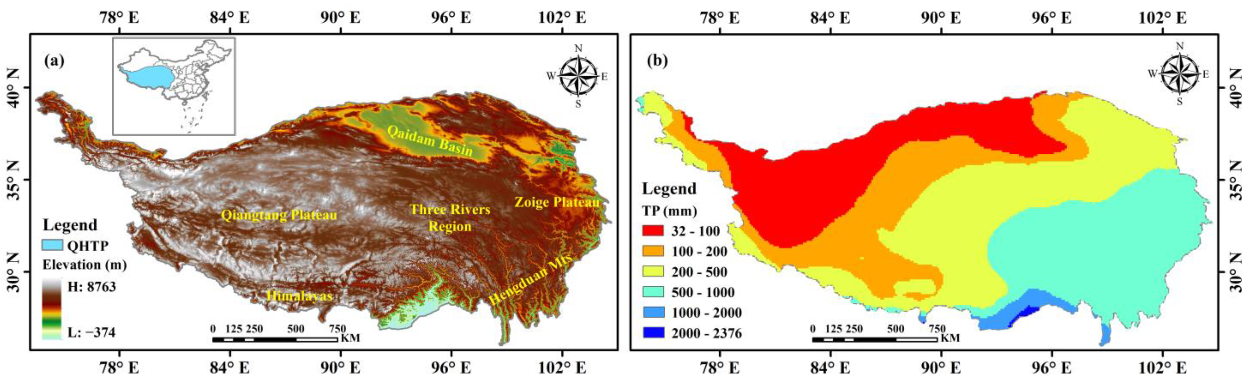
2.1. Study Area

The Tibet Plateau (73°19′~104°47′E, 26°00′~39°47′N) is located in the southwestern part of China, including all of Tibet and parts of Xinjiang, Qinghai, Gansu, Sichuan, and Yunnan. The average altitude of QHTP is above 4000 m and the total area accounts for about 25% of the Chinese mainland (Figure 1a) [39]. As the Asian water tower, QHTP is the birthplace of the Yangtze River, Yellow River, and other rivers, and plays a significant role in water supply and ecosystem security in Asia [40]. It is also one of the most sensitive regions to global climate change, with a considerable increase in the frequency of extremely high temperatures and extreme precipitation in recent years [5]. The unique topography of QHTP makes it form the climate feature with strong radiation, more sunshine, low temperature, and less accumulated temperature, and the temperature decreases with the increase in altitude and latitude. From the spatial distribution of precipitation, we can see that there is a precipitation gradient from northwest to southeast with an obvious increasing trend due to the influence of the South Asian monsoon and westerly winds (Figure 1b). The higher values of precipitation are located southeast of QHTP (>500 mm/a), and the lower values are in the Qaidam Basin and northwest regions (<200 mm/a).

2.2. Data Source

In our study, we selected the monthly (January 1950~December 2014) total precipitation (TP) and PET of version 4 of the Climatic Research Unit gridded time series (CRU) as reference data. The CRU dataset is a 0.5° resolution monthly climate dataset of the global continental surface from 1901 to 2020 produced by the UK National Centre for Atmospheric Science [41]. This dataset is based on a large number of climate anomaly data from meteorological observation stations around the world, and the monthly grid data are established by the angular-distance weight interpolation algorithm. Many comparative studies show that CRU datasets have good applicability in China and the Tibetan Plateau [42,43].

Seven CMIP6 models containing the historical (1950–2014) and future periods (2015–2100) are listed in

Table 1. Information of seven Coupled Model Intercomparison Project (CMIP6) models.

Model	Institution/Country	Grids (lat/lon)	Resolution (km)
AWI-CM-1-1-MR	Alfred Wegener Institute, Germany	192 × 384	100
CMCC-ESM2	Euro-Mediterranean Center on Climate Change, Italy	192 × 288	100
CNRM-CM6-1-HR	National Center for Meteorological Research, France	-	100
FIO-ESM-2-0	First Institute of Oceanography, China	192 × 288	100
GFDL-ESM4	NOAA Geophysical Fluid Dynamics Laboratory, USA	180 × 360	100
INM-CM5-0	Institute of Numerical Mathematics, Russia	120 × 180	100
MRI-ESM2-0	Mitsubishi Research Institute, Japan	160 × 320	100

. The future period includes three scenarios (SSP1-2.6, SSP2-4.5, and SSP5-8.5). Each model contains six variables: precipitation (pr, kg m⁻² s⁻¹), daily maximum near-surface air temperature (tasmax, K), daily minimum near-surface air temperature (tasmin, K), near-surface wind speed (sfcWind, m s⁻¹), surface air pressure (ps, Pa), and surface downwelling shortwave radiation (rsds, W m⁻²). CMIP6 model dataset was downloaded from the Climate Data Store of the European Centre for Medium-Range Weather Forecasts (ECMWF). The spatial resolution of all variables was bilinearly interpolated to 0.1° [44].

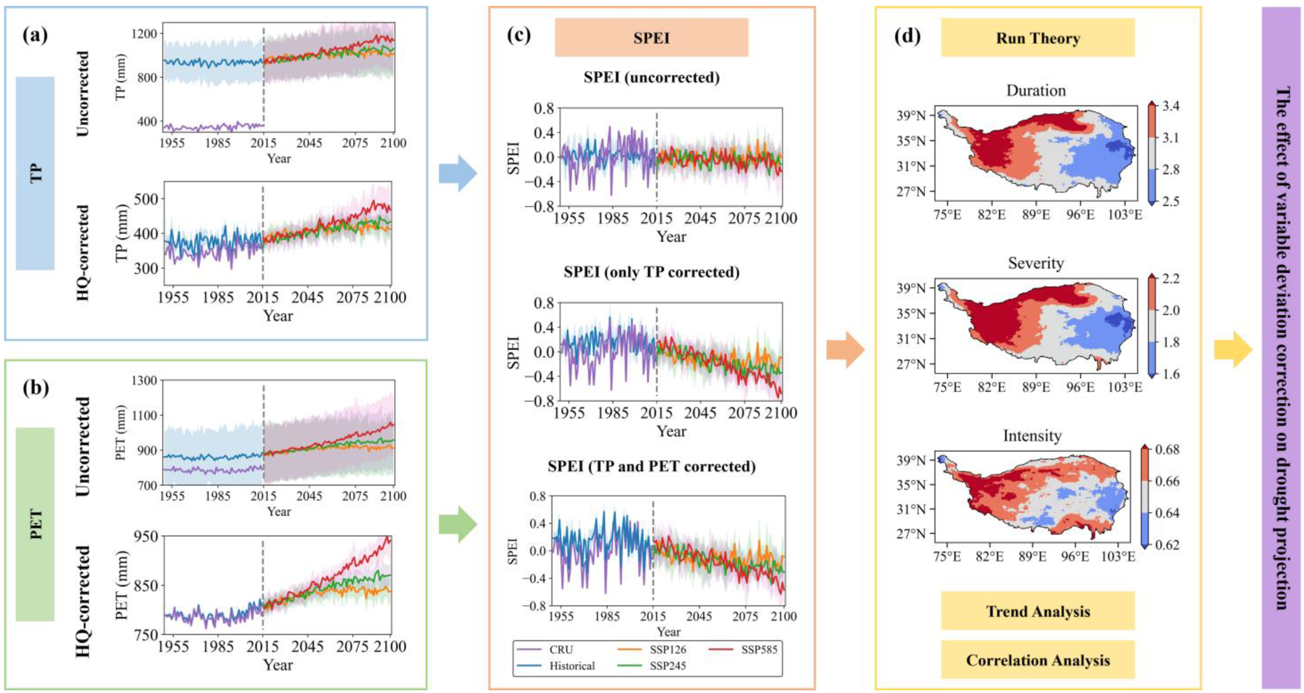
2.3. Methods

The overview of our research flowchart is shown in Figure 2. It is clear from the uncorrected time curve in Figure 2a,b that there is a large systematic deviation (>400 mm) between observed precipitation and simulated data, and a small deviation in PET (<100 mm) Therefore, to improve the accuracy of drought prediction, we added PET correction to the research experiment. First, the precipitation and PET data simulated by the CMIP6 model were corrected. Then, the SPEI drought index and drought characteristics (duration, severity, and intensity) were calculated (Figure 2c,d). Additionally, the effects of correction of precipitation and potential evapotranspiration on drought prediction are discussed and evaluated.

2.3.1. Histogram Matching-Quantile Mapping Correction

Histogram matching, also known as histogram specification, is an operation that transforms the distribution of an image according to a specific mapping mode [45]. It mainly relies on the statistics of the probability density function (PDF) in the spatial dimension and is a commonly used method in image processing [46]. We assume as random variables with PDFs p_a(a) and p_z(z), respectively. Here, a and z denote the intensity levels of the input and output images, respectively. The p_a(a) could be estimated from the given input image, and p_z(z) is the specified PDF that we wish the output image to have. It can be obtained from the reference image. The random variable with the property can be written as:

$$\mathrm{s}=\mathrm{T}\left(\mathrm{a}\right)=\left(\mathrm{L}-1\right){\int }_0^{\mathrm{a}}{\mathrm{p}}_{\mathrm{a}}\left(\mathrm{w}\right)\mathrm{dw}$$

(1)

where w is the dummy variable of integration. L is the intensity of the image level.

Define a function G on variable z with the property:

$$\mathrm{G}\left(\mathrm{z}\right)=\left(\mathrm{L}-1\right){{\displaystyle \int }}_0^{\mathrm{z}}{\mathrm{p}}_{\mathrm{z}}\left(\mathrm{v}\right)\mathrm{dv}=\mathrm{s}$$

(2)

where v is a dummy variable of integration. Hence, the output image could be expressed as:

$$\mathrm{z}={\mathrm{G}}^{-1}\left(\mathrm{s}\right)={\mathrm{G}}^{-1}\left[\mathrm{T}\left(\mathrm{a}\right)\right]$$

(3)

Equation (3) can realize the matching of input and output image histograms.

The QM algorithm has been widely used for variable bias correction in atmospheric science and ecology [16,17]. It establishes a quantile mapping transformation function f(∙) between observation variables P_o and model variables P_m to make their distribution consistent [13]. The transformation can in general be formulated as:

$${\mathrm{P}}_{\mathrm{o}}=\mathrm{f}\left({\mathrm{P}}_{\mathrm{m}}\right)$$

(4)

Further, it can be expressed by using the CDF:

$${\mathrm{P}}_{\mathrm{o}}={\mathrm{F}}_{\mathrm{o}}^{-1}\left({\mathrm{F}}_{\mathrm{m}}\left({\mathrm{P}}_{\mathrm{m}}\right)\right)$$

(5)

where F_m is the CDF of P_m and ${\mathrm{F}}_{\mathrm{o}}^{-1}$ is the inverse CDF of P_o.

In our study, we first conducted the QM correction algorithm for historical and future precipitation and PET with each CMIP6 model. Then, the spatial deviation of the historical period simulated data is calculated by histogram matching, and the multi-year mean value of corresponding months is transmitted to the future monthly data to realize the spatial correction of the future simulated data. The HQ algorithm is performed based on the Python ‘Scikit-image’ library and R package ‘qmap’. We chose the empirical quantiles (QUANT) function in the qmap package, which is a nonparametric transformation method and is more effective to approximate data.

2.3.2. Drought Assessment

SPEI is often used to monitor and assess the occurrence and severity of drought events. We used SPEI as a drought index to evaluate wet and dry conditions over QHTP. The calculation of SPEI requires two variables, precipitation and PET. The PET is calculated using the FAO Penman–Monteith formula [47], which is given by:

$$\mathrm{PET}=\frac{0.408\Delta \left({\mathrm{R}}_{\mathrm{n}}-\mathrm{G}\right)}{\Delta +\mathsf{\gamma }\left(1+0.34{\mathrm{U}}_2\right)}+\frac{\mathsf{\gamma }\frac{900}{\mathrm{T}+273}{\mathrm{U}}_2\left({\mathrm{e}}_{\mathrm{s}}-{\mathrm{e}}_{\mathrm{a}}\right)}{\Delta +\mathsf{\gamma }\left(1+0.34{\mathrm{U}}_2\right)}$$

(6)

where PET is potential evapotranspiration (mm), Δ is slope vapor pressure curve (kPa °C ⁻¹), R_n is net radiation at the crop surface (MJ m⁻² d⁻¹), G is soil heat flux density (MJ m⁻² d⁻¹), γ is psychrometric constant (kPa °C⁻¹), U₂ is the wind speed at 2 m height (m s⁻¹), T is the mean daily air temperature at 2 m height (°C), e_s is saturation vapor pressure (kPa), e_a is actual vapor pressure, e_s – e_a is saturation vapor pressure deficit (kPa).

The difference between precipitation (P) and PET can simply describe the profit and loss of water, the i month can be expressed as:

$${\mathrm{D}}_{\mathrm{i}}={\mathrm{P}}_{\mathrm{i}}-{\mathrm{PET}}_{\mathrm{i}}$$

(7)

The probability density function of a log-logistic distributed variable is expressed as [48]:

$$\mathrm{f}\left(\mathrm{x}\right)={\left[1+{\left(\frac{\mathsf{\alpha }}{\mathrm{x}-\mathsf{\gamma }}\right)}^{\mathsf{\beta }}\right]}^{-1}$$

(8)

where α, β, γ are scale, shape, and origin parameters, respectively [49].

$$\mathrm{SPEI}=\mathrm{W}-\frac{{\mathrm{c}}_0+{\mathrm{c}}_1\mathrm{W}+{\mathrm{c}}_2{\mathrm{W}}^2}{1+{\mathrm{d}}_1\mathrm{W}+{\mathrm{d}}_2{\mathrm{W}}^2+{\mathrm{d}}_3{\mathrm{W}}^3}$$

(9)

where $\mathrm{W}=\sqrt{-2\ln \left(\mathrm{P}\right)}\mathrm{for}\mathrm{P}\le 0.5$, P is the probability of exceeding a determined D_i value. The constants are c₀ = 2.515517, c₁ = 0.802853, c₂ = 0.010328, d₁ = 1.432788, d₂ = 0.189269, d₃ = 0.001308 [50,51]. SPEI-03 is used to characterize short-term meteorological drought in our research. Since the calculation of SPEI depends on the probability distribution of the time series, it is most appropriate to have a time range of at least 30 years.

The indicators for detecting drought events include frequency (F), duration (D), severity (S), and intensity (I) based on the application of run theory [52,53,54]. For a while, the value of SPEI is continuously less than the threshold, which is called a drought event. This period is called duration, and the cumulative intensity of the drought is called the severity throughout the drought [6]. The duration, severity, and intensity of the drought in this article are for all drought events counted on pixels. Using the Penman function and SPEI function from the R ‘SPEI’ package, we compute PET and SPEI for historical and future scenarios. The drought threshold of SPEI is −0.5, a threshold of ‘Abnormally dry’ used by the U.S. Drought Monitor [44].

2.3.3. Correlation, Trend Analysis

Pearson’s correlation coefficient is a method commonly used to measure the degree of linear correlation between two groups of data [55]. It can be seen as eliminating the dimensional influence of two variables, that is, the covariance after normalizing of two variables. The larger the absolute value of the correlation coefficient, the stronger the correlation. It is mainly applicable to three situations: (1) the relationship between the two variables is linear; (2) the totality of the two variables is normal; (3) the observations of the two variables appear in pairs, and the observations are independent of each other. This study uses it to compute the correlation between the CMIP6 model and the CRU dataset.

The Mann–Kendall trend test is a nonparametric test used to analyze time series data for a persistent increasing or decreasing trend [56]. It has the following advantages: (1) it is not assumed that the data are distributed according to a specific rule; (2) it is not affected by missing data; (3) it is not affected by irregular data intervals and is not affected by the length of time series [57,58]. This study uses this approach to analyze precipitation, PET, and SPEI trends relative to historical and future scenarios.

3. Results

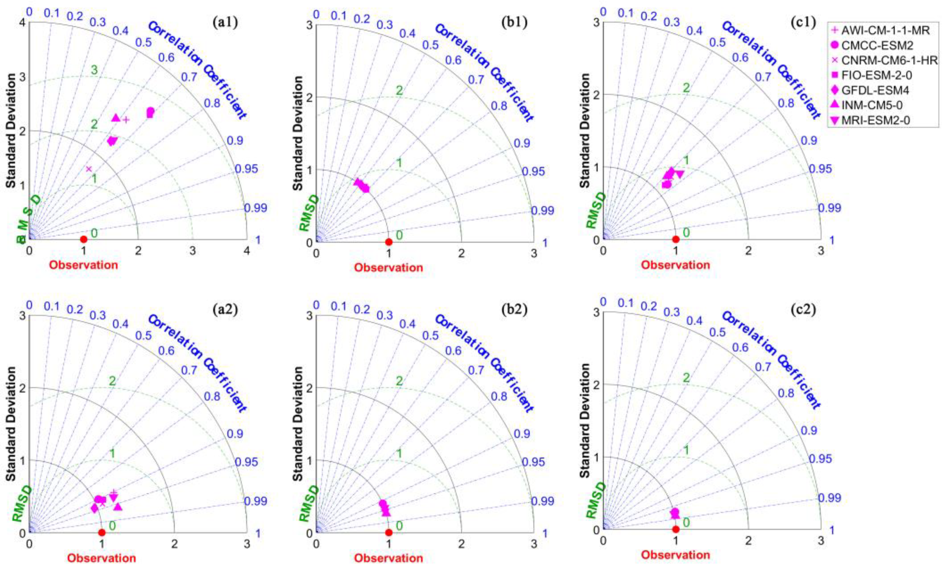
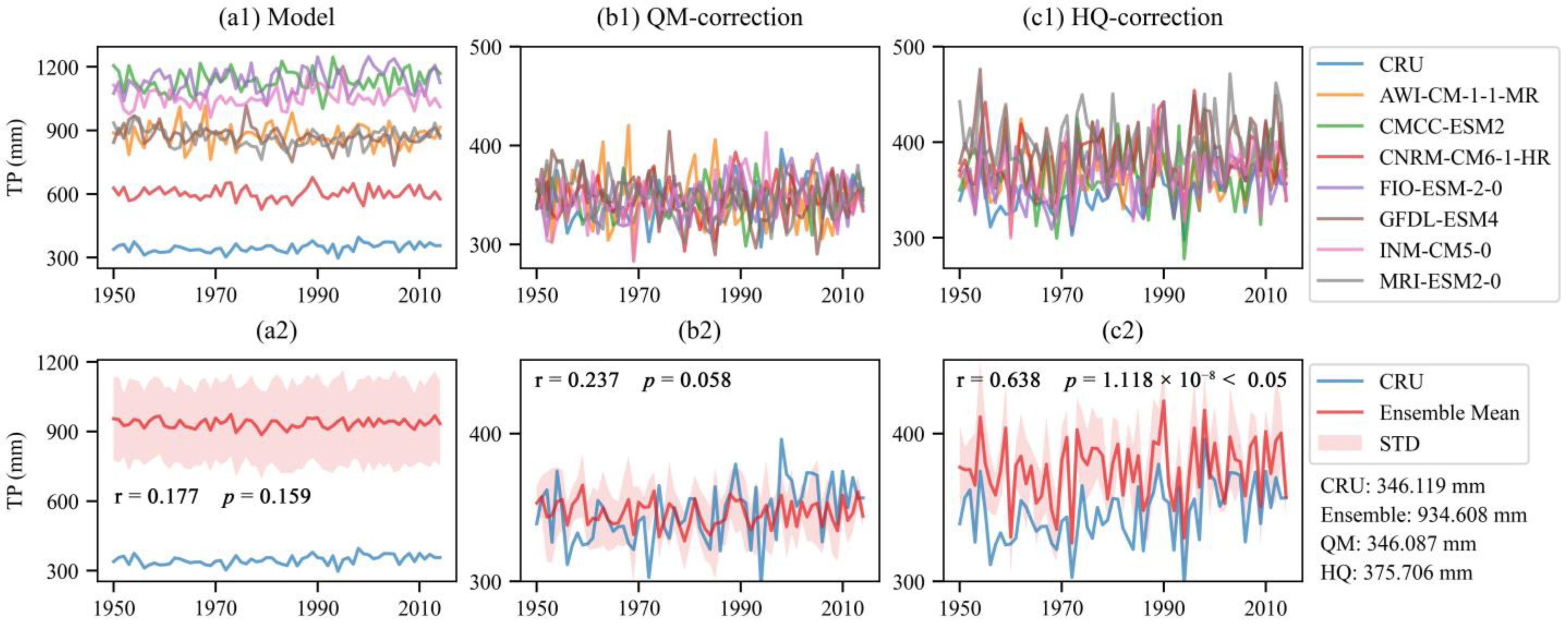
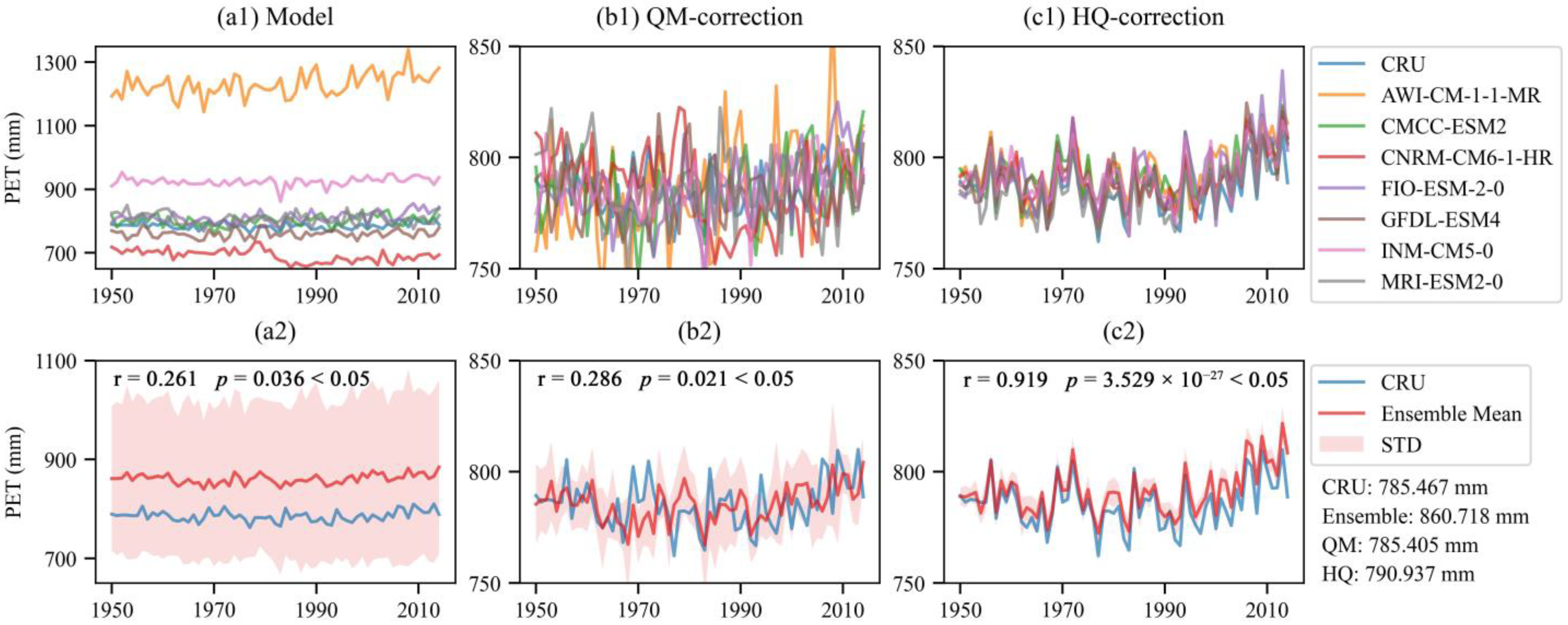
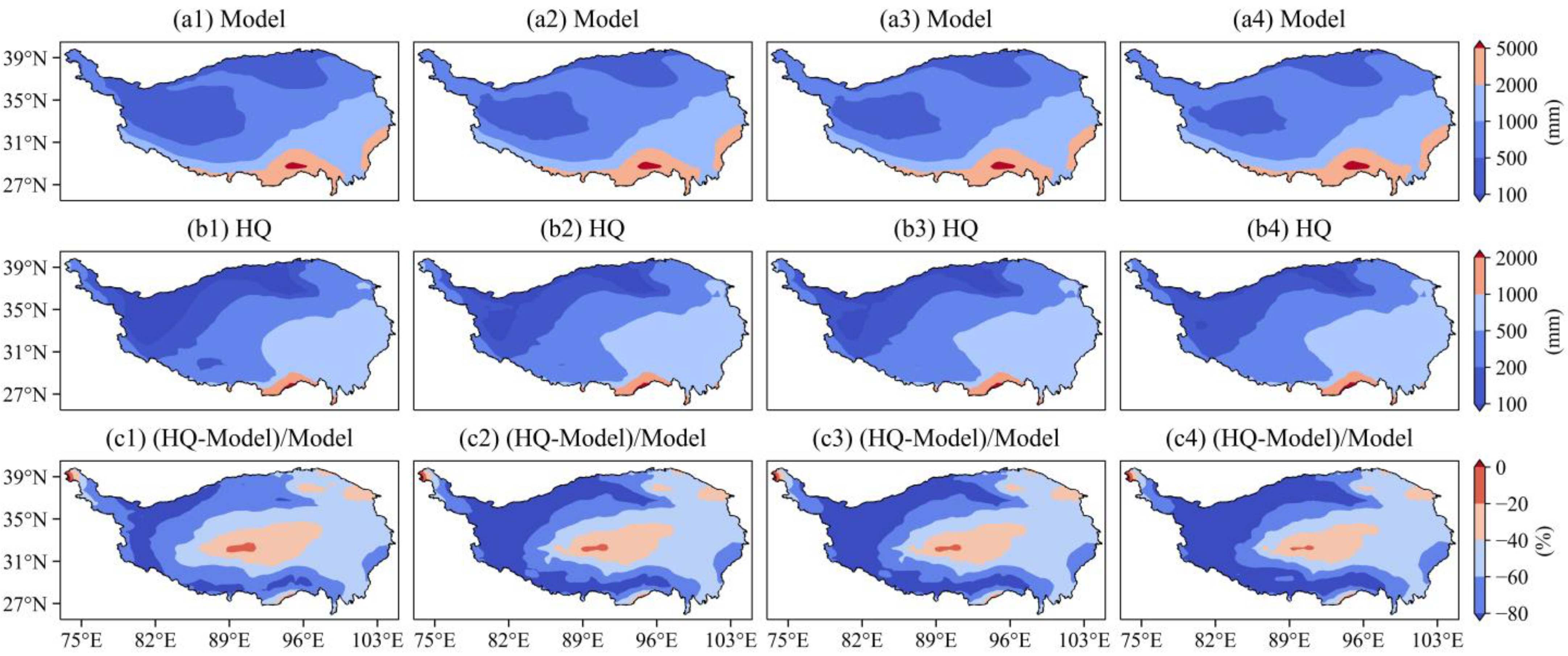
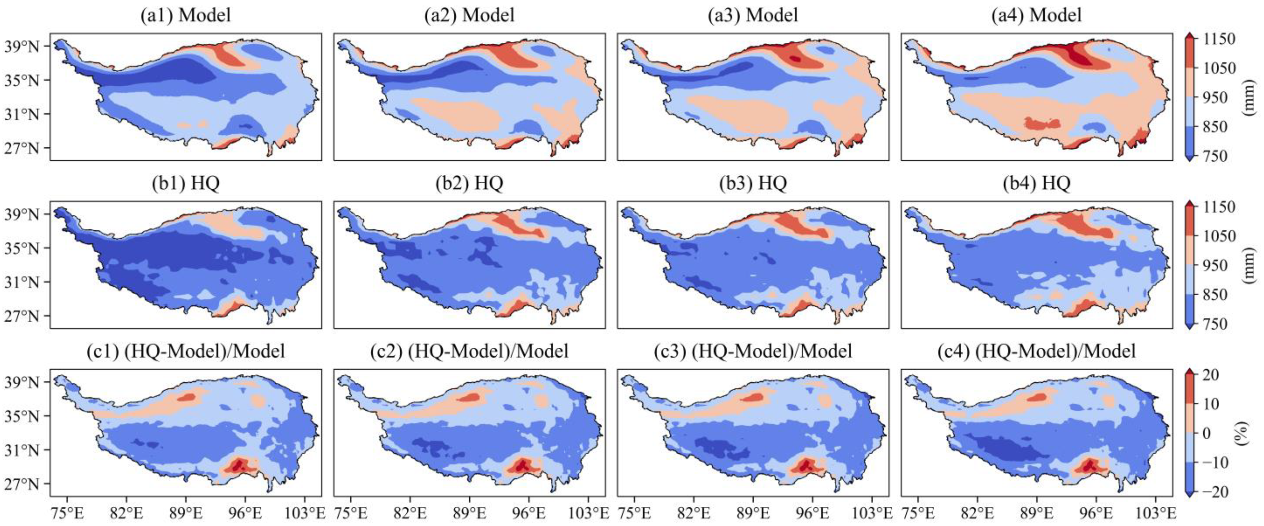
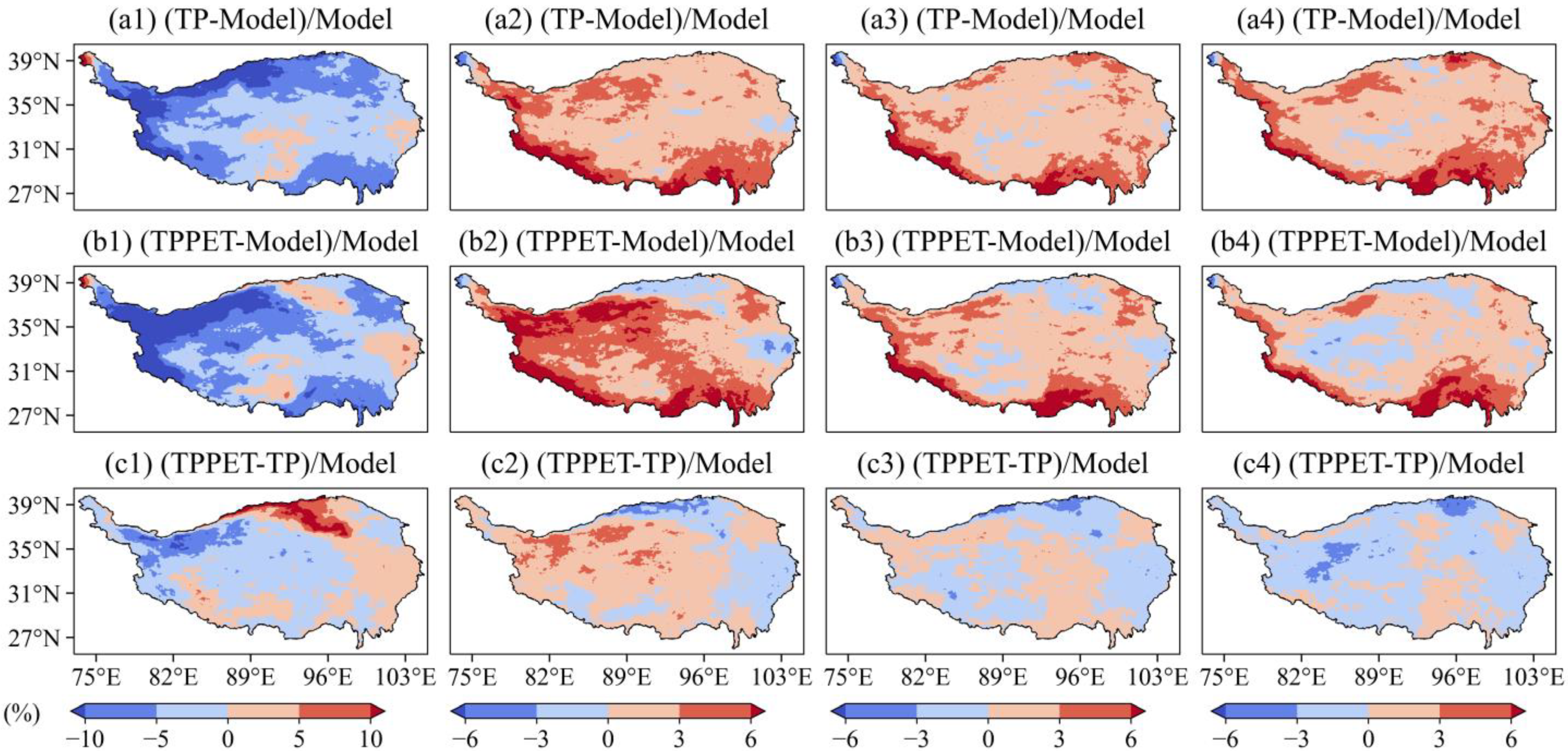
3.1. Proof of Spatiotemporal HQ-Corrected Method Effectiveness

To evaluate the accuracy of the correction results, we first calculated the correlation coefficient (R), standard deviation (STD), and root mean square error (RMSE) between seven CMIP6 models and CRU datasets. The standardized Taylor diagrams as displayed in Figure 3, were then made by averaging the three indicators in the QHTP zone. The simulation capability of the model in the historical period can be accurately expressed using the standardized Taylor diagrams. The STD and RMSE of most uncorrected models are maintained above 2.0, while the R of precipitation is often over 0.5. After QM correction, the model’s STD and RMSD are significantly decreased (by roughly 1.0), but R is not significantly enhanced. Although STD has slightly increased after HQ adjustment, the range of the correlation coefficient has grown from 0.5~0.7 to 0.7~0.8. Seven CMIP6 models had a better ability to simulate PET than precipitation, with R above 0.9 and STD maintained at roughly 1.0. The range of the R of 7 models rises from 0.9~0.95 to 0.95~0.99. after HQ correction. In general, the simulation accuracy of precipitation and PET of seven CMIP6 models after HQ correction is generally closer to that of the CRU observation data. To further demonstrate the effectiveness of HQ correction in the spatiotemporal dimension, the changes in precipitation and PET over the temporal dimension are shown in Figure 4 and Figure 5. The precipitation of 7 CMIP6 models is generally higher than that of the CRU observation data (Figure 4(a1)). The observed annual TP is 346.119 mm, whereas the ensemble average annual TP is 934.608 mm (Figure 4(a2)). Despite the ensemble simulation’s mean dropping to 346.087 mm after QM correction, the correlation with the observed data was weak and failed to meet the criteria for statistical significance (r = 0.237, p = 0.058) (Figure 4(b2)). PET is in a similar condition. The simulated data from CMCC-ESM2, FIO-ESM-2-0, GFDL-ESM4, and MRI-ESM2-0 are comparable to the observation data from CRU in the uncorrected simulated data (Figure 5(a1)). After QM correction, the correlation coefficient increased from 0.261 to 0.286, but the p-value were not assessed for significance (r = 0.261, p = 0.036; r = 0.286, p = 0.021) (Figure 5(a2,b2)). HQ correction further corrects the spatial distribution deviation, which improves the similarity of precipitation and PET ensemble model simulation to a certain extent (r = 0.638, p = 1.118 × 10⁻⁸; r = 0.919, p = 3.529 × 10⁻²⁷) (Figure 4(c3) and Figure 5(c3)). The spatial correlation and statistics are shown in Figures S1 and S2, Tables S1 and S2, which can also indirectly reflect that HQ correction improves the spatial simulation ability of the marginal region with low correlation.

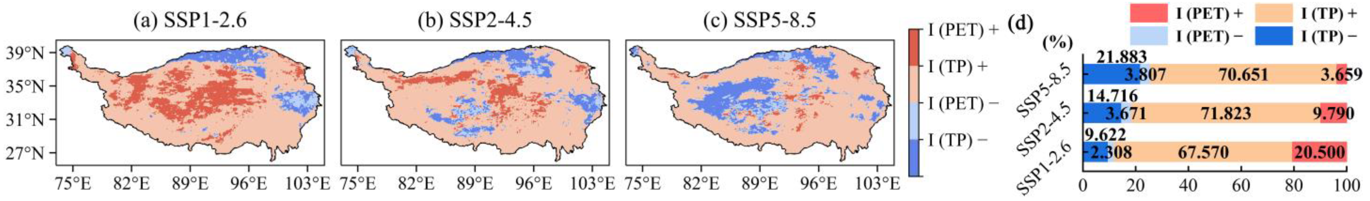
3.2. Quantifying the Impact of Precipitation and PET Correction on Drought Projection

To quantify the impact of precipitation and PET correction on drought features, we initially quantified the spatial changes of variables before and after correction, as shown in Figure 6 and Figure 7. The corrected precipitation level lowers slightly but does not alter the spatial structure of the precipitation gradient zone, and the difference between the multi-year precipitation and the corrected value under the historical and future scenarios has a strong spatial consistency. According to Figure 7(b1–b4), rainfall is higher in southeast Tibet (>1000 mm) and lower in parched northwest Tibet (<200 mm). The correction percentages are less than zero in the majority of places, forming a C-shape around the Qiangtang Basin with a higher exterior (<−60%) and a lower basin (>−40%) (Figure 7(c1–c4)). The spatial pattern of potential evapotranspiration is different from that of precipitation, With high values primarily spread in the Qaidam Basin and southern Tibet (>1050 mm) and low values primarily distributed in the northwestern Plateau (<850 mm). The corrected value of PET, which has a narrower variable range than precipitation, notably increased in southern Tibet and northern Tibet (>0%), while decreasing in the majority of other locations (<0%). The spatial distribution of correction values of historical and future scenarios is consistent.

Then, we estimated three different forms of SPEI, including SPEI (uncorrected), SPEI (only TP corrected), and SPEI (TP and PET corrected) based on the run theory. Figure 8 depicts the feature of intensity, whereas Figures S3–S6 depict the features of frequency, duration, and severity in historical and future scenarios. When compared to the future scenario, the average drought severity of a single occurrence in the historical scenario varies from 0.50 to 062, while it rises to 0.62~0.68 (Figure 8). Along with drought intensity, individual drought event duration and severity have also gotten longer and worse. We quantified the distinction between the three types of drought intensity, as shown in Figure 9, to more thoroughly investigate how drought intensity changed over the repair process. In Figures S7–S10, the frequency, duration, and severity characteristics are displayed. The three different types, respectively, represent three meanings. Intensity ((TP-Model)/Model) can be regarded as the intensity change only caused by the deviation correction of precipitation, Intensity ((TPPET-Model)/Model) is the intensity change caused by the common deviation correction of precipitation and PET. Intensity ((TPPET-TP)/Model) refers to the intensity change only caused by the deviation correction of PET. The intensity changes brought on by precipitation and PET correction are very consistent with the intensity changes brought on by precipitation alone when comparing the regional distribution under historical and future scenarios. The frequency, duration, and severity of droughts were distributed spatially with the same characteristics.

The primary drivers of drought intensity change in future scenarios were finally identified by the change in drought intensity induced by precipitation and PET correction, as shown in Figure 10. The highest (minimum) value of the rise (reduction) in intensity ((TP-Model)/Model) and intensity ((TPPET-TP)/Model) in this pixel is chosen to establish the primary driving element when drought intensity increases ((TPPET-Model)/Model) (or drops). Combining the statistical findings, the regions with growing drought intensity accounted for 88.070%, 81.613%, and 74.310%, whereas the areas with decreasing drought intensity accounted for 11.930%, 18.387%, and 25.690%, respectively (Figure 10d). A balance of around 70.015% and 3.262% was maintained between the intensity increase caused by precipitation and the intensity drop caused by PET. The region of intensity rise dominated by PET reduced from 20.500% to roughly 3.659%, and the area of intensity decrease dominated by precipitation rose from 9.622% to 21.883%. In combination with the correction of multi-year mean values of precipitation and PET mentioned above, we counted the variation amount and area of precipitation, PET, and drought intensity in three future scenarios (

Table 2. Statistics of spatial correction results in future scenarios (+ or − indicates the increase or decrease in variable and R is the area ratio).

	TP				PET				Drought Intensity
(%)	+	R	−	R	+	R	−	R	+	R	−	R
SSP1-2.6	6.470	0.048	−63.098	99.952	5.827	12.488	−10.405	87.512	3.785	88.070	−1.375	11.930
SSP2-4.5	6.622	0.048	−63.535	99.952	5.868	12.058	−10.729	87.942	2.435	81.613	−1.039	18.387
SSP5-8.5	6.428	0.048	−66.152	99.952	5.948	11.161	−11.450	88.839	2.405	74.310	−1.003	25.690
Mean	6.507	0.048	−64.262	99.952	5.881	11.902	−10.861	88.098	2.875	81.331	−1.139	18.669

). The yearly TP was reduced by 64.262% as a result of the adjusted precipitation decreasing in 99.952% of locations of the QHTP. After correction, the PET of 11.902 areas increased with a 5.881% annual PET rise; the potential evapotranspiration of 88.098% of areas declined with a 10.861% yearly PET reduction. In addition, a single drought event’s intensity rose in 81.331% of regions by 2.875% and fell in 18.669% of regions by 1.139%.

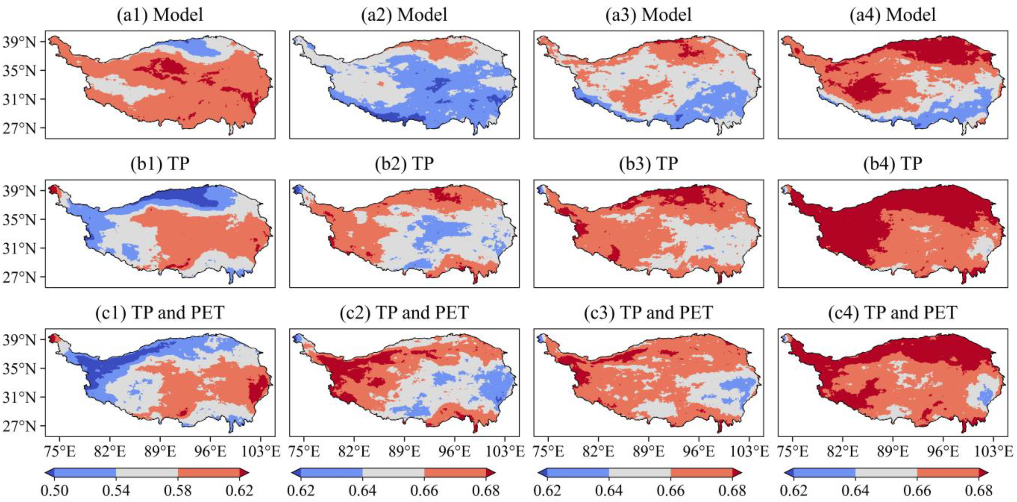
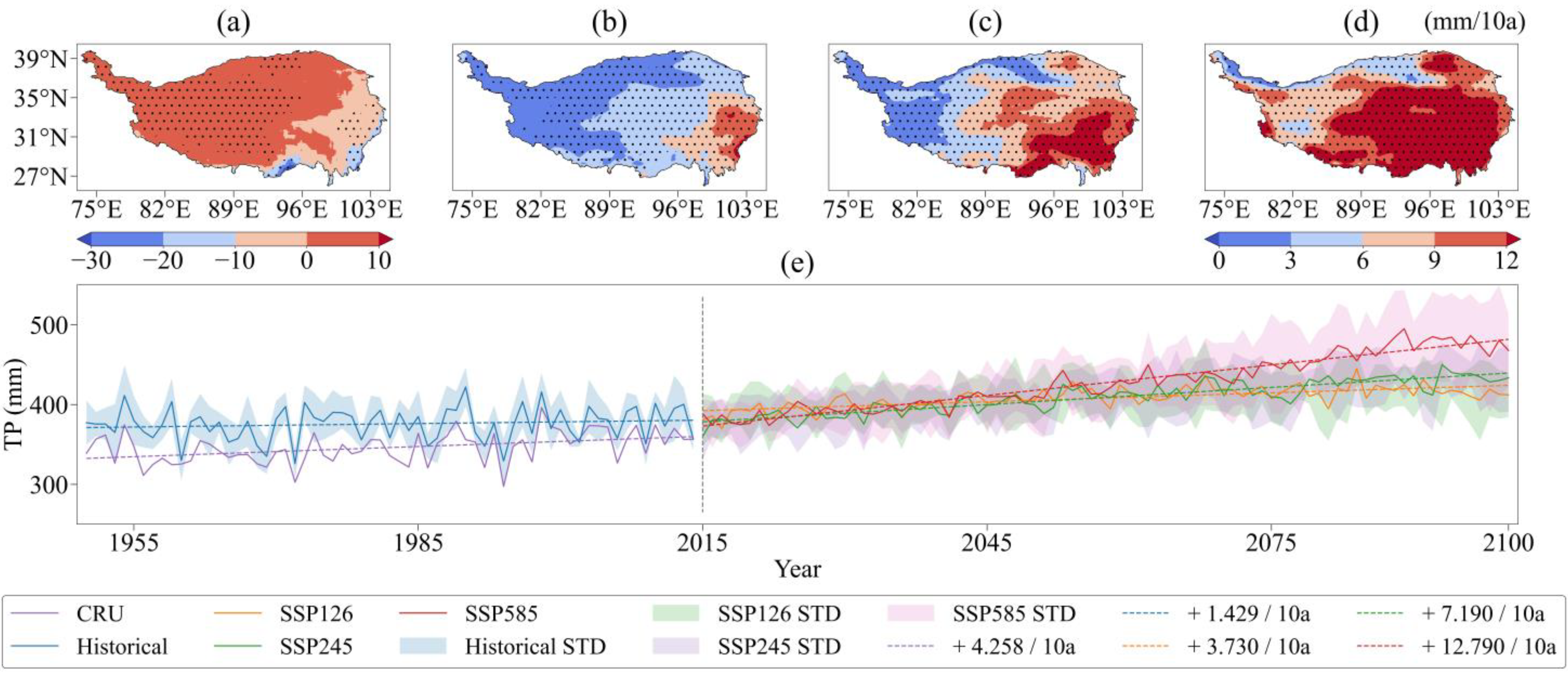
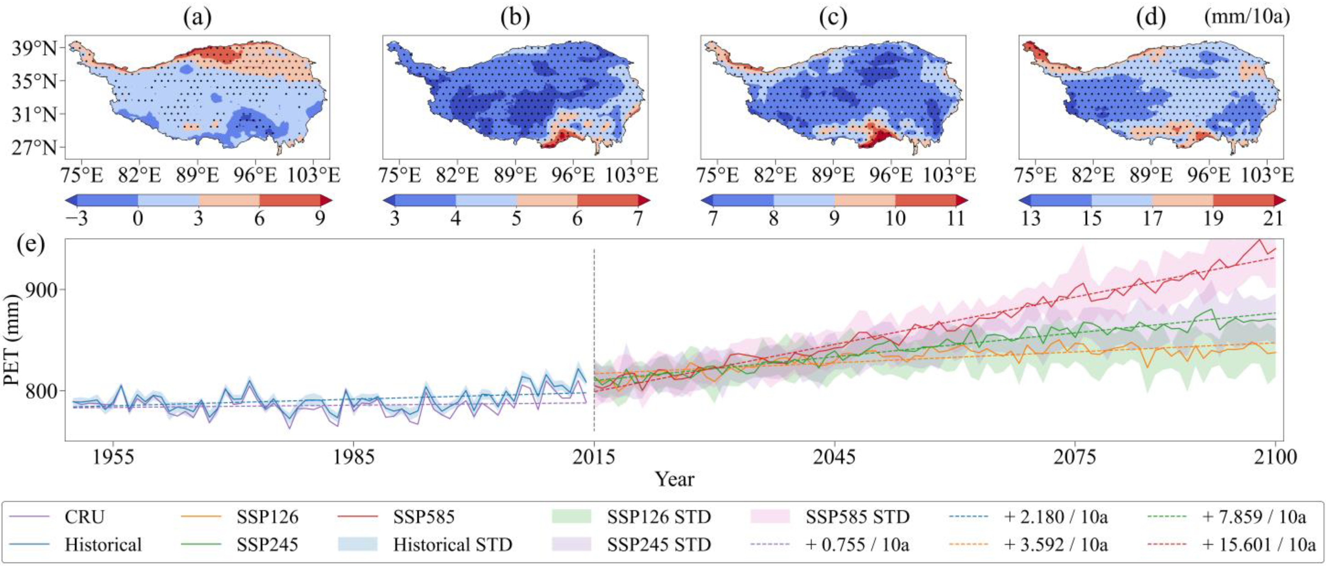
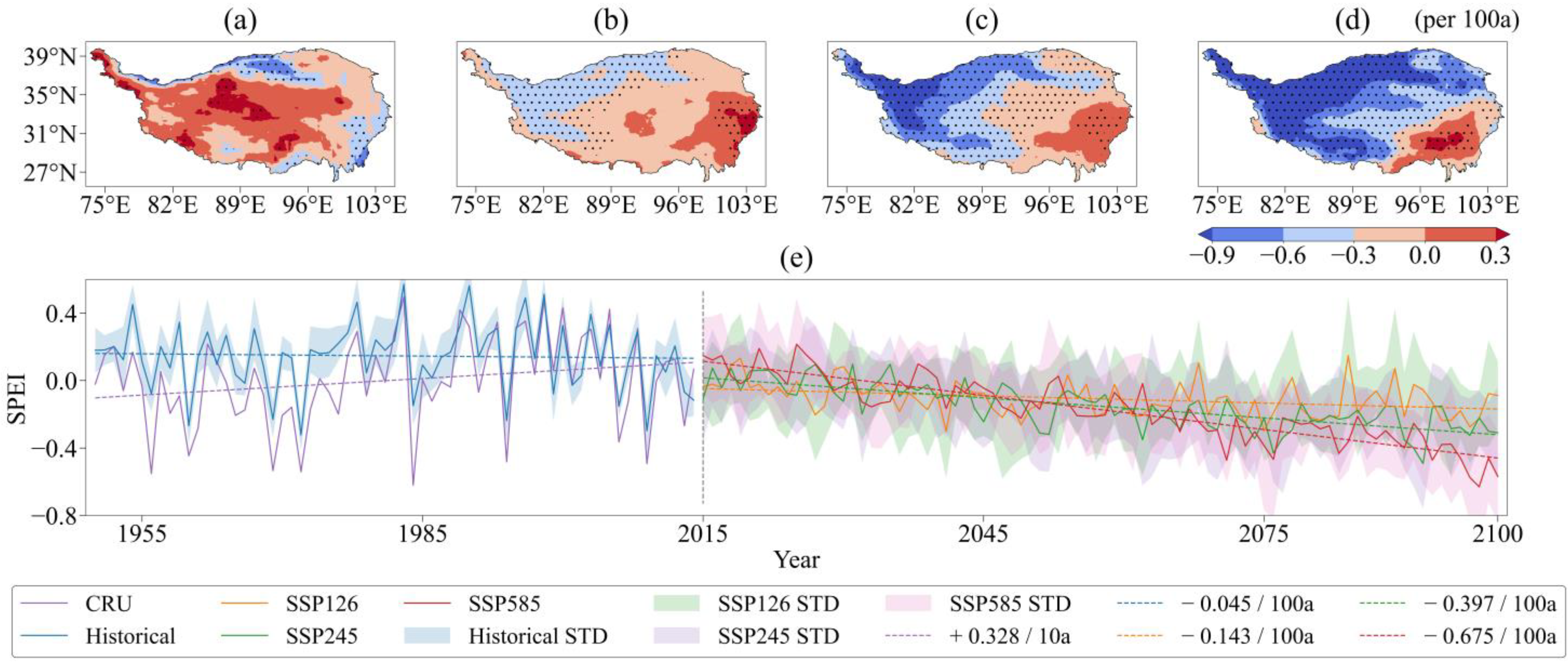
3.3. Future Trend Changes and Significance of Precipitation, PET, and SPEI

We analyzed trends in TP, PET, and SPEI in historical and future scenarios of the ensemble model using the Mann–Kendall trend test. The trends of the original and HQ-corrected ensemble model in the spatial and temporal dimensions of precipitation are shown in Figure S11 and Figure 11. The historical precipitation trend showed an increasing pattern from southeast to northwest in space. The precipitation trend in the future scenario had a higher growth rate in the southeast than in the northwest. As the scenario increases, the growth rate gradually increased. The growth rates of the future scenarios for the original ensemble model were 7.594 mm/10a, 15.017 mm/10a, and 27.377 mm/10a; for the HQ-corrected ensemble model were 3.730 mm/10a, 7.190 mm/10a, and 12.790 mm/10a, respectively. The trends of the original and HQ-corrected ensemble model in the spatial and temporal dimensions of PET are shown in Figure S12 and Figure 12. The growth rates of the future scenarios for the original ensemble model were 4.227 mm/10a, 9.665 mm/10a, and 19.561 mm/10a; for the HQ-corrected ensemble model were 3.592 mm/10a, 7.859 mm/10a, and 15.601 mm/10a, respectively.

The trends of the SPEI (uncorrected), SPEI (only TP corrected), and SPEI (TP and PET corrected) ensemble models in the spatial and temporal dimensions are shown in Figures S13 and S14, and Figure 13. The spatial distribution of SPEI trends of the three ensemble models was almost identical. The region with a growth rate larger than 0 is located in the northern Tibet Plateau under the historical scenario, but with the alteration of the future scenario, it is moved to the southeast of Tibet. The SPEI in southeast Tibet has a clear increasing trend under the SSP5-8.5 scenario, but the SPEI in other regions has a major decrease trend, and there is a clear split zone. The growth rates of the historical and future scenarios for the SPEI (uncorrected) ensemble model were −0.033/100a, 0.047/100a, −0.056/100a, and −0.133/100a; for the SPEI (only TP corrected) ensemble model −0.007/100a, 0.179/100a, −0.492/100a, and −0.862/100a; and for the SPEI (TP and PET corrected) ensemble model −0.045/100a, −0143/100a, −0.397/100a, and −0.675/100a, respectively.

4. Discussion

4.1. The Impact of Precipitation and PET Correction on Drought Assessment

The mean value of precipitation observed by the CRU data is 346.119 mm, which is comparable to previous research [59]. The difference between the CRU precipitation and the ensemble CMIP6 precipitation is 588.489 mm (Figure 4(a2)). The distinction between ensemble PET data and CRU PET data (within the range of standard deviation) is 75.251 mm. Due to this, some of the current drought estimates only correct for precipitation bias without correcting for PET [44]. Therefore, Precipitation should thus be the primary factor impacting the accuracy of drought assessment across the QHTP from the standpoint of basic data deviation. It is clear from comparing the three forms of SPEI change curves that SPEI (only TP corrected) change will be far less than that of SPEI (uncorrected). For example in the SSP5-8.5 scenario, precipitation deviation adjustment causes the changing trend to shift from −0.133/100a to −0.862/100a (Figures S13 and S14). After the correction of SPEI (TP and PET corrected) was estimated, the overall plummeting rate was eased and increased from −0.862/100a to −0.675/100a. From the standpoint of the drought index, this SPEI trend can also demonstrate the impact of precipitation variance on drought evaluation. We looked at it in terms of the main drivers from a spatial viewpoint (Figure 10a–c), the majority of regions are seeing a rise in drought severity. The area of decreasing drought intensity caused by decreasing precipitation is expanding, while the area of increasing drought intensity caused by increasing PET is shrinking. The intensity rise led by PET gradually changed to the intensity drop trend led by precipitation in the northern Tibet region, while the intensity decrease trend led by precipitation gradually changed to the intensity increase trend in the Zoige area. As a result, future changes in drought intensity will be dominated by changes in precipitation. As shown in Table 2, the correction reduced 64% of the total precipitation over the QHTP and 11% of the PET in 88% of the region, and increased 6% of the PET in 12% of the region, resulting in a 3% increase in the drought intensity in 81% of the QHTP and a 1% decrease in the drought intensity in 19% of the region.

4.2. The Relationship between Future Precipitation, PET, and SPEI Changes

By comparing the precipitation before and after correction, we found that the growth rate in the future scenario was overestimated, but the spatial pattern did not change greatly. The spatial trend of precipitation is consistent with other works [37,60]. With the increase in the scenario, the increasing trend of precipitation in southeast Tibet was significantly enhanced, and the growth rate decreased from southeast to northwest. Compared with the SPEI trend before and after correction, the uncorrected simulation results underestimated the downward trend of SPEI in the future scenario, and the overall spatial pattern did not change significantly. The SPEI growth rate is more than 0 in some parts of southeast Tibet and less than 0 in other parts of northwest Tibet. This feature is more and more obvious in the SSP5-8.5 scenario [34]. Why does this feature exist? The reason should also be attributed to the combined effect of precipitation and PET changes. We first analyzed the original uncorrected precipitation, potential evapotranspiration, and SPEI results under the SSP5-8.5 scenario. In the region with a growth rate of SPEI greater than 0, the precipitation growth rate is higher but the potential evapotranspiration growth rate is lower. SPEI is the result of the joint action of precipitation and PET. If the SPEI growth rate remains unchanged, the growth rate of precipitation and PET should maintain a certain balance, and the change in the SPEI growth rate is the result of the imbalance of this balance. Therefore, the actual growth rate of precipitation is greater than the growth rate required for equilibrium, which makes precipitation accumulate and the climate becomes humid, so the SPEI growth rate is greater than 0. The increase in soil moisture led to an upward trend in SPEI. The historical study also shows that the drought in southeastern QHTP has a significant wet trend [32]. The future ecological risk gradually decreases from northwest to southeast [61]. Therefore, the above factors will make the SPEI trend in southeastern QHTP.

4.3. Limitation and Future Research

Although the impact of precipitation correction on drought estimation has been quantified and the future changes in precipitation and SPEI on QHTP have been analyzed, there are still certain limitations in methods and research. In terms of the method [18], the HQ method assumes that the deviation is stationary in the future and the deviation of the spatial correction is passed to the future by calculating the mean value of each month in the historical correction. This assumption is challenged by the notion that future variances are characterized by non-stationary trends [62,63]. Regardless of non-stationarity and trend, most statistical methods for bias correction do not take into account the physical mechanisms between variables and model simulations [64]. Therefore, the study of future methods should not only consider the correction between multivariate but also pay attention to the physical mechanism of simulation bias [65]. HQ correction will change the future trend to a certain extent. Some studies believe that the future forecast trend is biased, but others believe that the future forecast variability is credible. These factors need to be further considered in future studies.

In terms of basic data, seven CMIP6 models with higher resolution and more comprehensive data were selected in this paper to predict future drought changes. More global or regional simulation models with higher precision and spatial resolution should be selected in the future. SPEI is a drought accumulation index based on probability distribution. In the process of calculating SPEI based on precipitation and potential evapotranspiration, the influence of precipitation and potential evapotranspiration correction on drought prediction cannot be measured by variability. In future research on model simulation, it is necessary not only to study the model with higher simulation accuracy but also to establish a new linear or nonlinear relationship between the drought index and the basic variables, to fully understand how the change of precipitation affects the change of drought.

5. Conclusions

This study investigated the influence of precipitation deviation correction on drought prediction using data from seven CMIP6 model simulations and CRU observational data. The findings indicate that the annual total precipitation throughout the majority of the Qinghai–Tibet Plateau would fall by 64.262% through HQ correction in the future scenario. Additionally, there are deviations in the projection of future precipitation and SPEI trends. The following are the primary conclusions:

(1)

The spatiotemporal HQ correction approach may successfully increase the simulation accuracy of the integrated model using the Taylor diagram and spatiotemporal analysis. The correlation with observed precipitation rose from 0.237 (p = 0.058) to 0.638 (p = 1.118 × 10⁻⁸) when compared with QM correction, and the correlation with observed PET increased from 0.286 (p = 0.021) to 0.919 (p = 3.529 × 10⁻²⁷).

(2)

The change of drought intensity over the QHTP in the future is mainly controlled by precipitation correction, with the area accounting for 85.422%. The average annual total precipitation in the 99.952% region declined by 64.262% and the average annual total PET in the 11.902% area had a rise of 5.881%, and the 88.098 regions saw a loss of 10.861% with HQ correction. When fundamental factors were corrected, the intensity of a single drought event rose in the 81.331% region by 2.875% and dropped in the 18.669% area by 1.139%.

(3)

The original ensemble model overestimates the increasing trend of precipitation and underestimates the decreasing trend in SPEI in three future scenarios. The rate of precipitation growth increases from 7.594 mm/10a, 15.017 mm/10a, and 27.377 mm/10a to 3.730 mm/10a, 7.190 mm/10a, and 12.790 mm/10a after HQ correction, correspondingly. The downward trend in SPEI changed from 0.047/100a, −0.056/10a, and −0.133/10a to −0.143/100a, −0.397/100a, and −0.6675/100a.

Our focus is on quantifying the impact of precipitation correction on drought prediction because there are significant uncertainties in precipitation modeling. This can obtain a more reliable method for future drought projection, and assessing drought characteristics can help with decision-making for drought management and mitigation.

References

- Solomon, S.; Qin, D.; Manning, M.; Averyt, K.; Marquis, M. Climate Change 2007—The Physical Science Basis: Working Group I Contribution to the Fourth Assessment Report of the IPCC; Cambridge University Press: Cambridge, UK, 2007; Volume 4. [Google Scholar]
- Trenberth, K.E.; Dai, A.; Van Der Schrier, G.; Jones, P.D.; Barichivich, J.; Briffa, K.R.; Sheffield, J. Global warming and changes in drought. Nat. Clim. Chang. 2014, 4, 17–22. [Google Scholar] [CrossRef]
- Arias, P.; Bellouin, N.; Coppola, E.; Jones, R.; Krinner, G.; Marotzke, J.; Naik, V.; Palmer, M.; Plattner, G.-K.; Rogelj, J. Climate Change 2021: The Physical Science Basis. Contribution of Working Group14 I to the Sixth Assessment Report of the Intergovernmental Panel on Climate Change; Technical Summary; 2021. Available online: https://www.ipcc.ch/report/sixth-assessment-report-working-group-i/ (accessed on 15 August 2022).
- Gu, L.; Chen, J.; Yin, J.; Xu, C.Y.; Zhou, J. Responses of precipitation and runoff to climate warming and implications for future drought changes in China. Earth’s Future 2020, 8, e2020EF001718. [Google Scholar] [CrossRef]
- Yong, Z.; Xiong, J.; Wang, Z.; Cheng, W.; Yang, J.; Pang, Q. Relationship of extreme precipitation, surface air temperature, and dew point temperature across the Tibetan Plateau. Clim. Chang. 2021, 165, 41. [Google Scholar] [CrossRef]
- Ukkola, A.M.; De Kauwe, M.G.; Roderick, M.L.; Abramowitz, G.; Pitman, A.J. Robust future changes in meteorological drought in CMIP6 projections despite uncertainty in precipitation. Geophys. Res. Lett. 2020, 47, e2020GL087820. [Google Scholar] [CrossRef]
- Huang, D.Q.; Zhu, J.; Zhang, Y.C.; Huang, A.N. Uncertainties on the simulated summer precipitation over Eastern China from the CMIP5 models. J. Geophys. Res. Atmos. 2013, 118, 9035–9047. [Google Scholar] [CrossRef]
- Chai, Y.; Yue, Y.; Slater, L.J.; Yin, J.; Borthwick, A.G.; Chen, T.; Wang, G. Constrained CMIP6 projections indicate less warming and a slower increase in water availability across Asia. Nat. Commun. 2022, 13, 4124. [Google Scholar] [CrossRef] [PubMed]
- Ficklin, D.L.; Abatzoglou, J.T.; Robeson, S.M.; Dufficy, A. The influence of climate model biases on projections of aridity and drought. J. Clim. 2016, 29, 1269–1285. [Google Scholar] [CrossRef]
- Johnson, F.; Sharma, A. What are the impacts of bias correction on future drought projections? J. Hydrol. 2015, 525, 472–485. [Google Scholar] [CrossRef]
- Cannon, A.J.; Sobie, S.R.; Murdock, T.Q. Bias correction of GCM precipitation by quantile mapping: How well do methods preserve changes in quantiles and extremes? J. Clim. 2015, 28, 6938–6959. [Google Scholar] [CrossRef]
- Piani, C.; Weedon, G.; Best, M.; Gomes, S.; Viterbo, P.; Hagemann, S.; Haerter, J. Statistical bias correction of global simulated daily precipitation and temperature for the application of hydrological models. J. Hydrol. 2010, 395, 199–215. [Google Scholar] [CrossRef]
- Gudmundsson, L.; Bremnes, J.B.; Haugen, J.E.; Engen-Skaugen, T. Downscaling RCM precipitation to the station scale using statistical transformations–a comparison of methods. Hydrol. Earth Syst. Sci. 2012, 16, 3383–3390. [Google Scholar] [CrossRef]
- Song, Z.; Xia, J.; She, D.; Li, L.; Hu, C.; Hong, S. Assessment of meteorological drought change in the 21st century based on CMIP6 multi-model ensemble projections over mainland China. J. Hydrol. 2021, 601, 126643. [Google Scholar] [CrossRef]
- Sian, K.T.C.L.K.; Hagan, D.F.T.; Ayugi, B.O.; Nooni, I.K.; Ullah, W.; Babaousmail, H.; Ongoma, V. Projections of Precipitation Extremes based on Bias-corrected CMIP6 Models Ensemble over Southern Africa. Int. J. Climatol. 2022, 1–21. [Google Scholar] [CrossRef]
- Ngai, S.T.; Juneng, L.; Tangang, F.; Chung, J.X.; Salimun, E.; Tan, M.L.; Amalia, S. Future projections of Malaysia daily precipitation characteristics using bias correction technique. Atmos. Res. 2020, 240, 104926. [Google Scholar] [CrossRef]
- Tong, Y.; Gao, X.; Han, Z.; Xu, Y.; Xu, Y.; Giorgi, F. Bias correction of temperature and precipitation over China for RCM simulations using the QM and QDM methods. Clim. Dyn. 2021, 57, 1425–1443. [Google Scholar] [CrossRef]
- Nahar, J.; Johnson, F.; Sharma, A. Addressing spatial dependence bias in climate model simulations—An independent component analysis approach. Water Resour. Res. 2018, 54, 827–841. [Google Scholar] [CrossRef]
- Hannachi, A.; Jolliffe, I.T.; Stephenson, D.B. Empirical orthogonal functions and related techniques in atmospheric science: A review. Int. J. Climatol. A J. R. Meteorol. Soc. 2007, 27, 1119–1152. [Google Scholar] [CrossRef]
- Yu, H.; Zhang, Q.; Wei, Y.; Liu, C.; Ren, Y.; Yue, P.; Zhou, J. Bias-corrections on aridity index simulations of climate models by observational constraints. Int. J. Climatol. 2022, 42, 889–907. [Google Scholar] [CrossRef]
- Nanjegowda, R.A.; Parambath, S.K. A novel bias correction method for extreme rainfall events based on L-moments. Int. J. Climatol. 2022, 42, 250–264. [Google Scholar] [CrossRef]
- Hannachi, A. Regularised empirical orthogonal functions. Tellus A Dyn. Meteorol. Oceanogr. 2016, 68, 31723. [Google Scholar] [CrossRef]
- Yan, Y.; Yang, Z.; Liu, Q. Nonlinear trend in streamflow and its response to climate change under complex ecohydrological patterns in the Yellow River Basin, China. Ecol. Model. 2013, 252, 220–227. [Google Scholar] [CrossRef]
- Saidi, H.; Dresti, C.; Manca, D.; Ciampittiello, M. Quantifying impacts of climate variability and human activities on the streamflow of an Alpine river. Environ. Earth Sci. 2018, 77, 690. [Google Scholar] [CrossRef]
- Mondal, S.K.; Tao, H.; Huang, J.; Wang, Y.; Su, B.; Zhai, J.; Jing, C.; Wen, S.; Jiang, S.; Chen, Z. Projected changes in temperature, precipitation and potential evapotranspiration across Indus River Basin at 1.5–3.0 °C warming levels using CMIP6-GCMs. Sci. Total Environ. 2021, 789, 147867. [Google Scholar] [CrossRef] [PubMed]
- Thiaw, I. Drought in Numbers 2022: Restoration for Readiness and Resilience; United Nations Convention to Combat Desertification: Bonn, Germany, 2022; pp. 1–50. [Google Scholar]
- Liu, Z.; Wu, G. Quantifying the precipitation–temperature relationship in China during 1961–2018. Int. J. Climatol. 2022, 42, 2656–2669. [Google Scholar] [CrossRef]
- Zhang, A.; Zhao, X. Changes of precipitation pattern in China: 1961–2010. Theor. Appl. Climatol. 2022, 148, 1005–1019. [Google Scholar] [CrossRef]
- Feng, W.; Lu, H.; Yao, T.; Yu, Q. Drought characteristics and its elevation dependence in the Qinghai–Tibet plateau during the last half-century. Sci. Rep. 2020, 10, 14323. [Google Scholar] [CrossRef] [PubMed]
- Jiao, K.; Gao, J.; Liu, Z. Precipitation drives the NDVI distribution on the Tibetan Plateau while high warming rates may intensify its ecological droughts. Remote Sens. 2021, 13, 1305. [Google Scholar] [CrossRef]
- Wang, C.-P.; Huang, M.-T.; Zhai, P.-M. Change in drought conditions and its impacts on vegetation growth over the Tibetan plateau. Adv. Clim. Chang. Res. 2021, 12, 333–341. [Google Scholar] [CrossRef]
- Wang, S.; Liu, F.; Zhou, Q.; Chen, Q.; Niu, B.; Xia, X. Drought evolution characteristics of the Qinghai-Tibet Plateau over the last 100 years based on SPEI. Nat. Hazards Earth Syst. Sci. Discuss. 2021, 73, 1–20. [Google Scholar]
- Tian-Jun, Z.; Li-Wei, Z.; Xiao-Long, C. Commentary on the coupled model intercomparison project phase 6 (CMIP6). Adv. Clim. Chang. Res. 2019, 15, 445. [Google Scholar]
- Ma, Z.; Sun, P.; Zhang, Q.; Zou, Y.; Lv, Y.; Li, H.; Chen, D. The Characteristics and Evaluation of Future Droughts across China through the CMIP6 Multi-Model Ensemble. Remote Sens. 2022, 14, 1097. [Google Scholar] [CrossRef]
- Jia, K.; Ruan, Y.; Yang, Y.; You, Z. Assessment of CMIP5 GCM simulation performance for temperature projection in the Tibetan Plateau. Earth Space Sci. 2019, 6, 2362–2378. [Google Scholar] [CrossRef]
- Lun, Y.; Liu, L.; Cheng, L.; Li, X.; Li, H.; Xu, Z. Assessment of GCMs simulation performance for precipitation and temperature from CMIP5 to CMIP6 over the Tibetan Plateau. Int. J. Climatol. 2021, 41, 3994–4018. [Google Scholar] [CrossRef]
- Chen, R.; Duan, K.; Shang, W.; Shi, P.; Meng, Y.; Zhang, Z. Increase in seasonal precipitation over the Tibetan Plateau in the 21st century projected using CMIP6 models. Atmos. Res. 2022, 277, 106306. [Google Scholar] [CrossRef]
- Chen, L.; Wang, G.; Miao, L.; Gnyawali, K.R.; Li, S.; Amankwah, S.O.Y.; Huang, J.; Lu, J.; Zhan, M. Future drought in CMIP6 projections and the socioeconomic impacts in China. Int. J. Climatol. 2021, 41, 4151–4170. [Google Scholar] [CrossRef]
- Ye, C.; Sun, J.; Liu, M.; Xiong, J.; Zong, N.; Hu, J.; Huang, Y.; Duan, X.; Tsunekawa, A. Concurrent and lagged effects of extreme drought induce net reduction in vegetation carbon uptake on Tibetan Plateau. Remote Sens. 2020, 12, 2347. [Google Scholar] [CrossRef]
- Xiong, J.; Yong, Z.; Wang, Z.; Cheng, W.; Li, Y.; Zhang, H.; Ye, C.; Yang, Y. Spatial and temporal patterns of the extreme precipitation across the Tibetan Plateau (1986–2015). Water 2019, 11, 1453. [Google Scholar] [CrossRef]
- Harris, I.; Osborn, T.J.; Jones, P.; Lister, D. Version 4 of the CRU TS monthly high-resolution gridded multivariate climate dataset. Sci. Data 2020, 7, 109. [Google Scholar] [CrossRef]
- Zhao, T.; Fu, C. Comparison of products from ERA-40, NCEP-2, and CRU with station data for summer precipitation over China. Adv. Atmos. Sci. 2006, 23, 593–604. [Google Scholar] [CrossRef]
- Shi, H.; Li, T.; Wei, J. Evaluation of the gridded CRU TS precipitation dataset with the point raingauge records over the Three-River Headwaters Region. J. Hydrol. 2017, 548, 322–332. [Google Scholar] [CrossRef]
- Dong, Z.; Liu, H.; Hu, H.; Khan, M.Y.A.; Wen, J.; Chen, L.; Tian, F. Future projection of seasonal drought characteristics using CMIP6 in the Lancang-Mekong River Basin. J. Hydrol. 2022, 610, 127815. [Google Scholar] [CrossRef]
- Gonzalez, R.C. Digital Image Processing; Pearson Education India: Delhi, India, 2009. [Google Scholar]
- Coltuc, D.; Bolon, P.; Chassery, J.-M. Exact histogram specification. IEEE Trans. Image Process. 2006, 15, 1143–1152. [Google Scholar] [CrossRef]
- Allen, R.G.; Pereira, L.S.; Raes, D.; Smith, M. Crop evapotranspiration-Guidelines for computing crop water requirements-FAO Irrigation and drainage paper 56. Fao Rome 1998, 300, D05109. [Google Scholar]
- Singh, V.; Guo, H.; Yu, F. Parameter estimation for 3-parameter log-logistic distribution (LLD3) by Pome. Stoch. Hydrol. Hydraul. 1993, 7, 163–177. [Google Scholar] [CrossRef]
- Vicente-Serrano, S.M.; Beguería, S.; López-Moreno, J.I. A multiscalar drought index sensitive to global warming: The standardized precipitation evapotranspiration index. J. Clim. 2010, 23, 1696–1718. [Google Scholar] [CrossRef]
- Yao, N.; Li, Y.; Li, N.; Yang, D.; Ayantobo, O.O. Bias correction of precipitation data and its effects on aridity and drought assessment in China over 1961–2015. Sci. Total Environ. 2018, 639, 1015–1027. [Google Scholar] [CrossRef]
- Li, H.; Li, Z.; Chen, Y.; Liu, Y.; Hu, Y.; Sun, F.; Kayumba, P.M. Projected meteorological drought over Asian drylands under different CMIP6 Scenarios. Remote Sens. 2021, 13, 4409. [Google Scholar] [CrossRef]
- Yevjevich, V.M. Objective Approach to Definitions and Investigations of Continental Hydrologic Droughts, An; Colorado State University: Fort Collins, CO, USA, 1967. [Google Scholar]
- Sun, P.; Ma, Z.; Zhang, Q.; Singh, V.P.; Xu, C.-Y. Modified drought severity index: Model improvement and its application in drought monitoring in China. J. Hydrol. 2022, 612, 128097. [Google Scholar] [CrossRef]
- Aksoy, H.; Cetin, M.; Eris, E.; Burgan, H.I.; Cavus, Y.; Yildirim, I.; Sivapalan, M. Critical drought intensity-duration-frequency curves based on total probability theorem-coupled frequency analysis. Hydrol. Sci. J. 2021, 66, 1337–1358. [Google Scholar] [CrossRef]
- Benesty, J.; Chen, J.; Huang, Y.; Cohen, I. Pearson correlation coefficient. In Noise Reduction in Speech Processing; Springer: Berlin/Heidelberg, Germany, 2009; pp. 1–4. [Google Scholar]
- Sun, H.; Wang, J.; Xiong, J.; Bian, J.; Jin, H.; Cheng, W.; Li, A. Vegetation change and its response to climate change in Yunnan Province, China. Adv. Meteorol. 2021, 2021, 8857589. [Google Scholar] [CrossRef]
- Kendall, M.G. Rank Correlation Methods; APA: Washington, DC, USA, 1948. [Google Scholar]
- McLeod, A.I. Kendall rank correlation and Mann-Kendall trend test. R Package Kendall 2005, 602, 1–10. [Google Scholar]
- Liu, Y.; Wu, C.; Jassal, R.S.; Wang, X.; Shang, R. Satellite observed land surface greening in summer controlled by the precipitation frequency rather than its total over Tibetan Plateau. Earth’s Future 2022, 10, e2022EF002760. [Google Scholar] [CrossRef]
- Zhao, Y.; Zhou, T.; Zhang, W.; Li, J. Change in precipitation over the Tibetan Plateau projected by weighted CMIP6 models. Adv. Atmos. Sci. 2022, 39, 1133–1150. [Google Scholar] [CrossRef]
- Wang, S.; Liu, F.; Zhou, Q.; Chen, Q.; Liu, F. Simulation and estimation of future ecological risk on the Qinghai-Tibet Plateau. Sci. Rep. 2021, 11, 17603. [Google Scholar] [CrossRef] [PubMed]
- Nahar, J.; Johnson, F.; Sharma, A. Assessing the extent of non-stationary biases in GCMs. J. Hydrol. 2017, 549, 148–162. [Google Scholar] [CrossRef]
- Hempel, S.; Frieler, K.; Warszawski, L.; Schewe, J.; Piontek, F. A trend-preserving bias correction–the ISI-MIP approach. Earth Syst. Dyn. 2013, 4, 219–236. [Google Scholar] [CrossRef]
- Maraun, D.; Shepherd, T.G.; Widmann, M.; Zappa, G.; Walton, D.; Gutiérrez, J.M.; Hagemann, S.; Richter, I.; Soares, P.M.; Hall, A. Towards process-informed bias correction of climate change simulations. Nat. Clim. Chang. 2017, 7, 764–773. [Google Scholar] [CrossRef]
- Kim, Y.; Evans, J.P.; Sharma, A.; Rocheta, E. Spatial, temporal, and multivariate bias in regional climate model simulations. Geophys. Res. Lett. 2021, 48, e2020GL092058. [Google Scholar] [CrossRef]