Article

Dual-Branch Attention-Assisted CNN for Hyperspectral Image Classification

1
College of Computer and Communication Engineering, Zhengzhou University of Light Industry, Zhengzhou 450002, China
2
School of Computer Science, Nanjing University of Information Science and Technology, Nanjing 210044, China
3
Jiangsu Collaborative Innovation Center of Atmospheric Environment and Equipment Technology (CICAEET), Nanjing University of Information Science and Technology, Nanjing 210044, China
*
Author to whom correspondence should be addressed.
Remote Sens. 2022, 14(23), 6158; https://doi.org/10.3390/rs14236158
Submission received: 8 November 2022 / Revised: 28 November 2022 / Accepted: 1 December 2022 / Published: 5 December 2022
(This article belongs to the Special Issue Deep Learning for the Analysis of Multi-/Hyperspectral Images)

Abstract

:
Convolutional neural network (CNN)-based hyperspectral image (HSI) classification models have developed rapidly in recent years due to their superiority. However, recent deep learning methods based on CNN tend to be deep networks with multiple parameters, which inevitably resulted in information redundancy and increased computational cost. We propose a dual-branch attention-assisted CNN (DBAA-CNN) for HSI classification to address these problems. The network consists of spatial-spectral and spectral attention branches. The spatial-spectral branch integrates multi-scale spatial information with cross-channel attention by extracting spatial–spectral information jointly utilizing a 3-D CNN and a pyramid squeeze-and-excitation attention (PSA) module. The spectral branch maps the original features to the spectral interaction space for feature representation and learning by adding an attention module. Finally, the spectral and spatial features are combined and input into the linear layer to generate the sample label. We conducted tests with three common hyperspectral datasets to test the efficacy of the framework. Our method outperformed state-of-the-art HSI classification algorithms based on classification accuracy and processing time.

1. Introduction

Hyperspectral imaging technology has improved with the advancement of remote sensing technologies. The image data captured by hyperspectral sensors are more accurate, which has promoted the use of hyperspectral images (HSI) in numerous applications, including target detection [1,2], environmental monitoring [3,4], military reconnaissance [5,6], agricultural assessment [7,8], etc. Compared with ordinary images, HSIs have hundreds of continuous spectral bands with rich spectral information and higher resolution [9], so they can distinguish feature categories precisely. The application of HSI classification [10,11,12] is one of the main research directions in the field of remote sensing at present and determining methods for classifying each pixel quickly and accurately is the core of this problem [13].
A growing number of scholars have investigated HSI classification [14,15] in recent years. Awad et al. [14] proposed a supervised algorithm for HSI classification using spectral information. Wambugu et al. [16] provide a full discussion of the problem with insufficient training samples and summarize the main current solutions. Fabiyi et al. [17] proposed a folded LDA method for dimensionality reduction of small sample data and reduced memory requirements. Polynomial logistic regression [18,19,20], the K-nearest neighbor (KNN) algorithm [21], and support vector machines (SVM) are examples of traditional classification methods [22,23,24], which are mainly divided into two steps: feature extraction and training classifier. However, these methods rely on human judgment and labeling because they depend on manual features, which can be labor-intensive and time-consuming. It is hard to enhance the accuracy of classification further since the information extracted by traditional methods is often limited and has weak generalization ability.
Deep learning models have been demonstrated to provide enormous advantages in the computer vision field during the last decade [25,26,27,28]. By using an end-to-end framework to generate more discriminative features, deep learning-based algorithms (unlike conventional classification methods) may optimize both the feature extraction task and the classification problem. Some deep learning models, such as Stacked Auto Encoder (SAE) [29] Networks, Deep Belief Networks (DBN) [30], and Recurrent Neural Networks (RNN) [31], have also been widely employed in the field of HSI classification. However, all these networks require vector data inputs, so they are more suitable for extracting spectral information, but inevitably cause the loss of spatial information. CNNs, a more popular deep learning model [32], extract features more flexibly through local contacts and significantly lower the number of parameters by sharing weights.
HSI classification models based on CNNs can automatically learn and extract distinguishable features in images without much human intervention. Hu et al. [33] designed a method for extracting spectral features using a 1-D CNN. Although pixels in a region can be classified based on spectral information, the results obtained by using spectral information alone are not accurate enough due to the existence of homospectral and heterospectral phenomena in HSI, and combining spatial information can significantly increase the classification accuracy. To emphasize the importance of using spatial information for feature extraction, Makantasis et al. [34] proposed a 2-D CNN. However, these methods did not take full advantage of the 3-D nature of HSI, so researchers proposed 3-D CNN-based methods [35,36,37] to directly extract 3-D spatial–spectral information using 3-D convolution kernels. To address the gradient disappearing issue, Zhong et al. constructed an end-to-end spatial–spectral residual network (SSRN) [38], which can use 3-D blocks as the original inputs and add residual connections. For HSI classification, Paoletti et al. presented a deep pyramidal residual network [39]. By including the residual structure, the suggested pyramid structure gradually raises the convolutional layer’s feature mapping dimension, which reduces the time complexity while obtaining more feature information. However, the deep 3-D CNN model inevitably causes an increase in time and computational effort. A HybridSN network that merged 2-D and 3-D CNNs to jointly extract spatial–spectral information and generate improved classification results was developed by Roy, S.K. et al. [40] as a solution to this issue. Some research has attempted to create a dual-branch network, where one branch obtains spatial information while the other obtains spectral information and the combined results are input to the classifier, in an effort to further reduce the number of parameters and time spent. For example, 1-D and 2-D CNNs are employed to extract spectral features and spatial information, respectively, in the parallel dual-branch model presented in [41].
It is well known that HSI, with spatial information and rich spectral information along with different spectral bands and spatial locations, contributes differently to classification prediction. Making full use of this information can be very helpful for classification. Researchers have added attention mechanisms to computer vision tasks in an effort to imitate human visual perception [42,43,44]. For HSI classification, attention mechanisms have recently been used widely [45,46,47]. For example, Haut et al. [45] suggested a model mixing residual networks and attention mechanisms and Sun et al. [46] developed serial spatial-spectral attention networks (SSAN). A double-branch dual-attention (DBDA) mechanism network that captures spatial–spectral features separately was also proposed by Li et al. [47]. It can be observed that adding attention mechanisms to CNNs can give better classification performance and contribute more to the prediction of spectral bands.
Transformer is a new deep learning model that introduces a self-attentive mechanism and a feed-forward neural network. There has been a great success with the transformer model in natural language processing (NLP) [48,49]. Recently, transformer models, named “vision transformer”, have also been used to classify images [50]. Hu et al. [51] proposed an unsupervised framework for HSI classification based on a transformer model and contrastive learning. Qing et al. [52] proposed a self-attention-based transformer (SAT) model and Hong et al. [53] presented a novel transformer-based network model (SpectralFormer), which implements grouped spectral embedding. By naturally combining a backbone CNN with a transformer structure, Sun et al. [54] created the spatial–spectral tokenization transformer (SSFTT) method.
Existing methods have demonstrated good results, but the model is too complex, leading to long training and testing periods. The current attention-based classification methods simply mix spatial and spectral features, which leads to the neglect of the special structure of HSI. In addition, the use of deeper 3-D CNNs increases the risk of the overfitting phenomenon, which reduces the classification performance of HSI. We designed a novel dual-branch CNN based on spatial–spectral attention for HSI classification to address these problems. The spatial–spectral branch extracts the spatial–spectral information jointly by combining 3D convolution and pyramid squeeze-and-excitation attention (PSA) modules, and via the use of a designed spectral band attention module, the spectral attention branch effectively extracts the spectral information. Then, the features of the dual-branch are connected and each pixel’s label is determined using a softmax-based linear classifier. The contribution of this paper can be summarized as threefold:
  • To fully utilize the spatial-spectral features of HSI, we propose a new dual-branch network for classification. It can extract enough different information, where the spectral attention branch extracts more effective spectral features from HSI and connects with the features extracted by the spatial–spectral branch, to achieve higher classification accuracy.
  • Considering the limited training samples, the spatial–spectral branch is designed to extract shallow spatial–spectral features using 3D convolution, and then to use the PSA module to learn richer multi-scale spatial information, while adaptively assigning attention weights to the spectral channels.
  • We designed the spectral attention branch, which uses 2-D CNN to map the original features into the spectral interaction space to obtain a spectral weight matrix, so as to obtain more discriminative spectral information.
The rest of the article is organized as follows. Section 2 presents materials and methods, including convolution, attention mechanisms and the DBAA-CNN classification method. Section 3 describes the datasets and experimental results. Section 4 offers a comprehensive analysis. Finally, Section 5 concludes the paper.

2. Materials and Methods

2.1. Related Work

2.1.1. Basics of CNNs for HSI Classification

CNNs use shared weights for each input, which greatly reduces the number of parameters. In addition, CNNs use local connectivity to extract contextual feature information. Thus, CNNs tend to have better generalization ability when dealing with image problems. In this paper, three types of CNN are used for feature extraction—1-D, 2-D and 3-D. Usually, 2-D CNNs are used in the image processing field. The convolutional layer is the main difference between the three CNNs, which we describe in detail.
The 1-D convolution uses a 1-D convolution kernel to perform sliding in one dimension to achieve feature extraction in the spectral dimension. The following is the calculation equation for v i , j x , which indicates the neuron at position x on the j-th feature map and the i-th layer.
v i , j x = f ( m l = 0 L i 1 k i , j , m l v ( i 1 ) , m ( x + l ) + b i , j )
where f ( ) is the activation function, m is the feature map’s index in the ( i 1 ) -th th layer, L i is the length of one-dimensional convolution kernel, l is the index of convolution kernel, k i , j , m l is the value of the convolution kernel, and b i , j is the bias.
2-D CNN is a two-dimensional convolutional kernel that slides along two dimensions on the data. The value of the neuron v i , j x , y at position ( x , y ) on the j t h feature map in the i t h layer can calculated by:
v i , j x , y = f ( m l = 0 L i 1 w = 0 W i 1 k i , j , m l , w v ( i 1 ) , m ( x + l ) , ( y + w ) + b i , j )
where k i , j , m l , w is the value of the convolution kernel at position ( l , w ) and W i is the width of the convolution kernel.
The 3-D CNN computes the 3D feature map from the three-dimensional input data with a 3D convolutional kernel, which can realize the sharing of weights at different locations and in pixel and depth space. The equation calculating v i , j x , y , z , which represents the neuron at position ( x , y , z ) of the j th feature map in the i th layer, can be expressed by:
v i , j x , y , z = f ( m l = 0 L i 1 w = 0 W i 1 d = 0 D i 1 k i , j , m l , w , d v ( i 1 ) , m ( x + l ) , ( y + w ) , ( z + d ) + b i , j )
where k i , j , m l , w , d is the weight of the convolutional kernel at position ( l , w , d ) on the m th feature map, D i is the spectral dimensions of the convolution kernel.
As shown in Figure 1, we used the cube block x k in layer k as input, where x k consisting of n k features of size w k × w k × b k and a 3D convolution layer D k + 1 in layer k + 1 consisting of n k + 1 convolution kernels of size d k + 1 × d k + 1 × m k + 1 with step size set to ( s 1 , s 1 , s 2 ) . The convolution operation can generate a 3D feature cube x k + 1 consisting of n k + 1 features of size w k + 1 × w k + 1 × b k + 1 , where the output features have width and height w k + 1 = ( w k d k + 1 + 1 ) / s 1 , and spectral dimension b k + 1 = ( b k m k + 1 + 1 ) / s 2 .

2.1.2. Squeeze-and-Excitation (SE) Block

Many studies have demonstrated the critical role of visual attention mechanisms in the field of human perception. Inspired by this, many researchers have tried to introduce attentional mechanisms into the field of computer vision [38,39,40] to improve the efficiency of models, and have had good results.
Recently, Hu et al. [44] presented a light modular SE block that selectively emphasizes the significance of each channel by modeling the interdependencies across channels, increasing speed while reducing the model parameters. The SE block usually has two components: squeeze and excitation. As shown in Figure 2, we let X R H × W × C represent the input feature map, where W , H , C denotes its width, height and the number of input channels, respectively. The squeeze operation was performed using a global average pooling operation on X . The features were compressed along the spatial dimension, the spatial dimension of X was compressed from H × W to 1 × 1 . Each two-dimensional feature map becomes a real number, which was equivalent to the pooling operation with a global perceptual field, and the number of channels C was kept constant, and for each channel, there was a real number corresponding to it. The feature map thus obtained has a global perceptual field. The following equation was used to compute the global average pooling (GAP) operation:
S C = 1 W × H i = 1 W j = 1 H X C ( i , j )
The squeeze operation embedded the global information into the feature vector S C R 1 × 1 × C , followed by the excitation operation, wherein two fully connected (FC) layers obtained the feature weights for each channel in the feature map. The weighted features were used as input to the next layer of the network. The attention weight of the c-th channel in the SE block can be calculated as follows:
E C = σ ( W 2 δ ( W 1 ( S C ) ) )
where symbols δ and σ denote the ReLU and sigmoid activation functions, respectively, W 1 C r × C and W 2 C × C r denote the weights of the two FC layers, where r represents the reduction ratio. The output feature channels of S C were matched with the input feature channels of E C . The SE block allowed the output vector E C to obtain global information and recalibrated the feature cube X in the channel dimension, enhancing the contributing features and suppressing the useless ones.

2.2. Proposed Method

The proposed dual-branch CNN with spatial–spectral attention is shown in Figure 3. It has two branches: a spatial–spectral branch and another for spectral attention. The first branch includes a spatial–spectral feature extraction module and a PSA module. Shallow spatial–spectral features are directly extracted from the input 3D cut blocks with the spatial–spectral feature extraction module using 3D convolution. The PSA module further extracts spatial–spectral features using multi-scale spatial blocks and cross-channel attention mechanism. The second branch extracts the spectral features by giving the spectral bands weights via spectral attention mechanism. The details of the three modules are specified below.

2.2.1. Spatial–Spectral Branch

(1)
Spatial–spectral feature extraction module
The original HSI input data is represented as D R m × n × l , where m and n are the width and height of the spatial dimension, respectively, and l denotes the number of spectral bands. HSI contains more bands and each band carries different information for classification. Using all the bands for feature extraction would lead to data redundancy, and the dimensionality reduction method of PCA [55] will drop some bands, which will inevitably cause information loss. Therefore, we performed feature compression in the spectral dimension using 1 × 1 convolution to remove useless spectral information for the purpose of dimensionality reduction.
We used I R m × n × b to denote the input after dimensionality reduction, where b represents the number of bands after dimensionality reduction.
Then, the HSI data I is subjected to a blocking operation, and each 3D adjacent region block is represented by P R s × s × b , where s × s denotes the size of the block. Each block’s center pixel location is denoted by ( x i , x j ) , where 0 i < m and 0 j < n . The label of the center pixel determines the category label for each block. Since the edge pixels cannot extract the adjacent regions, a fill operation is carried out on them. The size of the fill is set to ( s 1 ) / 2 . Thus, all pixels and bands are covered by the above operation, and the final number of cut blocks obtained is m × n . The unlabeled samples are also removed, and the remaining data are split into two parts: the training sets and test sets.
Compared with 2D convolution to extract features in spatial dimension, 3D convolution can jointly extract spatial–spectral features of HSI, but it also increases the computational effort. Next, the spatial–spectral information of each block is extracted using two 3D convolutional layers. The 3D convolutional layers accept each block of size s × s × b as input data. Equation (3) can be used to calculate the value. Assume that the 3D convolution layer contains d 0 convolution kernels of size d 1 × d 2 × d 3 . By convolving this layer, d 0 blocks of 3D cubes of size ( s d 1 + 1 ) × ( s d 2 + 1 ) × ( b d 3 + 1 ) are generated. After two layers of 3D convolution operations, we add the rearrangement operation to adjust the feature map and input it to the PSA module.
(2)
PSA module.
The shallow spatial–spectral features that can be obtained after two layers of 3D convolution operations are not sufficient to fully describe the feature information. The PSA module [56] can learn richer multi-scale feature representations and adaptively recalibrate the cross-channel attention weights. Due to the lightweight advantage of the module, it can also improve the model’s speed. Figure 4 shows the specific flow of the PSA module. The module consists of four main steps. First, the spatial information at different scales on each channel feature map is obtained through the multi-scale pyramid structure. After that, multi-scale feature maps are input into the SE block to establish the attention mechanism on the multi-scale feature maps channels. Next, the multi-scale attentional channel weights are recalibrated by the softmax algorithm. To obtain the end result, the weights are multiplied by the feature map in the first step to generate a rich multi-scale spatial-spectral representation.
In the SAC module, the multiscale pyramid structure implements the extraction of multiscale features. We extracted features in parallel by means of multiple branches, with each branch using a differently-sized convolutional kernel to obtain features with different perceptual fields; the number of input channels for each branch is C , and C / g is the output channel dimension of each branch, where g is the number of groupings. Additionally, padding should be added to ensure that each branch has the same size output feature map. Concatenate the feature maps of multiple branches are to obtain the entire multiscale feature map F R H × W × C , which is obtained from the following equation:
F = C oncat ( [ C o n v ( k i × k i ) ( X ) ] ) , i = 0 , 1 , 2 g 1
where k × k is the convolution kernel size, and the convolution kernel size is set to k i × k i = ( 2 i + 3 ) × ( 2 i + 3 ) in this paper.
The attention weights may be obtained by the SE block from feature maps of multi-scale. The feature maps’ attention weights are recalculated at different scales using the softmax operation, and this step achieves the interaction of local and global information. Afterwards, the feature vectors and attention weights are concatenated to obtain multiscale feature weights. After multiplying the weights with the feature maps of the corresponding scales, the concatenation operation is used to construct the complete feature representation. The following is the specific formula:
T i = F i Softmax ( S E W e i h g t ( F i ) ) i = 0 , 1 , 2 , g 1
Z = C o n c a t ( [ T 0 , T 1 , , T g 1 ] )
where F i represents the feature map at different scales, T i is the feature map that is given the multi-scale channel attention weight, and is the multiplication operation on the channel.

2.2.2. Spectral Attention Branch

The HSI has hundreds of narrow spectral bands, unlike RGB images, which only have three channels. We not only used the spectral information of HSI for feature extraction, but the information on the spectral band also has a significant impact on the classification. In order to effectively utilize the spectral information of HSI and reduce the redundancy among the bands, we designed the spectral branching based on the attention mechanism, as shown in Figure 3. Using the slice data P R s × s × b after dimensionality reduction as the input of the spectral attention branch, we first used two-layer 2D convolution to extract shallow features while adjusting the spatial size, thus reducing the number of parameters. Then, a reshape operation was performed to obtain two feature matrices, and the features were mapped to the spectral interaction space by matrix multiplication to obtain I . Next, each pixel in the region is given an attention weight by a two-layer 1 × 1 1D convolution, and a weight feature matrix H S B A was utilized to obtain the relationship between the spectral channels. The process can be expressed as follows:
H S B A = φ ( F i n ) σ ( F i n ) T ( C S A B + I ) Q S A B
where φ ( · ) and σ ( · ) represent the reshape operation. The obtained spectral feature matrix is reshaped by adding jump connections for back projection to allow the fusion of the next two branches. Specifically, we employed a 1 × 1 convolution on the generated feature matrix H S B A . Then, the feature matrix was converted into a vector by the reshape operation and the obtained feature vector was connected to the result of another branch. Finally, through the linear layer, the softmax function calculated the likelihood that the input fell into a certain category.

3. Results

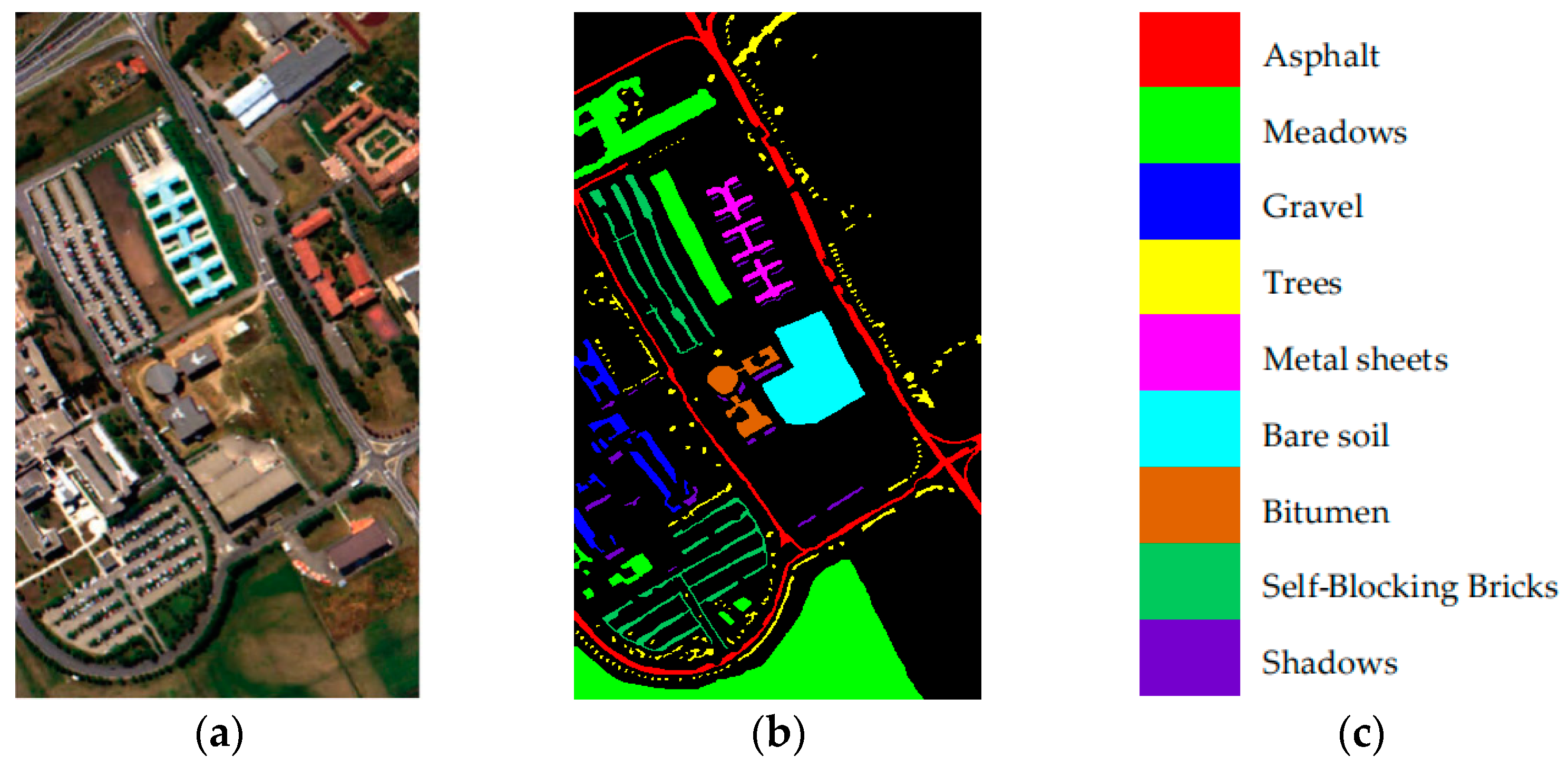
3.1. Data Description

A total of three publicly datasets (https://github.com/gokriznastic/HybridSN (accessed on 14 March 2022) were selected for the experiments to validate the classification performance of the proposed model, namely Indian Pines (IP), Pavia University (PU) and Salinas Valley (SV).
The IP data set consists of 145 × 145 pixels. It includes 220 contiguous spectral bands in the wavelength range of 400–2500 nm. The spatial resolution was 20 m. It was collected by a sensor in northwestern Indiana (AVIRIS). After removing 20 absorption bands, we selected the remaining 200 bands for study. The data were divided into 16 categories containing a variety of crops, such as corn, soybeans, etc. The samples were unevenly distributed, as detailed in Table 1. We randomly selected 10% of each category as the training set. The false-color image and ground-truth map correspond to (a) and (b) in Figure 5, respectively.
The PU dataset was obtained by spectral imager in the wavelength range of 430–860 nm and contains 115 bands in total. The spatial resolution was 1.3 m. It was collected by the Reflection Optical System Imaging Spectrometer (ROSIS). We removed 12 noisy bands and used the remaining 103 bands for the experiments. The dataset covered 610 × 340 pixels and contained 9 feature classes in total. Table 2 shows the details of the dataset. We used 5% of the data for training. The false-color image and ground-truth map correspond to (a) and (b) in Figure 6, respectively.
The Salinas dataset is an image of the SV taken by the VIRIS imaging spectrometer with a spatial resolution of 3.7 m, and collected by the Airborne Visible Infrared Imaging Spectrometer (AVIRIS) in Salinas Valley, California. The original dataset consists of 224 bands; we remove the water absorbing bands and the bands affected by noise and use the remaining 204 bands for the experiment. The dataset has a size of 512 × 217 and contains 16 categories, mainly various crops, such as broccoli green weeds, celery and Lettuce_romaine, etc. Table 3 shows the details of the dataset. We use 5% of the dataset for training. The false-color image and ground-truth map correspond to (a) and (b) in Figure 7, respectively.

3.2. Experimental Setting

A total of six classification evaluation metrics are used in this paper: OA, AA, Kappa, training time, testing time, and accuracy of each class. In addition, we offer visualization of the classification results. To ensure fairness, we conducted ten independent experiments on each dataset, and each experiment randomly selected 10% of the data on the IP dataset, 5% of the data on the PU and SV datasets as the training set, and the rest as the test set.
The proposed method was run in the PyTorch environment. All experiments in this paper were implemented on the same computer running on an NVIDIA GeForce RTX 3060 GPU and an 11th Gen Intel(R) Core(TM) i7-11700 CPU with 16 GB of RAM. The initial learning rate was set to le − 3, and the initial optimizer chosen was the Adam optimizer. The batch size of all three datasets was 64, and 100 training epochs were set for each dataset.

3.3. Classification Performance

We compared the method presented in this paper with several state-of-the-art HSI classification methods to evaluate its hyperspectral classification performance. These included CNN-based methods, namely 1-D CNN [33], 2-D CNN [57], 3-D CNN [35], 3D-2D hybrid CNN method HybridSN [40], the double-branch dual-attention mechanism method DBDA [47], and the transformer-based method SSFTT [54]. For the sake of fairness, we used uniform settings for all methods and conducted experiments on each of the three datasets. We took the best results from ten experiments for presentation, where the best results in each row are bolded.
On the IP dataset, the 1-D CNN method had the shortest training and testing times. Since only spectral information was used for classification, the accuracy was low. The 2-D CNN method using spatial information for classification further improved the results compared to the 1-D CNN method. In 3-D CNNs, spatial and spectral information were used jointly to further improve classification accuracy, but this took more time. HybridSN combines 3D and 2D to reduce the time cost while improving the classification accuracy. DBDA introduced the attention mechanism for classification. SSFTT combined Transformer with CNN and achieved good classification results. The classification accuracy of our method was approximately 1.2% higher than SSFTT and outperformed other methods in eleven categories, six of which had no incorrect pixels. The results of the comparison experiments on the IP dataset are shown in Table 4. To compare the classification results more visually, Figure 8 shows the ground-truth map and the classification result plots for the seven experiments. It can be observed that the 1-D CNN had a large amount of noise in the visual images and the classification accuracy was low, followed by the 2-D CNN with relatively poor classification results. The 3-D CNN, HybridSN, DBDA and SSFTT had relatively smooth visual images. Compared with other methods, the classification map produced by our method was closest to the ground-truth map, and the edges of the features were clearer.
Table 5 shows the results of the PU dataset comparison experiments. Our proposed method achieved higher accuracy on OA, AA and Kappa than any other method. We achieved higher accuracy in six categories, three of which reached 100% accuracy. Figure 9a–h show the classification maps of the ground-truth map, 1-D CNN, 2-D CNN, 3-D CNN, HybridSN, DBDA, SSFTT and our method, respectively. The classification maps of our method are closest to the ground-truth map, in which the blue lake region (category 6) is easily mixed with green pixels by the other methods; our method could better identify the category in this region. In addition, it verified the accuracy of our method’s classification.
The results of the comparison experiments on the SV dataset are shown in Table 6. Our proposed method achieved higher accuracy on OA, AA and Kappa than any other methods. We achieved the best accuracy in twelve categories. To compare the classification results more intuitively, Figure 10 shows the false-color image, ground-truth map and the classification result images of the seven experiments. We can conclude from comparing the border regions in the image that our method produces the best delineation of the boundaries, thus validating the effectiveness of our method’s classification.
A comparison of training and testing times of all methods tested for the three datasets is shown in Table 7. 3-D CNN requires longer for both training and testing. Our method uses 3-D CNNs to extract spatial–spectral information, which inevitably increases the time. On the IP dataset, the training time of DBAA-CNN were faster than the other methods besides 1-D CNN. The reduction in time spent by our method is also significant on the PU and SV datasets. In particular, our method’s training time on the SV dataset was shorter than that of the other compared methods, which further indicates that our method improves classification accuracy and efficiency while reducing time.

3.4. Parameter Analysis

HSI classification is to determine the class of the central pixel of the cut block. The larger the cut block is, the more neighboring pixels it contains, which may help to classify the central pixel, but also inevitably causes an increase in computational cost. Thus, we analyzed the size of the window on three datasets. Table 8 and Figure 11 show the impact of the window size of the input data on the classification results. We can observe from the table that as the window size increases, the complexity of the computation increases and the training time increases, too. Moreover, the average accuracy rises and then falls as the window size increases. Considering the two factors of computational volume and classification accuracy, the window size used for three datasets was 13 × 13.
We also chose a different number of bands to test the effects on the classification performance. In HSI classification, the number of bands determines how much spectral information is used by the network. The fewer the bands, the less spectral information is used and the shorter the time spent, and vice versa. The effect of the number of bands on the classification performance is shown in Figure 12. It can be observed that OA increases with the number of bands. In summary, the number of bands for three datasets was chosen to be 80, considering stability and generalization.

3.5. Ablation Experiments

We evaluate the efficacy of each module in a comprehensive manner by conducting ablation experiments on the IP dataset. Table 9 displays the experimental results for different module settings. The study of the ablation experiment data indicates that the three modules cooperate to produce better classification outcomes, further demonstrating the efficacy of our suggested paradigm.

4. Discussion

Based on the experimental results, the DBAA-CNN performs significantly better than other classification methods. The 1-D CNN has the worst classification results on the three datasets because the method loses spatial information due to its one-dimensional input data. The 2-D CNN method takes into account the spatial information; thus, the OA was improved compared with the 1-D CNN method. The 3-D CNN method extracts the features directly from the 3D data, which better preserves the original features of the data. The HybridSN and DBDA methods combine 2-D and 3-D CNN to extract spatial and spectral features, integrate them and feed them into the classifier. The SSFTT approach adds the transformer to extract spectral features. The DBDA approach adds the channel and spectral attention blocks to improve the classification effect but it consumed more time on the PU and SV datasets. Our method had the best classification results on the three datasets. The DBAA-CNN combines advantages of the attention mechanism and also reduces time consumption, which reduces the training and testing time while improving the classification results.
Additionally, the performance of classification was evaluated with different window sizes and the amount of bands. The final window size of 13 × 13 was chosen by considering the OA and testing time. In order to retain more spectral information, we chose a different number of bands for the experiments, OA increases with the number of bands, but more bands inevitably contain redundant information, which causes the OA to rise and then fall, so the number of bands is finally chosen to be 80. Table 8 shows that our method’s training and testing times on the three datasets are advantageous, which indicates that we have improved the efficiency of classification.
As shown in Table 8, the training and testing times of our method on three datasets is advantageous, which indicates that we have improved the efficiency of classification.

5. Conclusions

We presented a novel DBAA-CNN classification method for HSI in this paper. A spatial–spectral branch and a spectral attention branch make up the method. The spatial-spectral branch combines 3-D CNN with multiscale squeeze-and-excitation pyramid attention. 3-D convolutional layers are used to obtain shallow spatial–spectral features. The multiscale pyramid module is used to further mine the multiscale information of HSI, and then, integrate the multiscale spatial information with cross-channel attention. The spectral attention branch maps original features to the spectral interaction space for feature representation and learning. In order to generate spatial–spectral features for classification, the features of two branches are finally combined. This enhances the ability of the feature map to extract valid information by utilizing the attention mechanism. Experiments and analysis of the three datasets demonstrate that the method effectively enhances classification performance and reduces time consumption. In future work, we will consider combining graph convolution networks (GCN) to jointly extract spatial and spectral features, thus further enhancing the efficiency and accuracy of classification.

Author Contributions

Conceptualization, M.J.; Methodology, W.H.; Validation, Z.Z.; Supervision, L.S. All authors have read and agreed to the published version of the manuscript.

Funding

This research was funded by Scientific and technological key project in Henan Province, grant number 212102210102 and 212102210105.

Data Availability Statement

The data presented in this study are available in article.

Acknowledgments

The authors would like to thank the editors and reviewers for their advice.

Conflicts of Interest

The authors declare no conflict of interest.

Abbreviations

The following abbreviations are used in this manuscript:
CNNConvolutional Neural Network
HSIHyperspectral Image
PSAPyramid Squeeze-And-Excitation Attention
KNNK-Nearest Neighbor
SVMSupport Vector Machines
SAEStacked Auto Encoder
DBNDeep Belief Networks
RNNRecurrent Neural Networks
NLPNatural Language Processing
SESqueeze-and-Excitation
GAPGlobal Average Pooling
FCFully Connected
SACSqueeze And Concat
IPIndian Pines
PUPavia University
SVSalinas Valley
OAOverall Accuracy
AAAverage Accuracy
KappaKappa Coefficient

References

  1. Huang, W.; Li, G.; Chen, Q.; Ju, M.; Qu, J. CF2PN: A Cross-Scale Feature Fusion Pyramid Network Based Remote Sensing Target Detection. Remote Sens. 2021, 13, 847. [Google Scholar] [CrossRef]
  2. Huang, W.; Li, G.; Jin, B.; Chen, Q.; Yin, J.; Huang, L. Scenario Context-Aware-Based Bidirectional Feature Pyramid Network for Remote Sensing Target Detection. IEEE Geosci. Remote Sens. Lett. 2022, 19, 1–5. [Google Scholar] [CrossRef]
  3. Sabbah, S.; Rusch, P.; Eichmann, J.; Gerhard, J.-H.; Harig, R. Remote Sensing of Gases by Hyperspectral Imaging: Results of Field Measurements. In Proceedings of the Electro-Optical Remote Sensing, Photonic Technologies, and Applications VI, Edinburgh, UK, 24–27 September 2012; Kamerman, G.W., Steinvall, O., Lewis, K.L., Hollins, R.C., Merlet, T.J., Gruneisen, M.T., Dusek, M., Rarity, J.G., Bishop, G.J., Gonglewski, J., Eds.; SPIE: Bellingham, WA, USA, 2012; Volume 8542, p. 854227. [Google Scholar]
  4. Gevaert, C.M.; Suomalainen, J.; Tang, J.; Kooistra, L. Generation of Spectral–Temporal Response Surfaces by Combining Multispectral Satellite and Hyperspectral UAV Imagery for Precision Agriculture Applications. IEEE J. Sel. Top. Appl. Earth Obs. Remote Sens. 2015, 8, 3140–3146. [Google Scholar] [CrossRef]
  5. Shimoni, M.; Haelterman, R.; Perneel, C. Hypersectral Imaging for Military and Security Applications: Combining Myriad Processing and Sensing Techniques. IEEE Geosci. Remote Sens. Mag. 2019, 7, 101–117. [Google Scholar] [CrossRef]
  6. Ardouin, J.-P.; Levesque, J.; Rea, T.A. A Demonstration of Hyperspectral Image Exploitation for Military Applications. In Proceedings of the 2007 10th International Conference on Information Fusion, Quebec, QC, Canada, 9–12 July 2007; pp. 1–8. [Google Scholar]
  7. Fan, J.; Zhou, N.; Peng, J.; Gao, L. Hierarchical Learning of Tree Classifiers for Large-Scale Plant Species Identification. IEEE Trans. Image Process. 2015, 24, 4172–4184. [Google Scholar] [PubMed]
  8. Hsieh, T.-H.; Kiang, J.-F. Comparison of CNN Algorithms on Hyperspectral Image Classification in Agricultural Lands. Sensors 2020, 20, 1734. [Google Scholar] [CrossRef] [PubMed] [Green Version]
  9. Li, S.; Song, W.; Fang, L.; Chen, Y.; Ghamisi, P.; Benediktsson, J.A. Deep Learning for Hyperspectral Image Classification: An Overview. IEEE Trans. Geosci. Remote Sens. 2019, 57, 6690–6709. [Google Scholar] [CrossRef] [Green Version]
  10. Dong, Y.; Liang, T.; Zhang, Y.; Du, B. Spectral–Spatial Weighted Kernel Manifold Embedded Distribution Alignment for Remote Sensing Image Classification. IEEE Trans. Cybern. 2021, 51, 3185–3197. [Google Scholar] [CrossRef]
  11. Yue, J.; Fang, L.; Rahmani, H.; Ghamisi, P. Self-Supervised Learning With Adaptive Distillation for Hyperspectral Image Classification. IEEE Trans. Geosci. Remote Sens. 2022, 60, 1–13. [Google Scholar] [CrossRef]
  12. Cheng, G.; Li, Z.; Han, J.; Yao, X.; Guo, L. Exploring Hierarchical Convolutional Features for Hyperspectral Image Classification. IEEE Trans. Geosci. Remote Sens. 2018, 56, 6712–6722. [Google Scholar] [CrossRef]
  13. Bioucas-Dias, J.M.; Plaza, A.; Camps-Valls, G.; Scheunders, P.; Nasrabadi, N.; Chanussot, J. Hyperspectral Remote Sensing Data Analysis and Future Challenges. IEEE Geosci. Remote Sens. Mag. 2013, 1, 6–36. [Google Scholar] [CrossRef] [Green Version]
  14. Awad, M.M. Cooperative Evolutionary Classification Algorithm for Hyperspectral Images. J. Appl. Remote Sens. 2020, 14, 016509. [Google Scholar] [CrossRef]
  15. Li, J.; Khodadadzadeh, M.; Plaza, A.; Jia, X.; Bioucas-Dias, J.M. A Discontinuity Preserving Relaxation Scheme for Spectral–Spatial Hyperspectral Image Classification. IEEE J. Sel. Top. Appl. Earth Obs. Remote Sens. 2016, 9, 625–639. [Google Scholar] [CrossRef]
  16. Wambugu, N.; Chen, Y.; Xiao, Z.; Tan, K.; Wei, M.; Liu, X.; Li, J. Hyperspectral Image Classification on Insufficient-Sample and Feature Learning Using Deep Neural Networks: A Review. Int. J. Appl. Earth Obs. Geoinf. 2021, 105, 102603. [Google Scholar] [CrossRef]
  17. Fabiyi, S.D.; Murray, P.; Zabalza, J.; Ren, J. Folded LDA: Extending the Linear Discriminant Analysis Algorithm for Feature Extraction and Data Reduction in Hyperspectral Remote Sensing. IEEE J. Sel. Top. Appl. Earth Obs. Remote Sens. 2021, 14, 12312–12331. [Google Scholar] [CrossRef]
  18. Duan, Y.; Huang, H.; Tang, Y. Local Constraint-Based Sparse Manifold Hypergraph Learning for Dimensionality Reduction of Hyperspectral Image. IEEE Trans. Geosci. Remote Sens. 2021, 59, 613–628. [Google Scholar] [CrossRef]
  19. Luo, F.; Zhang, L.; Zhou, X.; Guo, T.; Cheng, Y.; Yin, T. Sparse-Adaptive Hypergraph Discriminant Analysis for Hyperspectral Image Classification. IEEE Geosci. Remote Sens. Lett. 2020, 17, 1082–1086. [Google Scholar] [CrossRef]
  20. Duan, Y.; Huang, H.; Li, Z.; Tang, Y. Local Manifold-Based Sparse Discriminant Learning for Feature Extraction of Hyperspectral Image. IEEE Trans. Cybern. 2021, 51, 4021–4034. [Google Scholar] [CrossRef]
  21. Ma, L.; Crawford, M.M.; Tian, J. Local Manifold Learning-Based $k$ -Nearest-Neighbor for Hyperspectral Image Classification. IEEE Trans. Geosci. Remote Sens. 2010, 48, 4099–4109. [Google Scholar] [CrossRef]
  22. Fauvel, M.; Benediktsson, J.A.; Chanussot, J.; Sveinsson, J.R. Spectral and Spatial Classification of Hyperspectral Data Using SVMs and Morphological Profiles. IEEE Trans. Geosci. Remote Sens. 2008, 46, 3804–3814. [Google Scholar] [CrossRef]
  23. Melgani, F.; Bruzzone, L. Classification of Hyperspectral Remote Sensing Images with Support Vector Machines. IEEE Trans. Geosci. Remote Sens. 2004, 42, 1778–1790. [Google Scholar] [CrossRef] [Green Version]
  24. Huang, W.; Huang, Y.; Wang, H.; Liu, Y.; Shim, H.J. Local Binary Patterns and Superpixel-Based Multiple Kernels for Hyperspectral Image Classification. IEEE J. Sel. Top. Appl. Earth Obs. Remote Sens. 2020, 13, 4550–4563. [Google Scholar] [CrossRef]
  25. Paoletti, M.E.; Haut, J.M.; Pereira, N.S.; Plaza, J.; Plaza, A. Ghostnet for Hyperspectral Image Classification. IEEE Trans. Geosci. Remote Sens. 2021, 59, 10378–10393. [Google Scholar] [CrossRef]
  26. LeCun, Y.; Bengio, Y.; Hinton, G. Deep Learning. Nature 2015, 521, 436–444. [Google Scholar] [CrossRef]
  27. Zhang, K.; Zuo, W.; Zhang, L. FFDNet: Toward a Fast and Flexible Solution for CNN-Based Image Denoising. IEEE Trans. Image Process. 2018, 27, 4608–4622. [Google Scholar] [CrossRef] [Green Version]
  28. Remote Sensing|Free Full-Text|Combing Triple-Part Features of Convolutional Neural Networks for Scene Classification in Remote Sensing. Available online: https://www.mdpi.com/2072-4292/11/14/1687 (accessed on 12 July 2022).
  29. Chen, Y.; Lin, Z.; Zhao, X.; Wang, G.; Gu, Y. Deep Learning-Based Classification of Hyperspectral Data. IEEE J. Sel. Top. Appl. Earth Obs. Remote Sens. 2014, 7, 2094–2107. [Google Scholar] [CrossRef]
  30. Chen, Y.; Zhao, X.; Jia, X. Spectral–Spatial Classification of Hyperspectral Data Based on Deep Belief Network. IEEE J. Sel. Top. Appl. Earth Obs. Remote Sens. 2015, 8, 2381–2392. [Google Scholar] [CrossRef]
  31. Mou, L.; Ghamisi, P.; Zhu, X.X. Deep Recurrent Neural Networks for Hyperspectral Image Classification. IEEE Trans. Geosci. Remote Sens. 2017, 55, 3639–3655. [Google Scholar] [CrossRef] [Green Version]
  32. Hang, R.; Li, Z.; Ghamisi, P.; Hong, D.; Xia, G.; Liu, Q. Classification of Hyperspectral and LiDAR Data Using Coupled CNNs. IEEE Trans. Geosci. Remote Sens. 2020, 58, 4939–4950. [Google Scholar] [CrossRef] [Green Version]
  33. Hu, W.; Huang, Y.; Wei, L.; Zhang, F.; Li, H. Deep Convolutional Neural Networks for Hyperspectral Image Classification. J. Sens. 2015, 2015, 258619. [Google Scholar] [CrossRef]
  34. Makantasis, K.; Karantzalos, K.; Doulamis, A.; Doulamis, N. Deep Supervised Learning for Hyperspectral Data Classification through Convolutional Neural Networks. In Proceedings of the 2015 IEEE International Geoscience and Remote Sensing Symposium (IGARSS), Milan, Italy, 26–31 July 2015; pp. 4959–4962. [Google Scholar]
  35. Chen, Y.; Jiang, H.; Li, C.; Jia, X.; Ghamisi, P. Deep Feature Extraction and Classification of Hyperspectral Images Based on Convolutional Neural Networks. IEEE Trans. Geosci. Remote Sens. 2016, 54, 6232–6251. [Google Scholar] [CrossRef] [Green Version]
  36. Ben Hamida, A.; Benoit, A.; Lambert, P.; Ben Amar, C. 3-D Deep Learning Approach for Remote Sensing Image Classification. IEEE Trans. Geosci. Remote Sens. 2018, 56, 4420–4434. [Google Scholar] [CrossRef] [Green Version]
  37. Li, Y.; Zhang, H.; Shen, Q. Spectral-Spatial Classification of Hyperspectral Imagery with 3D Convolutional Neural Network. Remote Sens. 2017, 9, 67. [Google Scholar] [CrossRef] [Green Version]
  38. Zhong, Z.; Li, J.; Luo, Z.; Chapman, M. Spectral–Spatial Residual Network for Hyperspectral Image Classification: A 3-D Deep Learning Framework. IEEE Trans. Geosci. Remote Sens. 2018, 56, 847–858. [Google Scholar] [CrossRef]
  39. Paoletti, M.E.; Haut, J.M.; Fernandez-Beltran, R.; Plaza, J.; Plaza, A.J.; Pla, F. Deep Pyramidal Residual Networks for Spectral–Spatial Hyperspectral Image Classification. IEEE Trans. Geosci. Remote Sens. 2019, 57, 740–754. [Google Scholar] [CrossRef]
  40. Roy, S.K.; Krishna, G.; Dubey, S.R.; Chaudhuri, B.B. HybridSN: Exploring 3-D–2-D CNN Feature Hierarchy for Hyperspectral Image Classification. IEEE Geosci. Remote Sens. Lett. 2020, 17, 277–281. [Google Scholar] [CrossRef] [Green Version]
  41. Xu, X.; Li, W.; Ran, Q.; Du, Q.; Gao, L.; Zhang, B. Multisource Remote Sensing Data Classification Based on Convolutional Neural Network. IEEE Trans. Geosci. Remote Sens. 2018, 56, 937–949. [Google Scholar] [CrossRef]
  42. Wang, F.; Jiang, M.; Qian, C.; Yang, S.; Li, C.; Zhang, H.; Wang, X.; Tang, X. Residual Attention Network for Image Classification. In Proceedings of the IEEE Conference on Computer Vision and Pattern Recognition (CVPR), Honolulu, HI, USA, 21–26 July 2017; pp. 3156–3164. [Google Scholar]
  43. Woo, S.; Park, J.; Lee, J.-Y.; Kweon, I.S. CBAM: Convolutional Block Attention Module. In Proceedings of the Computer Vision (ECCV), Munich, Germany, 8–14 September 2018; Ferrari, V., Hebert, M., Sminchisescu, C., Weiss, Y., Eds.; Springer International Publishing Ag: Cham, Switzerland, 2018; Volume 11211, pp. 3–19. [Google Scholar]
  44. Hu, J.; Shen, L.; Albanie, S.; Sun, G.; Wu, E. Squeeze-and-Excitation Networks. IEEE Trans. Pattern Anal. Mach. Intell. 2020, 42, 2011–2023. [Google Scholar] [CrossRef] [PubMed] [Green Version]
  45. Haut, J.M.; Paoletti, M.E.; Plaza, J.; Plaza, A.; Li, J. Visual Attention-Driven Hyperspectral Image Classification. IEEE Trans. Geosci. Remote Sens. 2019, 57, 8065–8080. [Google Scholar] [CrossRef]
  46. Sun, H.; Zheng, X.; Lu, X.; Wu, S. Spectral–Spatial Attention Network for Hyperspectral Image Classification. IEEE Trans. Geosci. Remote Sens. 2020, 58, 3232–3245. [Google Scholar] [CrossRef]
  47. Li, R.; Zheng, S.; Duan, C.; Yang, Y.; Wang, X. Classification of Hyperspectral Image Based on Double-Branch Dual-Attention Mechanism Network. Remote Sens. 2020, 12, 582. [Google Scholar] [CrossRef] [Green Version]
  48. Vaswani, A.; Shazeer, N.; Parmar, N.; Uszkoreit, J.; Jones, L.; Gomez, A.N.; Kaiser, Ł.; Polosukhin, I. Attention Is All You Need. In Advances in Neural Information Processing Systems; Curran Associates, Inc.: Red Hook, NY, USA, 2017; Volume 30. [Google Scholar]
  49. Raffel, C.; Shazeer, N.; Roberts, A.; Lee, K.; Narang, S.; Matena, M.; Zhou, Y.; Li, W.; Liu, P.J. Exploring the Limits of Transfer Learning with a Unified Text-to-Text Transformer. J. Mach. Learn. Res. 2020, 21, 1–67. [Google Scholar]
  50. Dosovitskiy, A.; Beyer, L.; Kolesnikov, A.; Weissenborn, D.; Zhai, X.; Unterthiner, T.; Dehghani, M.; Minderer, M.; Heigold, G.; Gelly, S.; et al. An Image Is Worth 16×16 Words: Transformers for Image Recognition at Scale. arXiv 2021, arXiv:2010.11929. [Google Scholar]
  51. Hu, X.; Li, T.; Zhou, T.; Liu, Y.; Peng, Y. Contrastive Learning Based on Transformer for Hyperspectral Image Classification. Appl. Sci. 2021, 11, 8670. [Google Scholar] [CrossRef]
  52. Remote Sensing|Free Full-Text|Improved Transformer Net for Hyperspectral Image Classification. Available online: https://www.mdpi.com/2072-4292/13/11/2216 (accessed on 1 September 2022).
  53. Hong, D.; Han, Z.; Yao, J.; Gao, L.; Zhang, B.; Plaza, A.; Chanussot, J. SpectralFormer: Rethinking Hyperspectral Image Classification With Transformers. IEEE Trans. Geosci. Remote Sens. 2022, 60, 1–15. [Google Scholar] [CrossRef]
  54. Sun, L.; Zhao, G.; Zheng, Y.; Wu, Z. Spectral–Spatial Feature Tokenization Transformer for Hyperspectral Image Classification. IEEE Trans. Geosci. Remote Sens. 2022, 60, 1–14. [Google Scholar]
  55. Licciardi, G.; Marpu, P.R.; Chanussot, J.; Benediktsson, J.A. Linear Versus Nonlinear PCA for the Classification of Hyperspectral Data Based on the Extended Morphological Profiles. IEEE Geosci. Remote Sens. Lett. 2012, 9, 447–451. [Google Scholar] [CrossRef] [Green Version]
  56. Zhang, H.; Zu, K.; Lu, J.; Zou, Y.; Meng, D. EPSANet: An Efficient Pyramid Squeeze Attention Block on Convolutional Neural Network. In Proceedings of the Asian Conference on Computer Vision (ACCV), Macau SAR, China, 4–8 December 2022. [Google Scholar]
  57. Zhao, W.; Du, S. Spectral–Spatial Feature Extraction for Hyperspectral Image Classification: A Dimension Reduction and Deep Learning Approach. IEEE Trans. Geosci. Remote Sens. 2016, 54, 4544–4554. [Google Scholar] [CrossRef]
Figure 1. The structure of 3-D convolution.
Remotesensing 14 06158 g001
Figure 2. SE block.
Figure 2. SE block.
Remotesensing 14 06158 g002
Figure 3. Framework of the DBAA-CNN for HSI classification.
Remotesensing 14 06158 g003
Figure 4. Detailed description of the proposed PSA module when g = 4.
Remotesensing 14 06158 g004
Figure 5. IP dataset. (a) False-color image. (b) Ground-truth map. (c) Color coding for each category.
Remotesensing 14 06158 g005
Figure 6. PU dataset. (a) False-color image. (b) Ground-truth map. (c) Color coding for each category.
Remotesensing 14 06158 g006
Figure 7. SV dataset. (a) False-color image. (b) Ground-truth map. (c) Color coding for each category.
Remotesensing 14 06158 g007
Figure 8. Classification maps of the IP dataset. (a) Ground-truth map. (b) 1-D CNN. (c) 2-D CNN. (d) 3-D CNN. (e) HybridSN. (f) DBDA. (g) SSFTT. (h) Ours.
Remotesensing 14 06158 g008
Figure 9. Classification maps of PU dataset. (a) Ground-truth map. (b) 1-D CNN. (c) 2-D CNN. (d) 3-D CNN. (e) HybridSN. (f) DBDA. (g) SSFTT. (h) Ours.
Remotesensing 14 06158 g009
Figure 10. Classification maps of SV. (a) Ground-truth map. (b) 1-D CNN. (c) 2-D CNN. (d) 3-D CNN. (e) HybridSN. (f) DBDA. (g) SSFTT. (h) Ours.
Remotesensing 14 06158 g010
Figure 11. The effect of different window sizes on the OA of DBAA-CNN.
Remotesensing 14 06158 g011
Figure 12. The effect of different numbers of bands on the OA of DBAA-CNN.
Remotesensing 14 06158 g012
Table 1. Training and test sample division of each class in the IP dataset.
NO.ClassTrainTest
1Alfalfa541
2Corn—notill1431285
3Corn—mintill83747
4Corn24213
5Grass–pasture48435
6Grass-tree73657
7Grass–pasture–mowed325
8Hay—windrowed48430
9Oats218
10Soybeans—notill97875
11Soybeans—mintill2452210
12Soybeans—clean59534
13Wheat20185
14Woods1261139
15Buildings–grass–trees39347
16Stone–steel–towers984
Total10249225
Table 2. Training and test sample division of each class in the PU dataset.
NO.ClassTrainTest
1Asphalt3326299
2Meadows93217,717
3Gravel1051994
4Trees1532911
5Metal sheets671278
6Bare soil2514778
7Bitumen671263
8Self-Blocking bricks1843498
9Shadows47900
Total213840,638
Table 3. Training and test sample division of each class in the SV dataset.
NO.ClassTrainTest
1Broccoli green weeds_11001909
2Broccoli green weeds_21863540
3Fallow991877
4Fallow_rough_plow701324
5Fallow_smooth1342544
6Stubble1983761
7Celery1793400
8Grapes_untrained56410,707
9Soil_vinyard_develop3105893
10Corn_senesced_green_weeds1643114
11Lettuce_romaine_4wk531015
12Lettuce_romaine_5wk961831
13Lettuce_romaine_6wk46870
14Lettuce_romaine_7wk541016
15Vinyard_untrained3646904
16Vinyard_vertical_trellis901717
Total270751,422
Table 4. Classification results by different methods for the IP dataset (optimal results are bolded).
Class No.1-D CNN2-D CNN3-D CNNHybridSNDBDASSFTTOurs
126.8385.3748.7868.2997.5697.56100
271.7588.4892.1499.8489.9694.2496.73
353.6879.9298.5395.7296.7997.0599.06
452.1176.0687.7992.4999.0697.65100
586.9090.3498.3994.7199.5499.0897.93
694.0698.4896.3510097.1198.3299.85
744.0084.0010060.0092.0088.00100
898.8497.9110010099.77100100
933.3383.3372.2210010072.22100
1066.4091.8996.8096.0097.0396.9198.74
1181.4494.2196.3898.6998.6498.7399.64
1276.4085.9694.1996.0796.6398.3196.25
1398.3899.4698.3810096.2297.2899.46
1495.5295.4399.3998.9595.87100100
1563.9879.5491.0796.5497.9897.1199.42
1679.7688.1080.9544.0589.2989.1698.80
OA(%)78.3890.1095.7597.2796.4997.6998.89
AA(%)70.2188.6590.7190.0896.4795.1099.12
Kappa × 10075.1789.7095.1896.8895.3997.3698.74
Table 5. Classification results by different methods for the PU dataset (optimal results are bolded).
Class No.1-D CNN2-D CNN3-D CNNHybridSNDBDASSFTTOurs
194.2295.2287.9398.8497.9899.1399.17
297.1796.6599.7799.9898.7899.6099.92
382.5587.6696.7498.9998.4598.4096.58
493.8298.9798.2898.9796.7498.2199.66
510099.7710099.37100100100
690.7992.9796.4010098.3599.98100
786.7088.9295.0999.9297.47100100
882.9179.2594.3796.1196.3198.4898.83
910099.8999.6797.1110096.5699.78
OA(%)93.6194.1596.6899.2798.2599.2799.54
AA(%)92.0293.2696.4798.8198.2398.9399.33
Kappa × 10091.5392.2895.5999.0397.8999.0999.39
Table 6. Classification results by different methods for the SV dataset (optimal results are bolded).
Class No.CNN1DCNN2DCNN3DHybridSNDBDASSFTTOurs
199.7910010010099.9099.84100
299.9499.8910010099.7298.98100
399.7399.8410010099.6898.61100
499.7099.6298.9410098.9498.79100
594.5898.8299.8899.4999.9299.8099.88
699.0299.9210010098.7898.7099.89
799.9499.5999.9799.7098.7499.9199.47
887.8294.2399.9999.9310099.9399.96
999.8110010010099.54100100
1097.0598.7210010099.8799.58100
1196.6599.0110099.7099.80100100
1210010010010010097.76100
1398.9710010010099.8999.43100
1489.6799.2199.9010099.3199.6199.61
1577.8793.1496.4898.1998.6099.8399.46
1698.9599.6599.7110099.8399.3099.59
OA(%)93.6097.6499.4899.7199.5399.5599.85
AA(%)96.2298.8599.6899.7799.4999.3899.87
Kappa × 10092.8797.9999.4299.6799.5199.5099.83
Table 7. Training and testing time of all methods for the three datasets (optimal results are bolded).
MethodsIPPUSV
Train(s)Test(s)Train(s)Test(s)Train(s)Test(s)
1-D CNN39.730.36141.321.26187.381.64
2-D CNN64.770.86220.862.23207.111.87
3-D CNN126.961.36325.963.70296.716.52
HybridSN80.341.5875.592.5094.023.21
DBDA62.032.54196.7614.20215.2615.35
SSFTT57.131.90237.538.03300.3810.24
Ours52.191.20105.714.6488.055.32
Table 8. Performance impact of different window sizes.
Window SizesOATesting Time(s)
IPPUSVIPPUSV
9 × 998.3999.1999.420.663.013.76
11 × 1198.5299.4499.780.913.795.28
13 × 1398.8999.5499.851.204.645.32
15 × 1598.8999.4599.921.575.647.36
17 × 1798.5799.4799.951.686.3610.47
Table 9. Effect of different modules in the DBAA-CNN on the IP data set. (optimal results are bolded).
Cases3D ConvPSA ModuleSpectral Attention BranchOA (%)AA (%)Kappa (%)
1×96.4194.6695.90
2×95.7093.4295.38
3×97.9694.4295.10
498.8999.1298.74
The “×” in Table 9 indicates that the module is not included.
Publisher’s Note: MDPI stays neutral with regard to jurisdictional claims in published maps and institutional affiliations.

