Article

ArithFusion: An Arithmetic Deep Model for Temporal Remote Sensing Image Fusion

1
Department of Electrical & Computer Engineering, Old Dominion University, Norfolk, VA 23529, USA
2
Department of Computer Science, Old Dominion University, Norfolk, VA 23529, USA
3
Applied Research LLC, Rockville, MD 20850, USA
4
Maxar, Westminster, CO 80234, USA
*
Author to whom correspondence should be addressed.
Remote Sens. 2022, 14(23), 6160; https://doi.org/10.3390/rs14236160
Submission received: 31 October 2022 / Revised: 26 November 2022 / Accepted: 28 November 2022 / Published: 5 December 2022
(This article belongs to the Section Remote Sensing Image Processing)

Abstract

:
Different satellite images may consist of variable numbers of channels which have different resolutions, and each satellite has a unique revisit period. For example, the Landsat-8 satellite images have 30 m resolution in their multispectral channels, the Sentinel-2 satellite images have 10 m resolution in the pan-sharp channel, and the National Agriculture Imagery Program (NAIP) aerial images have 1 m resolution. In this study, we propose a simple yet effective arithmetic deep model for multimodal temporal remote sensing image fusion. The proposed model takes both low- and high-resolution remote sensing images at t 1 together with low-resolution images at a future time t 2 from the same location as inputs and fuses them to generate high-resolution images for the same location at t 2 . We propose an arithmetic operation applied to the low-resolution images at the two time points in feature space to take care of temporal changes. We evaluated the proposed model on three modality pairs for multimodal temporal image fusion, including downsampled WorldView-2/original WorldView-2, Landsat-8/Sentinel-2, and Sentinel-2/NAIP. Experimental results show that our model outperforms traditional algorithms and recent deep learning-based models by large margins in most scenarios, achieving sharp fused images while appropriately addressing temporal changes.

1. Introduction

Remote sensing imaging systems have become effective tools for vegetation monitoring [1,2,3,4], land cover detection [5], and human–nature interaction [6]. The availability of high temporal and spatial resolution remote sensed images plays a critical role in the success of these systems [7,8]. Obtaining high resolutions in both spatial and temporal domains by current satellite platforms remains difficult due to technical and budget limitations [9]. Different commercial remote sensing imagery providers produce different resolutions with various revisit frequencies and costs. For example, a single satellite usually has a low revisit frequency for the same area, and different satellites asynchronously sample the same area. WorldView-2 (WV-2) satellite and National Agriculture Imagery Program (NAIP) aerial images have very high spatial resolution but with very high prices (WV-2) and long revisit times (NAIP). Landsat and Sentinel-2 satellite images are free of charge and have medium spatial resolutions (10–60 m/pixel) [10].
One possible solution is to fuse multitemporal spatially coarse images with multi-temporal high-resolution images to achieve adequate resolutions in both temporal and spatial domains [11]. The fusion algorithm integrates high spatial, low temporal (HSLT) resolution images with low spatial, high temporal (LSHT) images. Through fusion, high-temporal-resolution images at medium spatial scale with a nominal revisit interval of few days can be achieved. Although significant advances have been achieved in recent years, the development of algorithms that can obtain sharp fused images and carry temporal changes in the image series remains a challenging task [12].
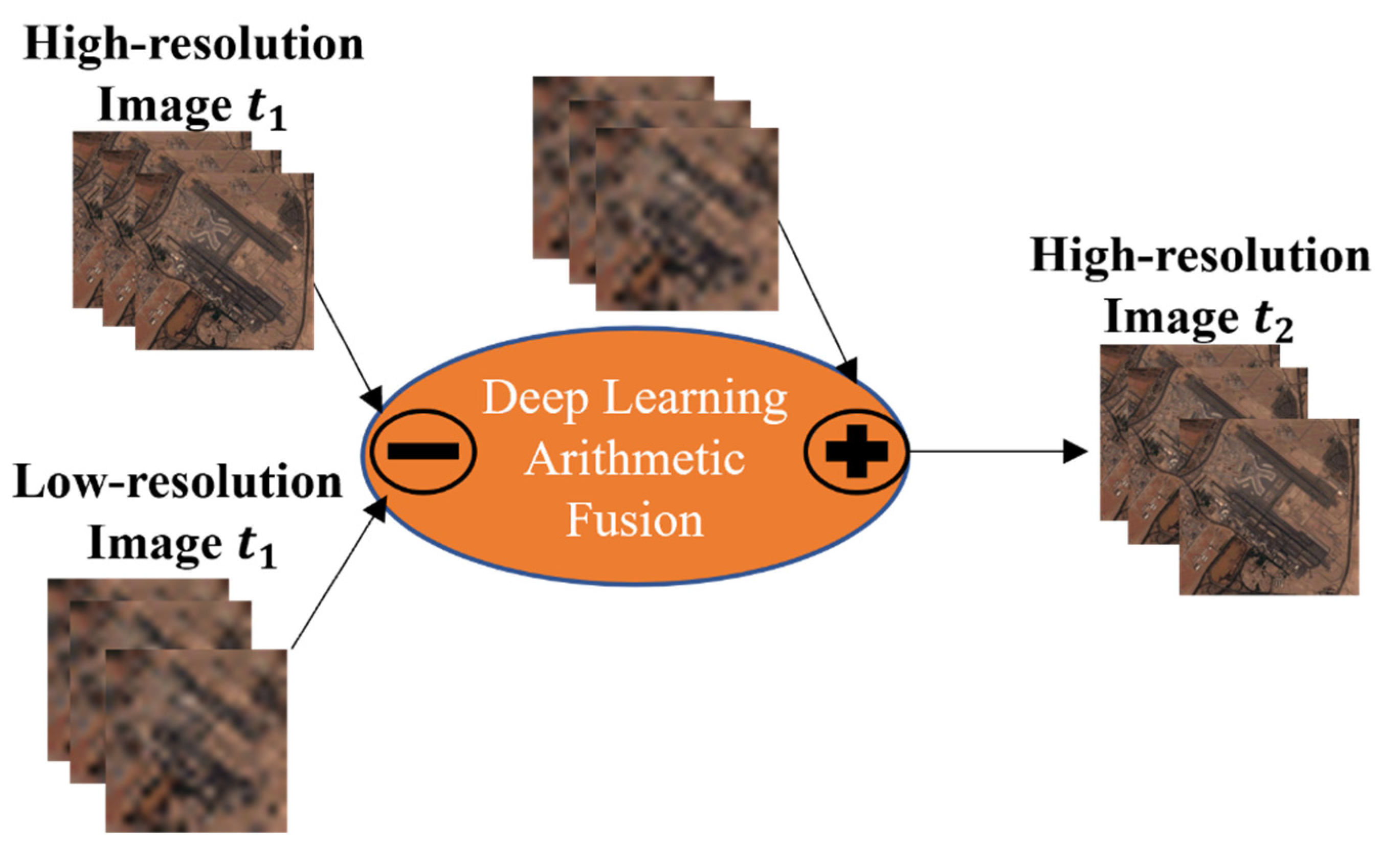
In this paper, we propose a deep learning model that takes full advantage of available temporal and spatial information using fusion to enhance spatial and temporal resolutions of remote sensing images, as shown in Figure 1. We propose an arithmetic fusion module to transform temporal changes in image series into high-resolution fused images. For the time stamps shown in Figure 1 from t 1 to t n , different resolution images from different systems may be available. Our ultimate goal is to produce a set of high-resolution images that can achieve a dense sampling of the Earth for continuous monitoring and change detection.
We focused only on RGB fusion in this paper for two reasons. First, there are applications where only high-resolution RGB images are available. Some images taken by aircraft/drones, such as the National Agriculture Imagery Program (NAIP) aerial images, are color images. Some high-resolution images such as Worldview only have RGB bands available for purchase. In addition, Google Maps uses RGB images from Maxar. The second reason is that some monitoring applications can be performed using RGB images only.
Our main contributions are:
  • We propose a deep learning model that performs arithmetic operations in feature space to fuse multimodal temporal remote sensing images. The arithmetic operation can effectively carry temporal changes and obtain high-resolution fused images, making it suitable for change detection applications.
  • We successfully applied the proposed model to fuse historical satellite image pairs, including Sentinel-2 satellite images (10 m spatial resolution), NAIP aerial images (1 m spatial resolution), Landsat-8 images (30 m spatial resolution), and Sentinel-2 images, to reconstruct high-resolution images. To the best of our knowledge, this is the first attempt to bridge the 10× resolution gap in remote sensing images.
  • We contribute a benchmark dataset that contains 45 pairs of low-resolution and high-resolution images collected by the LandSat-8 and Sentinel-2 satellites.
The paper is organized as follows. Section 2 reviews related work. Section 3 describes our proposed model. Section 4 introduces our experimental setups and datasets. Section 5 presents experimental results and discussions, and Section 6 concludes this paper.

2. Related Work

Traditional multi-temporal fusion algorithms for remote sensing images can be grouped into three categories:(1) filter-based, (2) unmixing-based, and (3) learning-based methods. In recent years, deep learning and geo-statistics have been shown to provide superb results.
In filter-based methods, image pixels in the fused image are calculated by selecting and weighting similar neighboring pixels from input images. The most popular classic spatial and temporal adaptive reflectance fusion model (STARFM) builds a simple approximating relationship between HSLT and LSHT pixels and searches similar neighboring pixels, based on spectral, temporal, and location distance to generate the fused image [13]. STARFM was improved by Zhu et al. [14] by assigning different coefficients for homogeneous and heterogeneous pixels. Shen et al. [15] performed further development by considering sensor observation differences. Filter-based methods require paired fine and coarse images from same day for training, which is not always possible in practice.
Zurita-Milla et al. [16] introduced an unmixing-based fusion method where the synthetic images are generated using the spatial information of Landsat/TM data and the spectral information of medium-resolution imaging spectrometer (MERIS) data. This method was later improved by the same research group [17]. The unmixing-based methods outperformed filter-based methods. However, the methods assume that there are no significant changes between the images to be fused, which is unrealistic in most cases.
Learning-based methods such as sparse representation learning were proposed in recent years [18,19], where a dictionary was first learned from different image modalities and a fused image was then generated by selecting and weighting elements in the learned dictionary. In those algorithms, feature extraction, dictionary learning, sparse coding, and image reconstruction were carried out separately, which ultimately increased the complexity of the algorithms. In addition, changes between different images were not well addressed.
Recently, area-to-point regression Kriging (ATPRK) based on geo-statistics was first introduced by Wang et al. for image fusion [20]. Later on, they applied ATPRK to fuse Landsat-8 Operational Land Imager (OLI) and Sentinel-2 Multispectral Imager (MSI) data and achieved better performances than STARFM [21], and it can address temporal changes. However, ATPRK is computationally expensive, and fused images are usually not sharp.
In the past few years, deep learning has made numerous contributions in computer vision [22], natural language processing [23,24], speech recognition [25,26], and remote sensing [27,28]. For example, Dong et al. developed a convolutional neural network (CNN) for image super-resolution [29]. Motivated by the CNN model, Song et al. [30] applied CNN to fuse MODIS and Landsat images. Li et al. improved the model by introducing the sensor bias-driven fusion method [31]. Shao et al. developed an extended super-resolution CNN (ESRCNN) model to blend Landsat-8 OLI and Sentinel-2 MSI data [12]. Chen et al. proposed a generative adversarial network (GAN) for feature level image fusion for Landsat/Sentinel-2 images [32] during their overlapping period. Their model achieved better results than those by non-deep learning methods. Zhang et al. developed a GAN-based remote sensing image spatio-temporal fusion method (STFGAN) using a feature-level fusion strategy to fuse Landsat and MODIS images. The model consisted of a two-stage end-to-end GAN framework. In the first stage, it enhanced the resolution of MODIS images and then fused features from MODIS and Landsat images to generate high resolution images.
Although deep learning-based models achieved excellent resolution enhancement in image fusion, handling temporal changes in image series remains a challenging task for most of the deep models. In change detection or monitoring applications, those changes are the most important attributes to focus on. While the ATPRK model can account for temporal changes, the model’s fusion results usually have inferior resolutions than those produced by deep models. In this paper, we propose a simple yet effective arithmetic fusion approach that can not only achieve resolution enhancement but also captures temporal changes. We evaluated our fusion models on four datasets, including Landsat-8, Sentinel-2, NAIP, and WV-2, for fusion. Experimental results show that temporal changes in these datasets can be accurately captured by our proposed model in the fused high-resolution images, potentially facilitating subsequent change detection tasks.

3. Methodology

3.1. Proposed Model

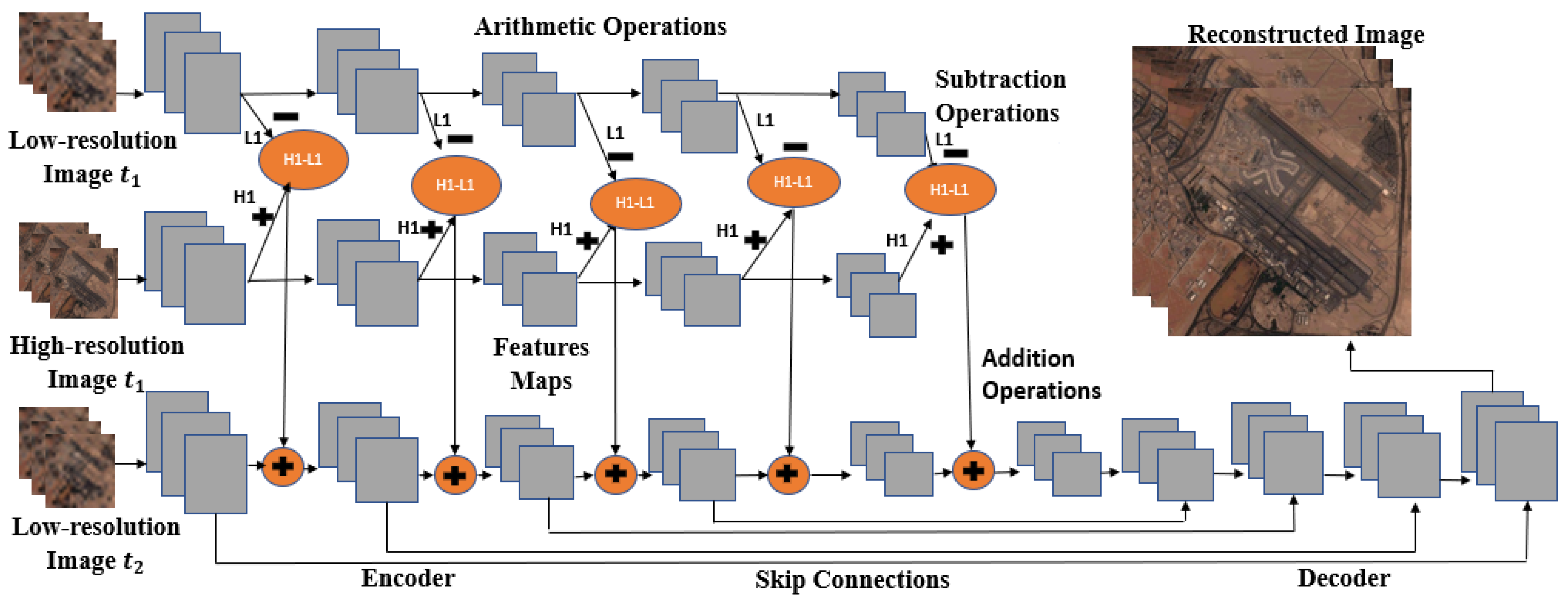
Figure 2 shows the diagram of the proposed approach. We feed low- and high-resolution images collected at t 1 and low-resolution images at t 2 as inputs. We then perform arithmetic operations to approximate a high-resolution image at t 2 . Mathematically, the fusion is described in Equation (1) as follows:
H t 2 = F   ( ( H t 1 L t 1 ) + L t 2 )  
where F(…) is the deep network trained to generate high-resolution image ( H t 2 ) at t 2 . H t 1 L t 1 is the detailed part of the image at t 1 , and L t 2 is the coarse part of the image at t 2 . The changes in the details over the time are unknown. A deep network is trained to generate high-resolution images, along with changes at t 2 by fusing detail part of the images at t 1 with the coarse part of the image at t 2 . These arithmetic fusion operations are performed in the feature space of the deep learning model. Equation (1) shows arithmetic operations in feature space. At convolutional layers in the deep model, we subtract features extracted from low-resolution image at t 1 from the features extracted from high-resolution image at t 1 , and add those features extracted from low-resolution image at t 2 . During training, we provide the model low- and high-resolution image pairs from t 1 and t 2 . The features resulting from the arithmetic operations are then used to reconstruct high-resolution images at t 2 .
Our research goal is to combine low- and high-resolution images at t 1 with low-resolution images at t 2 to predict high-resolution images at t 2 . If there are changes from t 1   to t 2   that are captured in the low-resolution images at t 2 , the arithmetic operations will add these changes to high-resolution images at t 1 to produce high-resolution images at t 2 . Low-resolution images have contours for the changes but less details. We use the arithmetic operation to carry the contours from low-resolution images at t 1 and t 2 and add details from high-resolution images at t 1 to reconstruct high-resolution images at t 2 . In this study, we utilized the popular U-Net [33] and the recent HRNet [34] architectures as backbones for the deep learning model, which are described in the following.

3.1.1. U-Net Architecture

Figure 3 shows the U-Net architecture backbone for image fusion. First, we use a shared U-Net structure to encode the three input images. The encoder structure has five convolutional layers, and each convolutional layer is followed by a batch normalization layer and a ReLu activation layer. At each convolutional layer in the feature space, we perform arithmetic operations to enhance low resolution features at t 2 and also to capture the changes over time. Then, outputs of the encoder are fed into the decoder to produce a high-resolution image at t 2 . Skip connections are utilized to copy the features from the encoder to the decoder at the same level as the convolutional layers. During training, histograms of all images are matched to the same reference image (low-resolution image at t 2 in our study).

3.1.2. HRNet Architecture

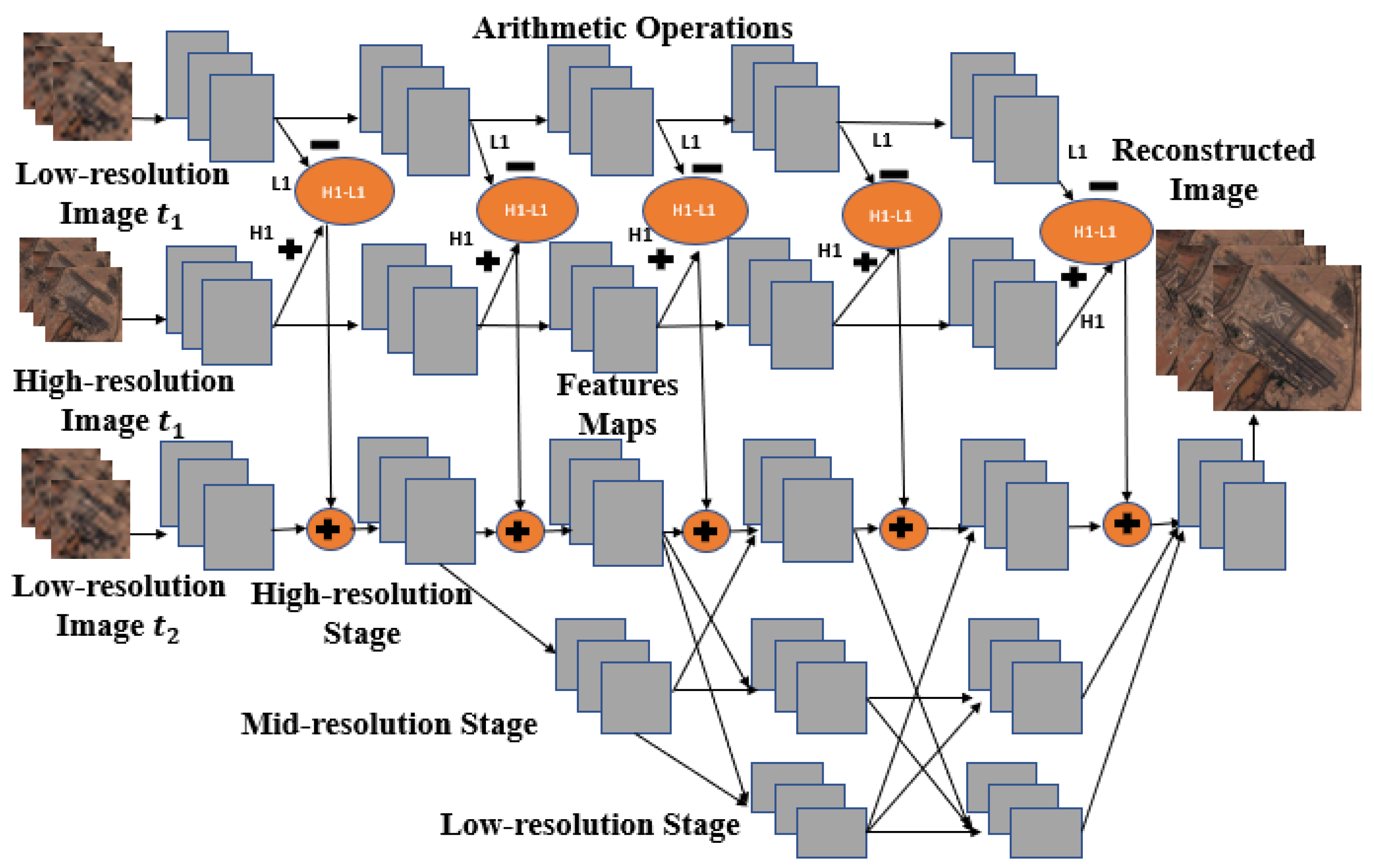
In the U-Net architecture, image feature maps are downsampled through polling to lower resolution in the encoder and upsampled in the decoder to match the input image size. High-resolution information is not kept in this downsampling and upsampling process; instead, high-resolution information is copied to the decoder through the skip connections. On the contrary, the HRNet architecture maintains all level resolution channels throughout the whole process during learning such that detailed information is better preserved in the reconstructed images. HRNet is now becoming the mainstream in many computer vision applications [34].
Figure 4 shows our proposed HRNet architecture. The model has five convolutional layers. Each layer is followed by a normalization layer and the ReLu activation function. It has three resolution stages, including high-, medium- and low-resolution, as shown in Figure 4. The high-resolution stage carries high-frequency information, which is crucial for sharper image generation, and the low-resolution stages account for large-scale contents in the images. The images in our experiments do not contain many large-scale changes between the two time points. As a consequence, arithmetic operations at lower-resolution stages may not provide much improvement. As the high-resolution stage carries high frequency information, we perform the same feature level arithmetic operations as those in the U-Net architecture in each convolutional layer at the high-resolution stage. We also conducted experiments by applying the arithmetic operations at all resolution stages. Nevertheless, only a marginal performance improvement was obtained with a significant increase in model complexity. Therefore, we chose this relatively simple structure. A similar histogram matching process is applied to all the images before training.

3.2. Loss Functions

To train the proposed fusion models, we used the popular mean-square error (MSE), and the well-recognized metric named high-frequency error norm normalized (HFENN) [35] as the cost function. The MSE metric is defined as:
M S E = 1 W H C i = 1 W j = 1 H k = 1 C ( I i , j , k I ^ i , j , k )  
where I and I ^ denote the true and predicted high-resolution image at t 2 , respectively; and W, H, and C represent width, height, and number of channels in the images, respectively. The HFENN cost function is defined as:
H F E N N = L o G I L o G I ^   L o G I ^
where LoG denotes the Laplacian of the Gaussian operator, which captures high-frequency information in the fused images [36]. The total cost function used in our study is then defined as the combination of the two.
L = MSE + 10 × HFENN
We put a larger weight (10–based on experiments) on HFENN such that the model can focus on high frequency details. The total loss function L not only tells of the pixel-wise difference between two images in general, but also puts more emphasis on high-frequency component differences between the two images.

3.3. Performance Metrics

We used five performance metrics to evaluate different models in our study, including peak signal to noise ratio (PSNR), structural similarity (SSIM), spectral angle mapper (SAM), relative dimensionless global error (ERGAS), and root-mean square error (RMSE) [36,37]. These metrics are defined as follows:
P S N R = 10   log   ( R 2 M S E )
where R is the maximum range of input image data type. A higher PSNR value indicates a better image quality for the reconstructed high-resolution image.
S S I M = 2 μ 1 μ 2 + L 1     2 Φ I I ^ + L 2   μ I 2 + μ I ^ 2 + L 1   Φ I   2 + Φ I ^   2 + L 2
where μ 1 and μ ^ represent mean pixel values of ground truth and its predicted image, Φ I I ^ denotes covariance between ground truth and the predicted image, and L 1 and L 2 are predefined constants. A higher value of SSIM also indicates better image quality.
S A M = 1 N i = 1 N a r c c o s j = 1 C I i j   I ^ i j   j = 1 C ( I ^ i j ) 2 k = 1 C I i k 2
where N indicates the total number of pixels in the fused image and C is the number of bands in the image. The SAM metric is used to measure spectral distortion of an image. A small value indicates better image quality.
R M S E = ( 1 H W C   i = 1 H j = 1 W k = 1 C ( I i , j , k   I ^ i , j , k   )   )  
E R G A S = 100 * l h 1 C i = 1 C R M S E ( I ) 1 2 μ i
where h and l denote spatial resolutions of high- and low-resolution images, respectively. RMSE is used to calculate global radiometric difference between ground truth and the fused image. ERGAS is used to evaluate the quality of a fused image based on the normalized average error of each band in the processed image. Smaller values of RMSE and ERGAS represent better image quality.

4. Experimental Setup

4.1. Datasets

We utilized WV-2, Sentinel-2, Landsat-8, and NAIP images to evaluate the proposed fusion model. Details of these imagery systems and data for both training and testing are listed in Table 1 and Table 2. For WV-2 images, the study area covered the Millerovo airport, which is located in Russia; and the images contain airplanes, buildings, vegetation, etc. We collect cloud-free images at two time points (04/2014 and 07/2015) with image resolution of 0.46 m for training.
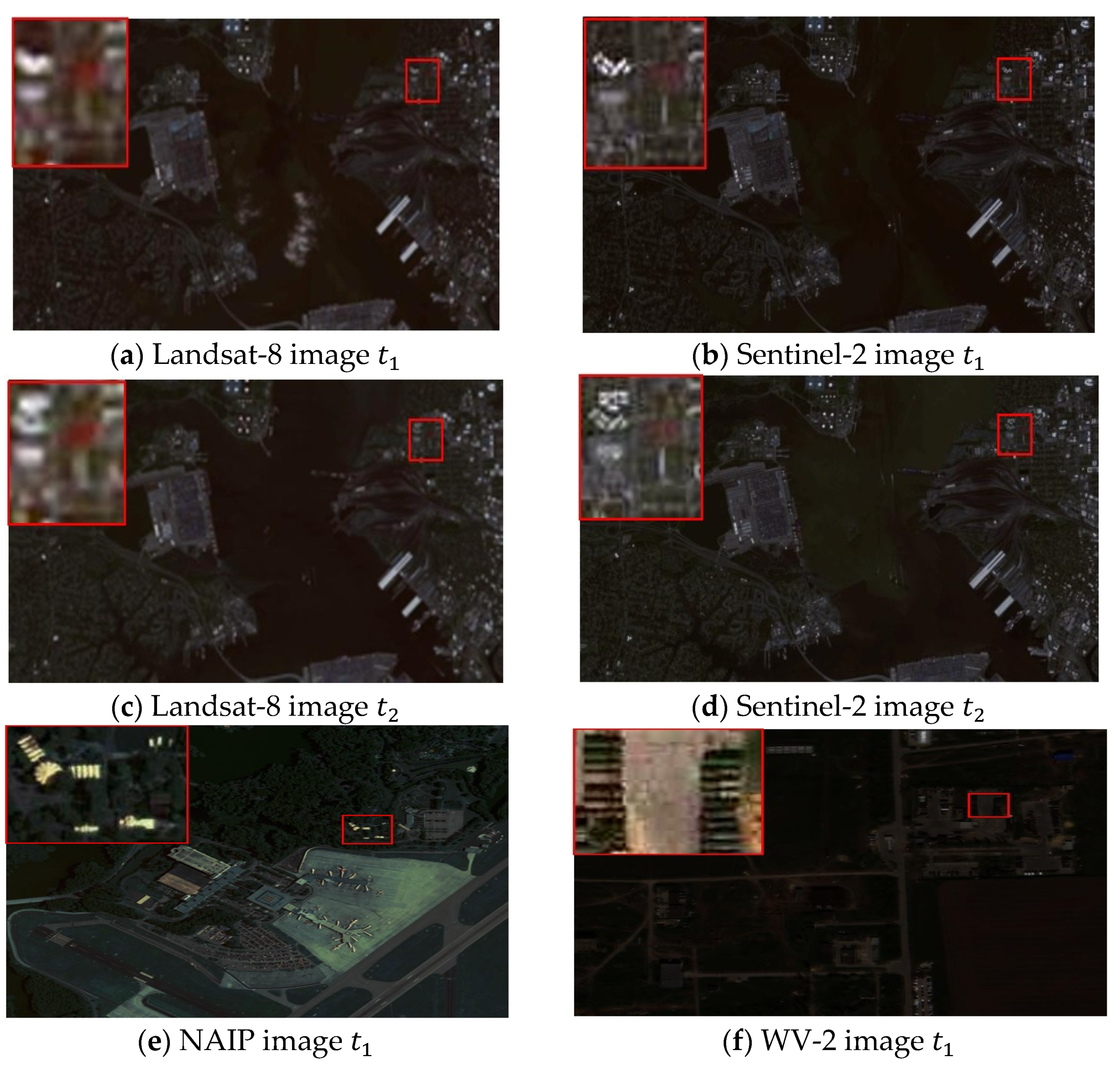
For NAIP, Sentinel-2 and Landsat-8 images, we choose Norfolk, VA, as our study area due to the rapid urban development over time in this region. Figure 5 shows some training image pairs used in this study. Image resolutions of NAIP, Sentinel-2, and Landsat-8 images are 1, 10, and 30 m, respectively.
For evaluation, we chose 20 smaller images with different dimensions in the adjacent area for each of the experiments. The time difference between the two time points was about two years. Significant temporal changes can be observed between the image pairs. In addition, we collected 45 testing images from Palm Jumeirah, Dubai, for testing the ability to generalize. This dataset consisted of low-resolution Landsat-8 images and paired high-resolution Sentinel-2 images. The time difference between the two time points was about four years, and significant temporal changes were present between image pairs.

4.2. Preprocessing

Different satellite images contain different numbers of channels. In this study, we only considered RGB channels. As we apply arithmetic operations to different images collected at different times, these images need to be registered. We utilized the projection distortion based on the control points method provided by Matlab R2020a (MathWorks Inc., Natick, MA, USA) for registration. We also performed data normalization and histogram matching for consistent performances.

4.3. Experiments

4.3.1. Experiment 1

We used the WV-2 dataset collected at the two time points for image fusion. We downsampled the images by averaging pixels with different factors (2×; 4×; 6×; 10×) to simulate low-resolution images at both time points, making the low- and high-resolution images at the same time point perfectly registered. We expect better performances than other experiments where the images registration was not perfect. This experiment tested the upper limit on the number of times the high-resolution images can be downsampled while still achieving good fused high-resolution images.

4.3.2. Experiment 2

Landsat-8 images have a resolution of 30 m, and Sentinel-2 images have a resolution of 10 m. The images collected from Norfolk, VA, are of around two years apart. We fused Landsat-8 and Sentinel-2 images at t 1 with Landsat-8 images at t 2 to generate Sentinel-2 images at t 2 . There is a factor of 3× difference in resolutions between the two image datasets, and we expected good performances, though the registration is not perfect.

4.3.3. Experiment 3

Sentinel-2 images have a resolution of 10 m, and NAIP images have a resolution of 1 m. The images collected from Norfolk, VA, are of around two years apart. We fused Sentinel-2 images and NAIP images at t 1 with Sentinel-2 images at t 2 to generate NAIP images at t 2 . This was the most challenging task in our study due to a resolution difference of 10× between the two different modalities. We tested the proposed fusion model on this dataset with an imperfect registration.

4.3.4. Experiment 4

To evaluate generalization capability of the proposed models, we applied models trained with data collected in Norfolk, VA, USA, to data collected in Palm Jumeirah in Dubai without fine-tuning. Palm Jumeirah has been experiencing rapid growth of urbanization over the past few years. The time gap between the image pairs we collected is about 4 years, and significant temporal changes are present in the image pairs. Low-resolution images captured by Landsat-8 have 30 m resolution, and the high-resolution images were from Sentinel-2 with a resolution of 10 m.

4.3.5. Experiment 5: Statistical Tests

We performed two statistical (parametric and non-parametric) tests to show if performance differences between the proposed model (best) and the best baseline model are significant. Parametric tests are performed when the data size is large and the data are normally distributed, whereas non-parametric tests are conducted if data size is small and the data do not assume a normal distribution [38]. For parametric test, we applied the two-sample t-test, and for non-parametric test, we performed the Wilcoxon rank sum test. Both tests assume the involved samples are independent [39].

4.4. Competing Methods and Abbreviations

Our proposed model can combine different backbones and loss functions, resulting in four methods: “U-Net + MSE” (UMSE), “U-Net + MSE + HFENN” (UMSEh), “HRNet + MSE” (HMSE), and “HRNet + MSE + HFENN” (HMSEh). We also compared our model to the ATPRK method [19]; and the deep models ESRCNN [12], GAN [32], and STFGAN [40]. For the implementations of ESRCNN, GAN, and STFGAN, we followed the same settings utilized in the original papers and combined all temporal images to form inputs (similar to our proposed models) for fair comparisons.

5. Results and Discussion

5.1. Hyperparameter Determination

In all of the five experiments, we set input image patch dimensions to 32 × 32 × 3, convolutional kernel size to 3 × 3, batch size to 32, and number of training epochs to 35. We included five convolutional layers in both the U-Net and HRNet backbones, where each convolutional layer was followed by a batch normalization layer and the ReLu activation. We fixed the dropout rate to 0.1 for all dropout layers and used the Adam optimizer during training with default learning rates. All models were trained on a high-performance computing cluster (GPU, 128 GB RAM, 16 cores). The model was implemented using the Keras platform [41].

5.2. Results and Analysis

5.2.1. Results of Experiment 1 and Analysis

Table 3 shows performance metrics by different models with which we downsampled the high-resolution WV-2 images as perfectly registered low-resolution images for fusion. We tested four down-sampling factors, including 2×, 4×, 6×, and 10×, and compared the proposed models with ATPRK, ESRCNN, and GANs (GAN, STFGAN). The ATPRK model showed consistently poor performances for all cases. ESRCNN produced competitive results for the 2× case and achieved the best SAM of 2.48. However, for most of the other cases, the proposed model with the U-Net and HRNet backbone model achieved better results.
If images are perfectly registered (Experiment 1), our proposed models can handle up to 12× spatial resolution differences (PSNR of UMSE reached 40.30 dB at 10× downsampling) and carry temporal changes to the fused high-resolution images. The U-Net backbone outperforms the HRNet backbone in most of all the metrics for 10× and 4×. For 6× and 2×, the HRNet backbone outperforms the U-Net backbone (Table 3). However, we shows (in Section 5.2.8) that the HRNet backbone retained more details in the fused image, making it much sharper. These performance metrics may not be ideal to capture high-frequency details [42] in images, and better matrices are desired. Our proposed model shows the potential to fuse different remote image modalities in practice. The competing method, ARPRK, failed to generate a sharp image, and ESRCNN failed to capture temporal changes. Neither of them achieved a sharp image with proper temporal changes at the same time. The GAN model produced sharp images in Experiment 1 but quantitatively did not perform well (GAN, STFGAN) and failed the fusion task in Experiment 3, unlike our proposed models.

5.2.2. Results of Experiment 2 and Analysis

Table 4 shows results of fusing Landsat-8 images to generate high-resolution Sentinel-2 images; the resolution difference was 3×. The proposed models achieved better results (all other cases) than the competing methods (ATPRK, ESRCNN, and GANs) in terms of all the five metrics. The model with the U-Net backbone and the high frequency loss (UMSEh) outperformed the HRNet-backbone model in all metrics except SAM.
The resolution difference between Sentinel-2 and Landsat-8 is 3× (10 m vs. 30 m), and the fusion results visually look good. However, the best PSNR dropped to 29.55 dB (by UMSEh), as compared to the best case at 4× in Experiment 1 (42.16 dB by UMSEh), partially because the image registration was imperfect. However, the temporal changes were captured nearly perfectly (described in Section 5.2.7), The fused images ideally will have a 10 m spatial resolution and are suitable for large object detection, including that of boats, buildings, etc. Since both of the modalities are free of charge, they have potential for practical nonessential applications.

5.2.3. Results of Experiment 3 and Analysis

Image fusion results from Sentinel-2 to NAIP are listed in Table 4, where the resolution difference is 10× and image registration of the two modalities differs (satellite and aerial) and is imperfect. The proposed method with U-Net as a backbone and MSE + HFENN as loss functions (UMSEh) won by four out of the five performance metrics. Both GAN models did not perform well. Surprisingly, the ATPRK model performed better than ESRCNN. In summary, from Table 4, it is clear that the proposed model achieved the best overall results.
NAIP provides very-high-resolution (1 m) time-series images; it is designed for agriculture application monitoring. One limitation is that NAIP is not free of charge. As shown in Table 4, the PSNR of the fused images from free Sentinel-2 images can reach 12.37 dB by UMSEh. However, they are still not clear and need further investigation if the fused images are to be used for agriculture monitoring applications. As compared to Experiment 2, the resolution difference in Experiment 3 was 10×, along with the two different modalities (Sentinel-2: satellite, NAIP: aerial), so that it is not surprising that the PSNR performance metrics dropped significantly.

5.2.4. Results of Experiment 4 and Analysis

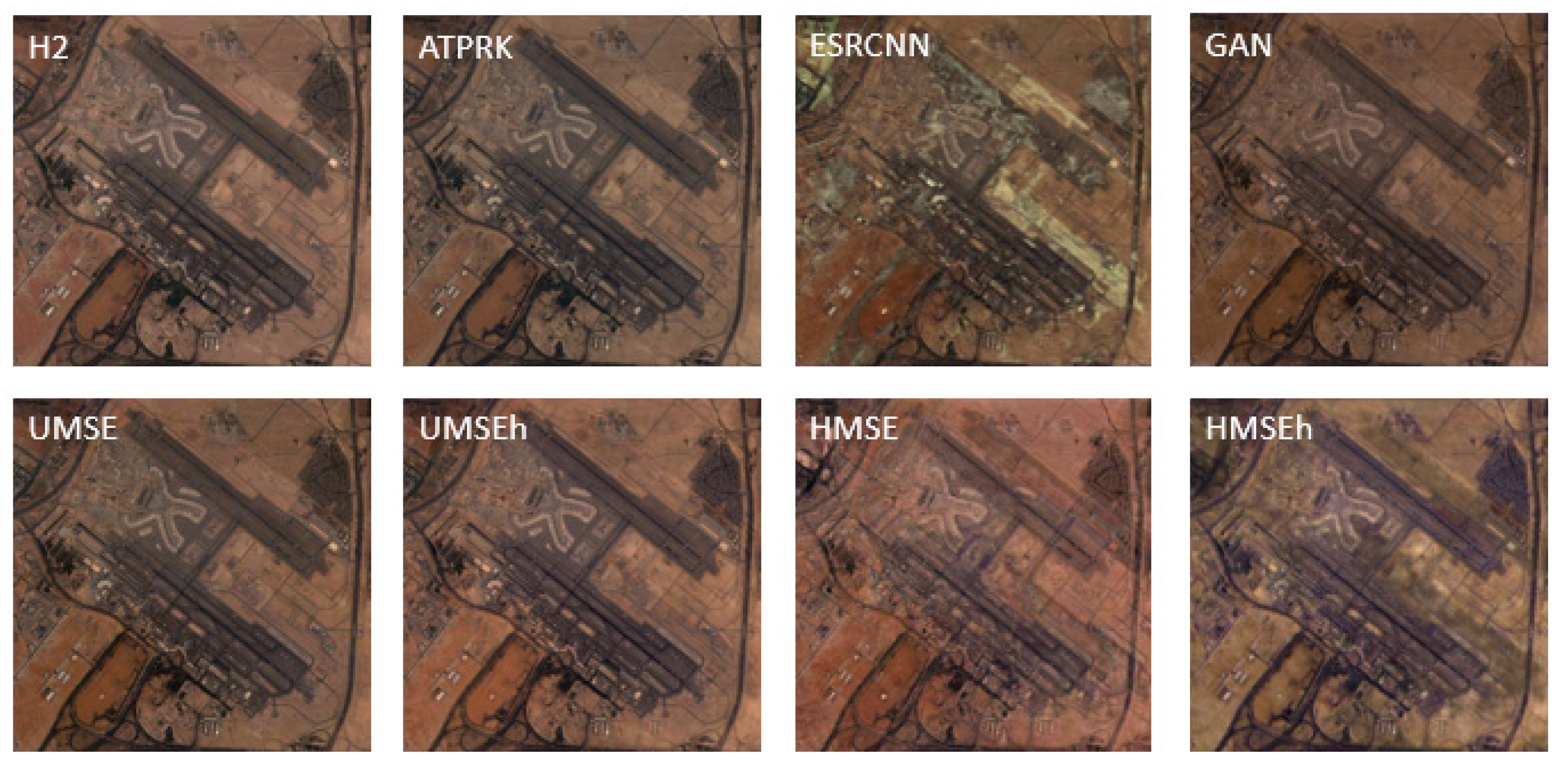
Table 5 shows transfer learning performances of the proposed models trained with data collected in Norfolk, VA, and applied to data collected in Palm Jumeirah. The objective of the fusion was to generate high-resolution Sentinel images from low-resolution Landsat-8 images for two-time points with temporal changes. Our proposed models achieved the best performances in all five metrics as compared to ATPRK, ESRCNN, and GANs. In particular, the U-Net backbone with high-frequency loss (UMSEh) achieved the best PSNR, SSIM, and RMSE. The HRNet bone with regular loss obtained the best SAM and ERGAS. Figure 6 shows some of the fused images in the Palm Jumeirah area. Quantitatively, STFGAN is similar to GAN; GAN performed slightly better. We only show the results by GAN for all the experiments to save space. Visual inspection shows that GAN and U-NET backboned models performed well. The color contrast in images produced by other computing methods (ESCNN, HMSE, HMSEh) does not match that in the ground truth image (H2).

5.2.5. Results of Statistical Tests

We performed statistical tests between the proposed model UMSEh and GAN. UMSEh achieved the overall best results, and GAN was the best baseline model for all of our experiments, as shown in Table 6. For Experiment 1, we report the statistical test for the 4× resolution case. Table 6 shows that UMSEh is statistically better than GAN in terms of all cases, except for Experiment 3.

5.2.6. Visual Inspection

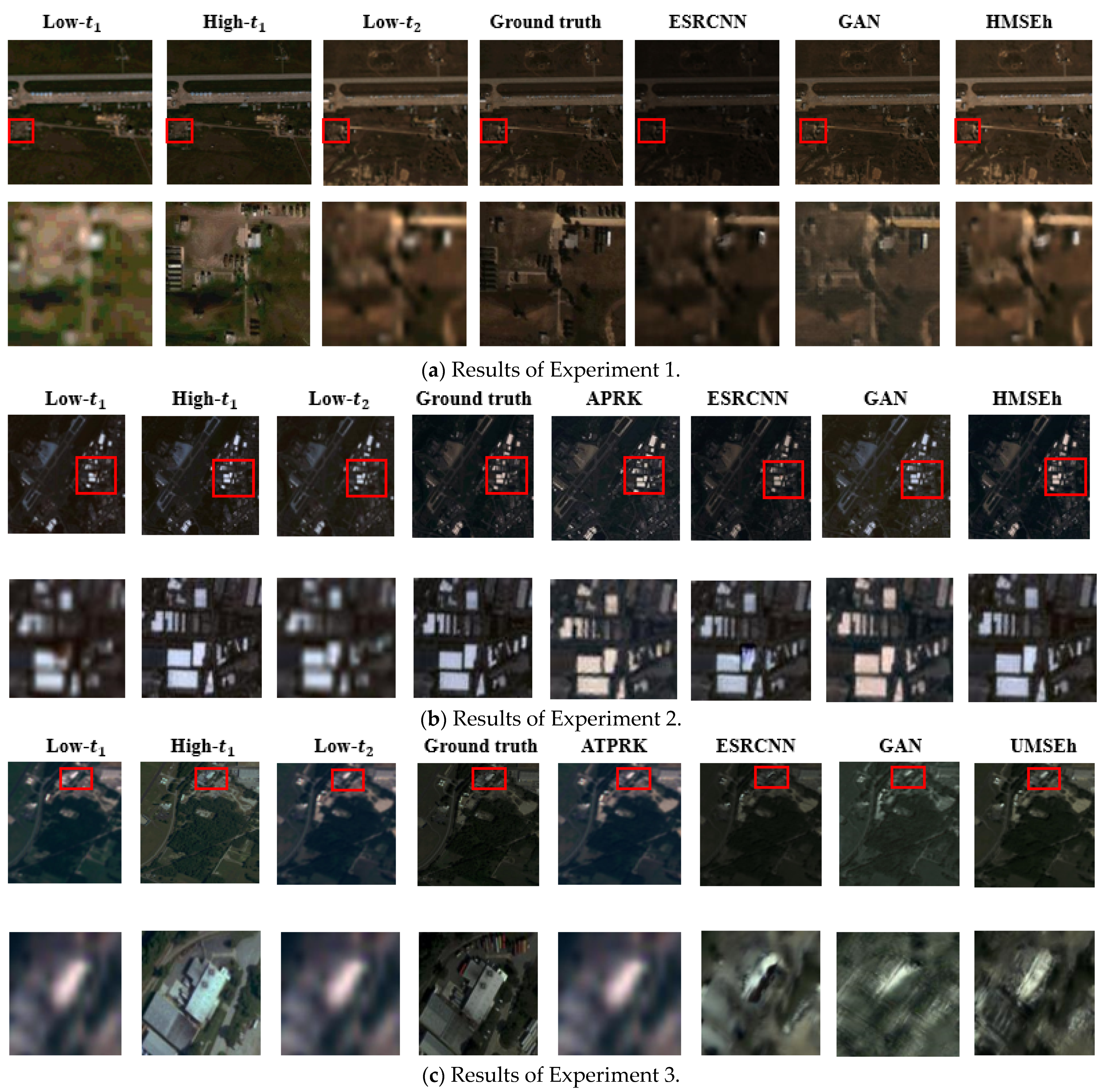
Figure 7 shows a fused testing image resulting from each of the experiments. The images fused by the ATRPK model (fifth column) are blurry, and the color contrast of some images does not match that of the ground truth (fourth column). The ESRCNN model generated images containing more details than these by ATPRK. The GAN model produced sharp outputs with visible details in Experiment 1 (Figure 7a), but performed the worst in Experiment 3 (Figure 7c). The proposed model produced much better results. Images generated by the HRNet-backbone model (HMSEh) are the sharpest by visual inspection.

5.2.7. Images with Temporal Changes

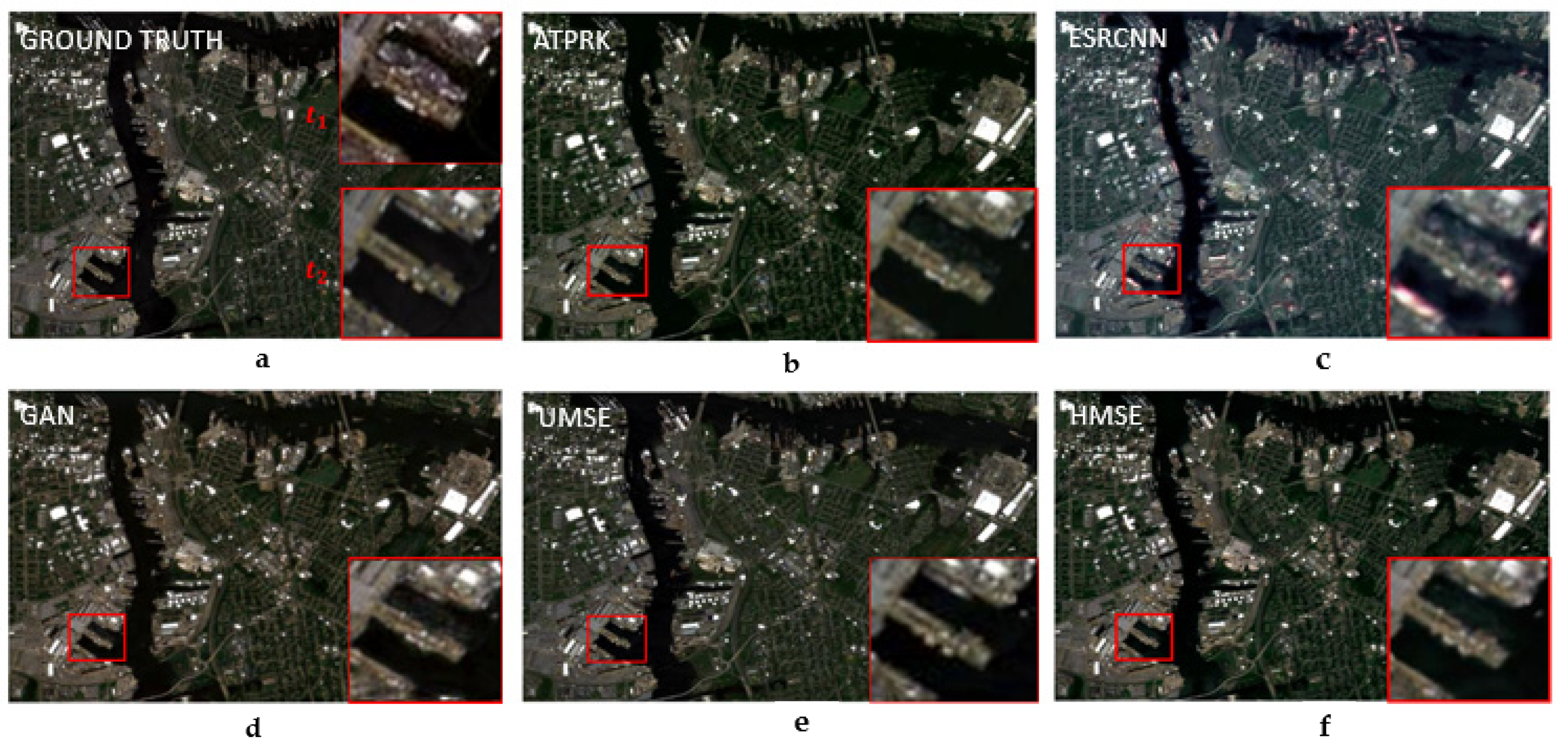
Figure 8 shows image fusion results when temporal changes are present in the Landsat-8 and Sentinel-2 dataset. The region is located inside the Norfolk port in Virginia, where a fleet was present at t 1 ,   and the fleet left at t 2 when the image was collected. The contour of the fleet is still visible in the image fused by the ESRCNN model (Figure 8c). Our proposed method with different loss functions and backbones (Figure 8e–f) clearly reflected the change. The ATPRK and GAN algorithms also successfully captured the temporal changes in the fused image.

5.2.8. Images with High-Frequency Details

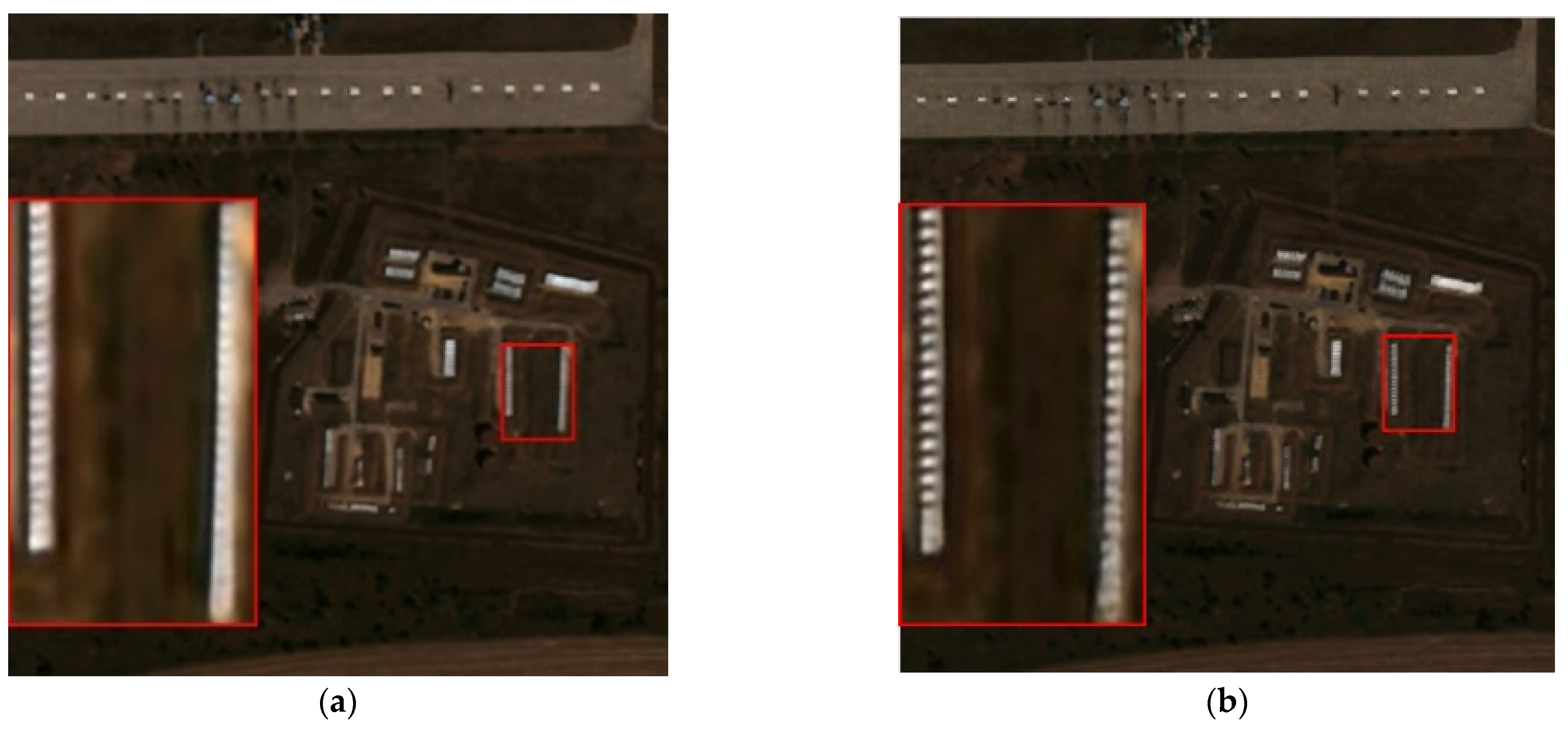
Figure 9 shows one fused image from Experiment 1 of 6× with high-frequency details inside the red square. It can be observed that the HRNet backbone (Figure 9b, HMSEh) can better keep these high-frequency details as compared to the U-Net backbone (Figure 9a, UMSEh), producing sharper details.

5.2.9. Upper Limit of the Downsampling Factor

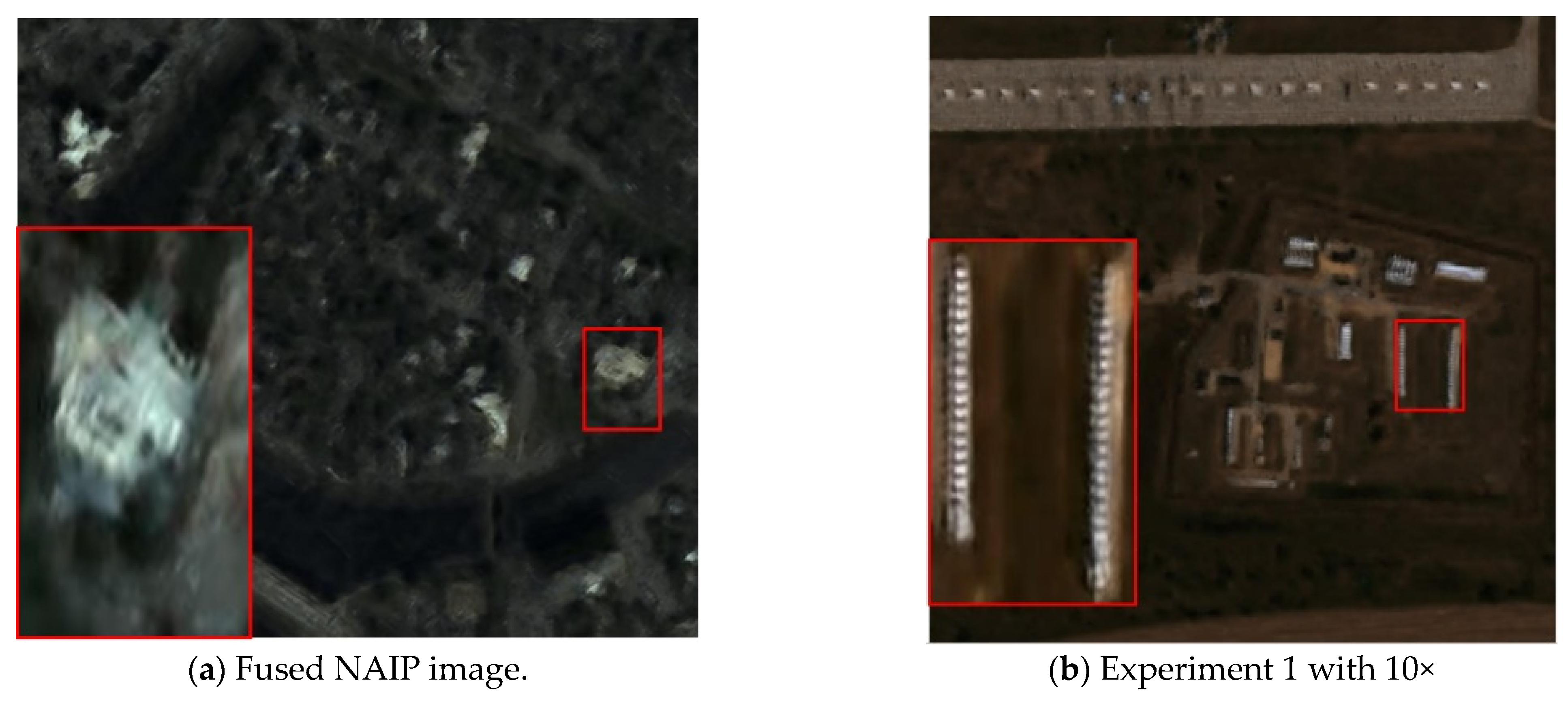
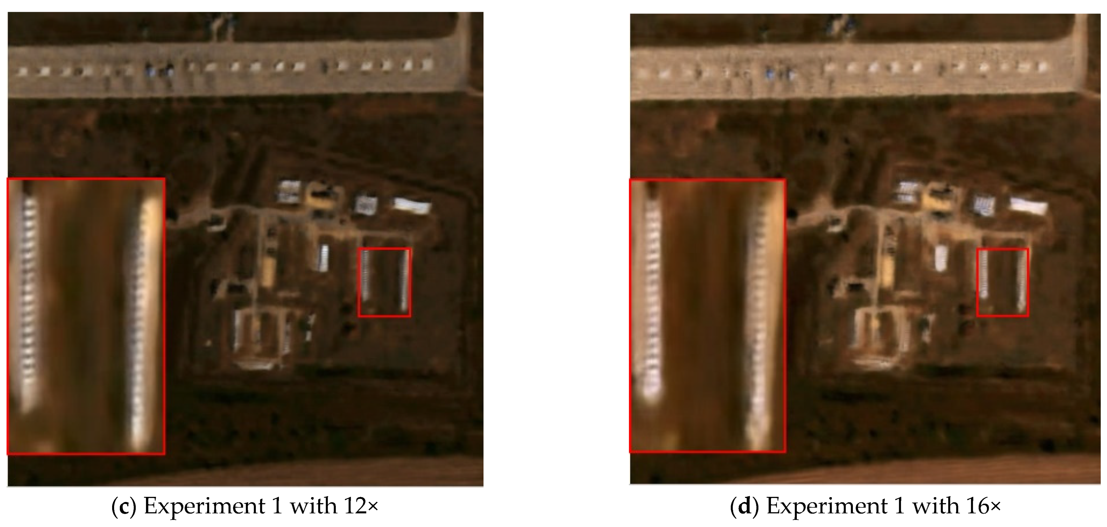
We performed experiments on the WorldView-2 dataset to investigate the extent that an image may be downsampled while still achieving good fused images, given that the image registration is perfect. We continued to downsample the image with factors of 12× and 16× and applied the proposed model for image fusion. Figure 10b–d show the fused images with factors 10×, 12×, and 16×, respectively. It can be observed that the fused image with the factor of 16× is blurry, and we conclude that the upper limit may be 12×, which is our proposed limit.

6. Discussion

For environmental monitoring or land surface change detection, a remote sensing imaging system that can densely sample a particular region with high spatial resolution is desired. The proposed model is an attempt to fuse multiple satellite image modalities to generate high resolution in both temporal and spatial domains.
Our proposed methods are simple yet fast (less than 2 min) and effective at capturing temporal changes. We unitized arithmetic operations in feature space to achieve this goal. In the encoder parts of U-Net and HRNet, we subtracted features of low-resolution images from features of high-resolution images at t 1 and added features of low-resolution images at t 2 . These low-resolution features represent contours, and high-resolution features represent both contours and detail texture information in the images. We utilized these arithmetic operations to explicitly reflect low-resolution temporal contour changes. Though high-resolution information was not provided at the input, we assumed that high-resolution texture information would be correlated with shapes of contours and could be learned from similar texture patches in training data so that the changed contours at t 2 can be correctly filled with details. We expect direct deep learning models such as ESRCNN will eventually learn the arithmetic relationship between the three inputs and output and correctly reflect temporal changes, if more data are provided. The explicit arithmetic feature operations guided the training and made the learning much easier, which will be further investigated in our future work.
In general, our proposed models are capable of accurately capturing temporal changes while enhancing spatial resolution. These results were confirmed by both the performance metrics and visual inspection. ATRPK can also capture such changes, but the generated images are blurry, and image contrast sometimes does not match that of ground truth. ESRCNN can preserve image contrast, but the fused images cannot update temporal changes. GANs can catch temporal changes, but they also have the image contrast mismatch issue, and this failed in Experiment 3. It is worth noting that our models heavily depend on image registration. Perfect registration can tolerate a spatial resolution difference of up to 12× during fusion (Figure 10).
Though the proposed U-Net backbone quantitatively outperformed the HRNet backbone in many cases, the metrics we used for performance evaluation are based on MSE regression-based techniques, which compare features on pixel basis and penalize any synthetic high-frequency detail that is not perfectly aligned with the ground-truth image [42].
Visually, the HRNet backbone generated sharper images, and the details in the generated images are much sharper than those in the U-Net generated images, because the HRNet backbone models maintain high resolution throughout the whole learning process, and can capture high-frequency components better than U-Net. Images fused by the ATPRK model are usually blurry. ESRCNN and GANs were also outperformed by the U-Net and HRNet backbone models in most cases.

7. Conclusions and Future Research

We proposed an arithmetic deep image fusing method, ArithFusion, for multimodal temporal remote sensing image fusion. We applied it to Landsat-8, WorldView-2, Sentinel2, and NAIP satellite image pairs in this study. ArithFusion with both the U-Net and HRNet backbones achieved better results as compared to the traditional method (ATPRK) and the deep models (ESRCNN, GAN, STFGAN). While HRNet obtained similar performance metrics to U-Net, the images fused by HRNet are much sharper. GANs, ESRCNN, and ATPRK either cannot catch temporal changes, or the fused images are blurry. ArithFusion successfully tackled these two challenges, making it a suitable candidate tool for fusing multimodal temporal remote sensing images to be leveraged by other applications.
In this paper, we focused only on RGB fusion because there are many applications for which such images are sufficient. For example, references [43,44] and references therein include some applications that only use RGB images.
Although we focused on cloud and shadow-free RGB image fusion in this paper, the proposed methodology, in principle, is applicable to multispectral images. It should be noted that multispectral fusion between different satellite images requires the wavelengths of bands to be compatible. For instance, Sentinel-2 and Landsat-8 have somewhat different bandwidths and radiometric conditions at different bands. To fuse those bands with different bandwidths and to cover all sky conditions for image fusion, some special considerations need to be taken into account, which will be a future research direction.

Author Contributions

Conceptualization M.R.U.H. and J.L.; methodology, M.R.U.H. and J.L.; software, M.R.U.H. and J.L.; data curation, M.R.U.H., J.L., C.K. and K.K.; writing—original draft preparation, M.R.U.H. and J.L.; writing—review and editing, J.W. and C.K. All authors have read and agreed to the published version of the manuscript.

Funding

This research received no external funding.

Data Availability Statement

Our source code and data can be found from the following link: https://github.com/reshadshuvo123/Image-fusion.

Acknowledgments

We sincerely thank Adam Stavola for his careful proofreading of the manuscript.

Conflicts of Interest

The authors declare no conflict of interest.

References

  1. Shen, M.; Tang, Y.; Chen, J.; Zhu, X.; Zheng, Y. Influences of temperature and precipitation before the growing season on spring phenology in grasslands of the central and eastern Qinghai-Tibetan Plateau. Agric. For. Meteorol. 2011, 151, 1711–1722. [Google Scholar] [CrossRef]
  2. Amoros-Lopez, J.; G’omez-Chova, L.; Alonso, L.; Guanter, L.; Zurita-Milla, R.; Moreno, J.; Camps-Valls, G. Multitemporal fusion of landsat/tm and envisat/meris for crop monitoring. Int. J. Appl. Earth Obs. Geoinf. 2013, 23, 132–141. [Google Scholar] [CrossRef]
  3. Liao, C.; Wang, J.; Dong, T.; Shang, J.; Liu, J.; Song, Y. Using spatio-temporal fusion of landsat-8 and modis data to derive phenology, biomass and yield estimates for corn and soybean. Sci. Total Environ. 2019, 650, 1707–1721. [Google Scholar] [CrossRef] [PubMed]
  4. Johnson, M.D.; Hsieh, W.W.; Cannon, A.J.; Davidson, A.; Bedard, F. Crop yield forecasting on the Canadian prairies by remotely sensed vegetation indices and machine learning methods. Agric. For. Meteorol. 2016, 218, 74–84. [Google Scholar] [CrossRef]
  5. Yang, X.; Lo, C. Using a time series of satellite imagery to detect land use and land cover changes in the Atlanta, Georgia metropolitan area. Int. J. Remote Sens. 2002, 23, 1775–1798. [Google Scholar] [CrossRef]
  6. Li, X.; Zhou, Y.; Asrar, G.R.; Mao, J.; Li, X.; Li, W. Response of vegetation phenology to urbanization in the conterminous united states. Glob. Chang. Biol. 2017, 23, 2818–2830. [Google Scholar] [CrossRef]
  7. Hilker, T.; Wulder, M.A.; Coops, N.C.; Seitz, N.; White, J.C.; Gao, F.; Masek, J.G.; Stenhouse, G. Generation of dense time series synthetic Landsat data through data blending with modis using a spatial and temporal adaptive reflectance fusion model. Remote Sens. Environ. 2009, 113, 1988–1999. [Google Scholar] [CrossRef]
  8. Ranson, K.; Kovacs, K.; Sun, G.; Kharuk, V. Disturbance recognition in the boreal forest using radar and landsat-7. Can. J. Remote Sens. 2003, 29, 271–285. [Google Scholar] [CrossRef]
  9. Buying Satellite Imagery: Pricing Information for High Resolution Satellite Imagery. Available online: http://landinfo.com/satellite-imagery-pricing/ (accessed on 5 February 2021).
  10. Fu, P.; Weng, Q. Consistent land surface temperature data generation from irregularly spaced Landsat imagery. Remote Sens. Environ. 2016, 184, 175–187. [Google Scholar] [CrossRef]
  11. Zhu, X.; Cai, F.; Tian, J.; Williams, T. Spatiotemporal fusion of multisource remote sensing data: Literature survey, taxonomy, principles, applications, and future directions. Remote Sens. 2018, 10, 527. [Google Scholar] [CrossRef]
  12. Shao, Z.; Cai, J.; Fu, P.; Hu, L.; Liu, T. Deep learning-based fusion of landsat-8 and sentinel-2 images for a harmonized surface reflectance product. Remote Sens. Environ. 2019, 235, 111425. [Google Scholar] [CrossRef]
  13. Gao, F.; Masek, J.; Schwaller, M.; Hall, F. On the blending of the Landsat and modis surface reflectance: Predicting daily Landsat surface reflectance. IEEE Trans. Geosci. Remote Sens. 2006, 44, 2207–2218. [Google Scholar]
  14. Zhu, X.; Chen, J.; Gao, F.; Chen, X.; Masek, J. An enhanced spatial and temporal adaptive reflectance fusion model for complex heterogeneous regions. Remote Sens. Environ. 2010, 114, 2610–2623. [Google Scholar] [CrossRef]
  15. Shen, H.; Wu, P.; Liu, Y.; Ai, T.; Wang, Y.; Liu, X. A spatial and temporal reflectance fusion model considering sensor observation differences. Int. J. Remote Sens. 2013, 34, 4367–4383. [Google Scholar] [CrossRef]
  16. Zurita-Milla, R.; Clevers, J.G.; Schaepman, M.E. Unmixing-based Landsat tm and meris fr data fusion. IEEE Geosci. Remote Sens. Lett. 2008, 5, 453–457. [Google Scholar] [CrossRef] [Green Version]
  17. Zurita-Milla, R.; Kaiser, G.; Clevers, J.; Schneider, W.; Schaepman, M.E. Downscaling time series of meris full resolution data to monitor vegetation seasonal dynamics. Remote Sens. Environ. 2009, 113, 1874–1885. [Google Scholar] [CrossRef]
  18. Huang, B.; Song, H. Spatiotemporal reflectance fusion via sparse representation. IEEE Trans. Geosci. Remote Sens. 2012, 50, 3707–3716. [Google Scholar] [CrossRef]
  19. Song, H.; Huang, B. Spatiotemporal satellite image fusion through one-pair image learning. IEEE Trans. Geosci. Remote Sens. 2012, 51, 1883–1896. [Google Scholar] [CrossRef]
  20. Wang, Q.; Shi, W.; Atkinson, P.M.; Zhao, Y. Downscaling modis images with area-to-point regression kriging. Remote Sens. Environ. 2015, 166, 191–204. [Google Scholar] [CrossRef]
  21. Wang, Q.; Blackburn, G.A.; Onojeghuo, A.O.; Dash, J.; Zhou, L.; Zhang, Y.; Atkinson, P.M. Fusion of Landsat 8 oli and sentinel2 msi data. IEEE Trans. Geosci. Remote Sens. 2017, 55, 3885–3899. [Google Scholar] [CrossRef] [Green Version]
  22. Krizhevsky, A.; Sutskever, I.; Hinton, G.E. Imagenet classification with deep convolutional neural networks. Commun. ACM 2017, 60, 84–90. [Google Scholar] [CrossRef] [Green Version]
  23. Devlin, J.; Chang, M.-W.; Lee, K.; Toutanova, K. Bert: Pre-training of deep bidirectional transformers for language understanding. arXiv 2018, arXiv:1810.04805. [Google Scholar]
  24. Yang, L.; Zhang, M.; Li, C.; Bendersky, M.; Najork, M. Beyond 512 tokens: Siamese multi-depth transformer-based hierarchical encoder for long-form document matching. In Proceedings of the 29th ACM International Conference on Information & Knowledge Management, Online, 19–23 October 2020; pp. 1725–1734. [Google Scholar]
  25. Hannun, A.; Case, C.; Casper, J.; Catanzaro, B.; Diamos, G.; Elsen, E.; Prenger, R.; Satheesh, S.; Sengupta, S.; Coates, A.; et al. Deep speech: Scaling up end-to-end speech recognition. arXiv 2014, arXiv:1412.5567. [Google Scholar]
  26. Graves, A.; Mohamed, A.-r.; Hinton, G. Speech recognition with deep recurrent neural networks. In Proceedings of the 2013 IEEE International Conference on Acoustics, Speech and Signal Processing, Vancouver, BC, Canada, 26–31 May 2013; pp. 6645–6649. [Google Scholar]
  27. Petersson, H.; Gustafsson, D.; Bergstrom, D. Hyperspectral image analysis using deep learning—A review. In Proceedings of the 2016 Sixth International Conference on Image Processing Theory, Tools and Applications (IPTA), Oulu, Finland, 12–15 December 2016; pp. 1–6. [Google Scholar]
  28. Zhu, X.X.; Tuid, D.; Mou, L.; Xia, G.-S.; Zhang, L.; Xu, F.; Fraundorfer, F. Deep learning in remote sensing: A comprehensive review and list of resources. IEEE Geosci. Remote Sens. Mag. 2017, 5, 8–36. [Google Scholar] [CrossRef] [Green Version]
  29. Dong, C.; Loy, C.C.; He, K.; Tang, X. Image super-resolution using deep convolutional networks. IEEE Trans. Pattern Anal. Mach. Intell. 2015, 38, 295–307. [Google Scholar] [CrossRef] [PubMed] [Green Version]
  30. Song, H.; Liu, Q.; Wang, G.; Hang, R.; Huang, B. Spatiotemporal satellite image fusion using deep convolutional neural networks. IEEE J. Sel. Top. Appl. Earth Obs. Remote Sens. 2018, 11, 821–829. [Google Scholar] [CrossRef]
  31. Li, Y.; Li, J.; He, L.; Chen, J.; Plaza, A. A new sensor bias-driven spatio-temporal fusion model based on convolutional neural networks. Sci. China Inf. Sci. 2020, 63, 1–16. [Google Scholar] [CrossRef] [PubMed]
  32. Chen, B.; Li, J.; Jin, Y. Deep learning for feature-level data fusion: Higher resolution reconstruction of historical Landsat archive. Remote Sens. 2021, 13, 167. [Google Scholar] [CrossRef]
  33. Ronneberger, O.; Fischer, P.; Brox, T. U-net: Convolutional networks for biomedical image segmentation. In Proceedings of the International Conference on Medical Image Computing and Computer-Assisted Intervention, Munich, Germany, 5–9 October 2015; Springer: Cham, Switzerland, 2015; pp. 234–241. [Google Scholar]
  34. Wang, J.; Sun, K.; Cheng, T.; Jiang, B.; Deng, C.; Zhao, Y.; Xiao, B. Deep high-resolution representation learning for visual recognition. IEEE Trans. Pattern Anal. Mach. Intell. 2020, 43, 3349–3364. [Google Scholar] [CrossRef] [Green Version]
  35. Sun, L.; Fan, Z.; Ding, X.; Huang, Y.; Paisley, J. Region-of-interest undersampled mri reconstruction: A deep convolutional neural network approach. Magn. Reson. Imaging 2019, 63, 185–192. [Google Scholar] [CrossRef]
  36. Han, Y.; Du, H.; Lam, F.; Mei, W.; Fang, L. Image reconstruction using analysis model prior. Comput. Math. Methods Med. 2016, 2016, 7571934. [Google Scholar] [CrossRef] [PubMed] [Green Version]
  37. Vivone, G.; Alparone, L.; Chanussot, J.; Dalla Mura, M.; Garzelli, A.; Licciardi, G.A.; Restaino, R.; Wald, L. A critical comparison among pansharpening algorithms. IEEE Trans. Geosci. Remote Sens. 2014, 53, 2565–2586. [Google Scholar] [CrossRef]
  38. Vickers, A.J. Parametric versus non-parametric statistics in the analysis of randomized trials with non-normally distributed data. BMC Med. Res. Methodol. 2005, 5, 1–12. [Google Scholar] [CrossRef] [PubMed]
  39. Xu, M.; Fralick, D.; Zheng, J.Z.; Wang, B.; Tu, X.M.; Feng, C. The differences and similarities between two-sample t-test and paired t-test. Shanghai Arch. Psychiatry 2017, 29, 184. [Google Scholar]
  40. Zhang, H.; Song, Y.; Han, C.; Zhang, L. Remote sensing image spatiotemporal fusion using a generative adversarial network. IEEE Trans. Geosci. Remote Sens. 2020, 59, 4273–4286. [Google Scholar] [CrossRef]
  41. Keras. Available online: https://keras.io/ (accessed on 7 February 2020).
  42. Chitwan, S.; Ho, J.; Chan, W.; Salimans, T.; Fleet, D.J.; Norouzi, M. Image super-resolution via iterative refinement. arXiv 2021, arXiv:2104.07636. [Google Scholar]
  43. Ayhan, B.; Kwan, C. Tree, Shrub, and Grass Classification Using Only RGB Images. Remote Sens 2020, 12, 1333. [Google Scholar] [CrossRef]
  44. Ayhan, B.; Kwan, C.; Larkin, J.; Kwan, L.; Skarlatos, D.; Vlachos, M. Deep learning model for accurate vegetation classification using RGB image only. In Proceedings of the SPIE 11398, Geospatial Informatics X, Online, 27 April–8 May 2020. [Google Scholar]
Figure 1. Our proposed remote sensing image fusion approach.
Remotesensing 14 06160 g001
Figure 2. Diagram of the proposed deep learning fusion model.
Remotesensing 14 06160 g002
Figure 3. Proposed fusion model with the U-Net [33] backbone. In each of the convolutional feature maps, we subtract the low-resolution image’s features at t 1 (L1) from these extracted from the high-resolution image at t 1 (H1) and add these features computed from the low-resolution image at t 2 (L2) back into the feature maps to reconstruct the high-resolution image at t 2 .
Remotesensing 14 06160 g003
Figure 4. Proposed fusion model with the HRNet backbone [34]. In the high-resolution stage, we perform the same subtraction and addition arithmetic operations as those performed on the feature maps by the U-Net backbone model. We performed the arithmetic operations at all resolution stages. Nevertheless, only a marginal performance improvement was obtained for a significant increase in model complexity.
Remotesensing 14 06160 g004
Figure 5. Training image examples. Resolution: Landsat-8 (30 m), Sentinel-2 (10 m), NAIP (1 m), and WV-2 (0.46 m). Large red boxes display zoomed-in regions in the corresponding small boxes. Significant temporal changes can be observed. For example, in (e), the buildings are under construction and incomplete, whereas in (g), the buildings are completed. Image contrast was enhanced for better display.
Remotesensing 14 06160 g005aRemotesensing 14 06160 g005b
Figure 6. Image fusion results in Experiment 4 (transfer learning) by different methods, where H2 is the ground truth high-resolution image at the second time point. Image generated by ESRCNN contains noise; and histograms of images by HMSE, HMSEh, and GAN do not match that of the ground-truth image.
Remotesensing 14 06160 g006
Figure 7. Visual inspection of images fused by different models. (a) shows the results of the Experiment 1 where low- and high-resolution image pairs were downsampled by the 6× WV-2 image and its original version. (b) shows the results of Experiment 2 where low- and high-resolution image pairs are Landsat-8 and Sentinel-2 images. (c) shows the results of Experinet 3 where Low- and high-resolution image pairs are Sentinel-2 and NAIP images. For each of the experiment results, the first row shows input images and fused results by different models. “Low- t 1 ”, “High- t 1 ”, and “Low- t 2 ” are inputs images. “Ground truth” is the high-resolution image at t2. The second row shows the zoomed-in region in the red box above. Results of the proposed model are from the best combination of backbone and loss function in each of the experiments. Image contrast was enhanced for better display.
Remotesensing 14 06160 g007
Figure 8. Image fusion results with temporal changes. From left to right, the first row (ac) shows the ground-truth image, ATPRK, and ESRCNN; and the second row (df) shows GAN, UMSE, and HMSE, respectively. In the ground truth image, the zoomed-in regions at t 1 and t 2 show changes captured by the Sentinel-2 satellite image where a cargo ship docked in the Norfolk port at t 1 and left at t 2 . The ESRCNN failed to reflect the change in the fused image. ATPRK, GAN, and our models successfully captured this change in the fused images. UMSE: “U-Net + MSE”. HMSE: “HRNet + MSE”.
Remotesensing 14 06160 g008
Figure 9. Visual comparison for high-frequency details of images fused by the U-Net (a) and HRNet backbones (b). For this experiment we choose Experiment 1 with 6×. The large red box contains the zoomed-in region in the small box.
Remotesensing 14 06160 g009
Figure 10. Image registration effect. With imperfect registration in Experiment 3, the resolution difference of 10× between Sentinel2 and NAIP images is much more difficult to bridge (image in (a) is blurry). With the perfect registration in Experiment 1, even larger resolution differences resulted in much sharper fused images (bd).
Remotesensing 14 06160 g010aRemotesensing 14 06160 g010b
Table 1. Specifications of datasets used in the study.
SystemsModalityBandsResolutionRevisit FrequencyCharge
Landsat-8Satellite830 m16 daysFree
Sentinel-2Satellite1210 m10 daysFree
NAIPAerial41 m3 yearsVariable
WV-2Satellite80.46 mLess than 4 daysExpensive
Table 2. Details of training and testing data.
ExperimentsTypeDimensionNo. of Images
WV-2
(Experiment 1)
Training1024 × 1024 × 31
WV-2
(Experiment 1)
Testing200 × 300 × 3–700 × 800 × 320
Landsat-8 & Sentinel-2
(Experiment 2)
Training406 × 766 × 31
Landsat-8 & Sentinel-2
(Experiment 2)
Testing200 × 200 × 3–300 × 300 × 320
Sentinel-2 and NAIP
(Experiment 3)
Training1500 × 1500 × 31
Sentinel-2 and NAIP
(Experiment 3)
Testing100 × 200 × 3–500 × 800 × 320
Landsat-8 & Sentinel-2
(Experiment 4)
Testing100 × 200 × 3–400 × 600 × 345
Table 3. Results of Experiment 1. ATPRK, ESRCNN, and GANs are competing methods. All others are the proposed model with different backbones or different loss functions. Results are averages for 20 testing images and shown in the format of “mean (std)”. Best results are shown in bold.
MethodsScale-10×
PSNRSSIMSAMRMSEERGAS
ARPRK17.85 (5.75)0.48 (0.12)2.51 (0.40)34.27 (11.49)26.18 (3.45)
ESRCNN39.43 (3.49)0.95 (0.01)2.70 (0.77)2.91 (1.01)12.56 (2.88)
GAN36.87 (2.41)0.92 (0.01)4.01 (1.39)3.76 (0.77)14.26 (2.14)
STFGAN36.51 (1.69)0.93 (0.01)4.17 (1.28)3.96 (1.18)14.97 (3.72)
UMSE40.30 (2.91)0.96 (0.01)2.47 (0.55)2.58 (0.77)10.52 (2.22)
UMSEh40.05 (2.65)0.96 (0.01)2.71 (0.98)2.64 (0.74)10.66 (2.25)
HMSE38.80 (2.47)0.94 (0.01)2.94 (0.68)3.03 (0.78)14.77 (2.49)
HMSEh39.50 (2.77)0.95 (0.01)2.74 (0.64)2.82 (0.80)12.89 (2.30)
MethodsScale-6×
PSNRSSIMSAMRMSEERGAS
ARPRK19.32 (2.93)0.54 (0.13)2.31 (1.01)29.26 (11.43)24.69 (4.02)
ESRCNN40.93 (2.67)0.95 (0.01)4.97 (1.07)2.38 (0.64)10.29 (1.83)
GAN39.34 (1.85)0.93 (0.01)5.83 (1.27)2.80 (0.56)12.43 (1.90)
STFGAN40.54 (2.53)0.95 (0.01)4.17 (0.92)2.50 (0.88)10.43 (2.94)
UMSE40.65 (2.05)0.95 (0.01)5.16 (1.15)2.42 (0.53)10.24 (1.61)
UMSEh40.72 (2.62)0.95 (0.01)4.87 (1.08)2.43 (0.64)11.44 (1.76)
HMSE40.97 (2.17)0.95 (0.01)4.87 (1.15)2.35 (0.55)9.92 (1.72)
HMSEh41.14 (2.47)0.95 (0.01)4.99 (1.10)2.33 (0.59)9.98 (1.70)
MethodsScale-4×
PSNRSSIMSAMRMSEERGAS
ARPRK20.43 (2.92)0.58 (0.14)5.37 (1.06)26.32 (11.14)23.24 (4.61)
ESRCNN41.63 (2.56)0.95 (0.01)4.76 (0.99)2.19 (0.59)9.51 (2.19)
GAN39.73 (1.08)0.94 (0.01)5.67 (1.28)2.64 (0.34)11.43 (2.01
STFGAN39.63 (5.35)0.94 (0.06)4.45 (1.41)3.32 (3.08)13.29 (10.01)
UMSE41.87 (2.32)0.95 (0.01)5.02 (1.21)2.12 (0.55)10.31 (2.36)
UMSEh42.16 (2.54)0.96 (0.01)4.76 (1.14)2.06 (0.57)9.02 (2.04)
HMSE41.82 (2.38)0.96 (0.01)4.91 (1.16)2.13 (0.55)9.70 (2.09)
HMSEh40.32 (1.66)0.95 (0.01)4.91 (1.07)2.49 (0.45)13.04 (2.84)
MethodsScale-2×
PSNRSSIMSAMRMSEERGAS
ARPRK22.98 (3.42)0.68 (0.17)2.48 (0.90)19.71 (9.99)20.95 (6.19)
ESRCNN42.19 (2.53)0.97 (0.01)3.32 (0.71)2.06 (0.58)9.31 (2.22)
GAN39.90 (3.82)0.96 (0.01)4.33 (0.58)2.62 (1.11)13.33 (3.58)
STFGAN38.81 (4.34)0.96 (0.02)4.53 (1.55)3.24 (4.94)14.62 (4.81)
UMSE42.19 (2.53)0.97 (0.01)3.32 (0.71)2.02 (0.58)9.31 (2.22)
UMSEh42.16 (2.19)0.97 (0.01)3.29 (0.58)2.05 (0.53)8.71 (2.38)
HMSE41.41 (1.76)0.97 (0.01)3.77 (1.05)2.21 (0.46)10.95 (3.42)
HMSEh42.40 (2.54)0.98 (0.01)3.72 (1.00)2.01 (0.58)9.20 (2.39)
Table 4. Results of Experiment 2 (Landsat-8 and Sentinel fusion) and Experiment 3 (Sentinel and NAIP fusion). Results are averages of 20 testing images. Bold value indicates the best performance metric of a certain model.
MethodsExperiment 2
PSNRSSIMSAMRMSEERGAS
ARPRK23.40 (1.86)0.70 (0.07)6.81 (1.23)18.87 (4.00)19.57 (1.65)
ESRCNN27.34 (1.99)0.80 (0.04)5.91 (1.05)10.15 (2.61)15.83 (2.27)
GAN28.05 (1.74)0.82 (0.03)5.89 (1.03)9.36 (2.02)14.10 (0.89)
STFGAN28.28 (1.69)0.81 (0.04)5.90 (0.59)9.09 (1.88)14.02(0.88)
UMSE29.11 (1.95)0.83 (0.04)5.50 (0.79)9.12 (1.98)13.57 (1.02)
UMSEh29.55 (1.84)0.85 (0.03)5.95 (0.95)7.80 (1.74)12.84 (0.89)
HMSE28.64 (1.87)0.82 (0.04)5.39 (0.85)8.87 (2.06)13.95 (1.20)
HMSEh28.57 (1.91)0.82 (0.04)5.57 (0.64)9.41 (2.10)13.76 (1.25)
MethodsExperiment 3
PSNRSSIMSAMRMSEERGAS
ARPRK10.07 (3.90)0.22 (0.12)15.33 (6.63)84.81 (36.33)20.19 (7.85)
ESRCNN9.16 (1.68)0.14 (0.04)7.30 (2.54)96.25 (19.80)27.97 (9.20)
GAN10.72 (4.03)0.30 (0.11)5.55 (0.80)83.93 (37.27)17.79 (8.07)
STFGAN10.45 (2.70)0.30 (0.09)6.83 (1.13)80.05 (24.91)12.35 (3.86)
UMSE10.98 (2.52)0.22 (0.09)6.72 (2.17)79.68 (27.92)14.51 (5.53)
UMSEh12.37 (3.80)0.33 (0.11)5.95 (1.23)70.63 (35.97)10.62 (7.79)
HMSE11.72 (3.42)0.30 (0.10)5.54 (0.92)75.72 (33.64)13.90 (7.07)
HMSEh11.45 (2.99)0.23 (0.10)4.67 (0.65)78.62 (31.08)20.76 (6.21)
Table 5. Results of Experiment 4 (transfer learning). All models were trained with images collected from Norfolk, VA, and tested on images collected from Palm Jumeirah, Dubai. Results are averages of 45 testing images. Bold value indicates best performing value of a certain model.
MethodsPSNRSSIMSAMRMSEERGAS
ARPRK9.88 (1.37)0.14 (0.03)5.35 (1.63)82.71 (12.96)30.69 (1.47)
ESRCNN13.73 (0.75)0.31 (0.02)2.26 (0.50)52.62 (4.41)27.68 (0.51)
GAN13.74 (0.73)0.32 (0.02)2.45 (0.57)52.56 (4.28)27.66 (0.50)
STFGAN14.08 (0.93)0.31 (0.04)2.87 (1.25)50.66 (5.19)27.73 (0.69)
UMSE14.13 (0.63)0.33 (0.02)2.68 (0.41)50.24 (3.54)27.44 (0.54)
UMSEh14.50 (0.71)0.34 (0.02)2.55 (0.46)48.16 (3.82)27.44 (0.53)
HMSE14.17 (0.64)0.33 (0.03)2.23 (0.55)49.99 (3.57)27.42 (0.57)
HMSEh14.23 (0.63)0.33 (0.02)2.76 (0.48)49.63 (3.55)27.38 (0.55)
Table 6. Statistical tests between UMSEh (best overall) and GAN (best competing model) for all experiments, where h = 1 indicates the difference is significant at the 95% significance interval. Experiment 1 is for the 4× resolution case.
MetricsExperiment 1Experiment 2
Two Sampled T-TestWilcoxon Rank Sum TestTwo Sampled T-TestWilcoxon Rank Sum Test
p-Valuehp-Valuehp-Valuehp-Valueh
PSNR4.0 × 10 4 11.50 × 10 3 17.1 × 10 3 17.1 × 10 3 1
SSIM1.0 × 10 4 11.79 × 10 4 11.7 × 10 2 11.7 × 10 2 1
SAM2.2 × 10 2 11.03 × 10 3 19.1 × 10 1 09.1 × 10 1 0
RMSE4.0 × 10 4 11.50 × 10 3 17.8 × 10 3 17.8 × 10 3 1
ERGAS6.0 × 10 4 16.86 × 10 4 11.0 × 10 4 11.0 × 10 4 1
Experiment 3Experiment 4
MetricsTwo Sampled T-TestWilcoxon Rank Sum TestTwo Sampled T-TestWilcoxon Rank Sum Test
p-Valuehp-Valuehp-Valuehp-Valueh
PSNR2.60 × 10 1 01.13 × 10 1 03.42 × 10 6 11.18 × 10 6 1
SSIM4.10 × 10 1 03.89 × 10 1 02.48 × 10 5 16.69 × 10 6 1
SAM4.80 × 10 1 06.29 × 10 1 03.82 × 10 1 02.24 × 10 2 1
RMSE3.40 × 10 1 01.13 × 10 1 01.58 × 10 6 11.18 × 10 6 1
ERGAS1.06 × 10 1 06.50 × 10 2 11.56 × 10 4 11.82 × 10 5 1
Publisher’s Note: MDPI stays neutral with regard to jurisdictional claims in published maps and institutional affiliations.