Evapotranspiration Estimation with the S-SEBI Method from Landsat 8 Data against Lysimeter Measurements at the Barrax Site, Spain

Abstract

Evapotranspiration (ET) is a variable of the climatic system and hydrological cycle that plays an important role in biosphere–atmosphere–hydrosphere interactions. In this paper, remote sensing-based ET estimates with the simplified surface energy balance index (S-SEBI) model using Landsat 8 data were compared with in situ lysimeter measurements for different land covers (Grass, Wheat, Barley, and Vineyard) at the Barrax site, Spain, for the period 2014–2018. Daily estimates produced superior performance than hourly estimates in all the land covers, with an average difference of 12% and 15% for daily and hourly ET estimates, respectively. Grass and Vineyard showed the best performance, with an RMSE of 0.10 mm/h and 0.09 mm/h and 1.11 mm/day and 0.63 mm/day, respectively. Thus, the S-SEBI model is able to retrieve ET from Landsat 8 data with an average RMSE for daily ET of 0.86 mm/day. Some model uncertainties were also analyzed, and we concluded that the overpass of the Landsat missions represents neither the maximum daily ET nor the average daily ET, which contributes to an increase in errors in the estimated ET. However, the S-SEBI model can be used to operationally retrieve ET from agriculture sites with good accuracy and sufficient variation between pixels, thus being a suitable option to be adopted into operational ET remote sensing programs for irrigation scheduling or other purposes.

1. Introduction

Evapotranspiration (ET) represents the loss of water from the Earth’s surface to the atmosphere through the combined process of evaporation and transpiration. In general terms, the evaporation process occurs via open water bodies, bare soil, and plant surfaces, whereas the transpiration process occurs through vegetation or any other moisture-containing living surface [1]. Within the land–atmosphere interface, ET regulates the Earth’s energy and water cycles [1,2,3,4,5,6]. As a result, its estimation is critical to the ideal design and management of irrigation systems, efficient irrigation scheduling, and a wide variety of water resource management efforts [7]. Although ET represents an essential component of the hydrological cycle, it is one of the least understood. It is estimated that 60% of the precipitated water returns to the atmosphere through ET [8]. Nonetheless, because of the complex physical and biological controls on evaporation and transpiration in addition to different land cover properties, ET estimates may diverge substantially [9].

Conventional measurements of ET (i.e., sap flow, weighing lysimeter, pan measurement, Bowen ratio system, eddy covariance system) have a limited use because they are not spatially representative and also because of the dynamic nature of heat transfer processes [10,11,12]. Additionally, their employment is often expensive, time consuming, laborious, and sometimes subject to instrument failure [13]. Satellite remote sensing allows one to obtain large-scale ET, which can accordingly characterize the surface heterogeneity, ranging from individual pixels to an entire raster image. Hence, the combination of process-based models with remote sensing observations is a valuable strategy to quantify the spatio-temporal variations of ET. Accurate estimates of ET depend on the land surface temperature (Ts), solar radiation, albedo (α), and atmospheric conditions (e.g., transmissivity, downward radiation, cloud presence, etc.). In this context, various algorithms have been developed utilizing information from various types of remote sensing sensors. These approaches generally vary from purely empirical to physically based techniques derived from the surface energy balance (SEB) equation with different degrees of complexity, such as the Surface Energy Balance Algorithm over Land (SEBAL), the Mapping Evapotranspiration with Internalized Calibration (METRIC) model, the Surface Energy Balance System (SEBS), the Simple Algorithm for Evapotranspiration Retrieving (SAFER), the Simplified Surface Energy Balance Index (S-SEBI), the two-source model (TSM), and the two-source time-integrated model (TSTIM) [5,13,14].

Although many advances have been achieved in recent decades to accurately retrieve ET from satellite data, the validation of the final ET remains a troublesome issue, mainly due to both scaling effects (i.e., comparisons between remote sensing ET and ground-based ET measurements) and advection effects [15]. Discrepancies between modeled and observed components of ET indicate that the models may not be estimating the right values of total ET for the right physical reasons [16]. In addition, the conversion from instantaneous values (in watts) to daily or hourly values (in millimeters) is challenging, as it adds possible estimation errors. The S-SEBI method was originally proposed by Roerink et al. [6] to solve the SEB and retrieve ET from remote sensing. Afterward, Gómez et al. [17] and Sobrino et al. [4] extended the concept to map daily ET so that the sensible and latent heat flux (H and LE) are not calculated separately but through the evaporative fraction [17,18]. Unlike other methods that try to fix the temperature for wet and dry conditions for the whole image and/or for each land use class, the S-SEBI can estimate the SEB by considering the wet and dry conditions of the land surface. Furthermore, no additional meteorological inputs are required to run the model. Therefore, the S-SEBI is considered relatively simple to apply, which makes it appropriate for regions that lack in situ data and may guide the operational generation of continuous products for monitoring ET over agricultural areas.

The increasing pressure on water use is globally well known; at the same time, irrigation intensification is required to be increased for food production for a growing population [19]. Improving efficiency in techniques for monitoring water use, as well as regarding the validation of remote sensing-based models, is an immediate and current issue to be solved. It is fundamental to keep in mind that any empirical models should not be used indiscriminately without any modification or improvement to estimate ET from satellite data [15]. The S-SEBI has been already tested in different sites around the world by several researchers [17,18,20,21,22,23,24,25] and is reported as a simple and moderately accurate method to partition the SEB terms [4,6]. However, in most cases, the method has been evaluated with in situ flux data, such as eddy covariance (EC) measurements, which have energy balance closure errors that may reach 30% [26,27]. Therefore, differently from other in situ measurements that have known discrepancies, lysimeters are considered the ultimate standard for the measurement of ET, considering they are properly installed and managed [28]. In this paper, we explored the application of the S-SEBI model with Landsat 8 imagery against three different in situ lysimeters for the period of 2014–2018 at the Barrax site, Spain. We assessed the performance of the model under different land covers (Grass, Wheat, Barley, and Vineyard) and established a trusted validation for proper comprehension of the method potentialities in generating novel ET products for future satellite missions.

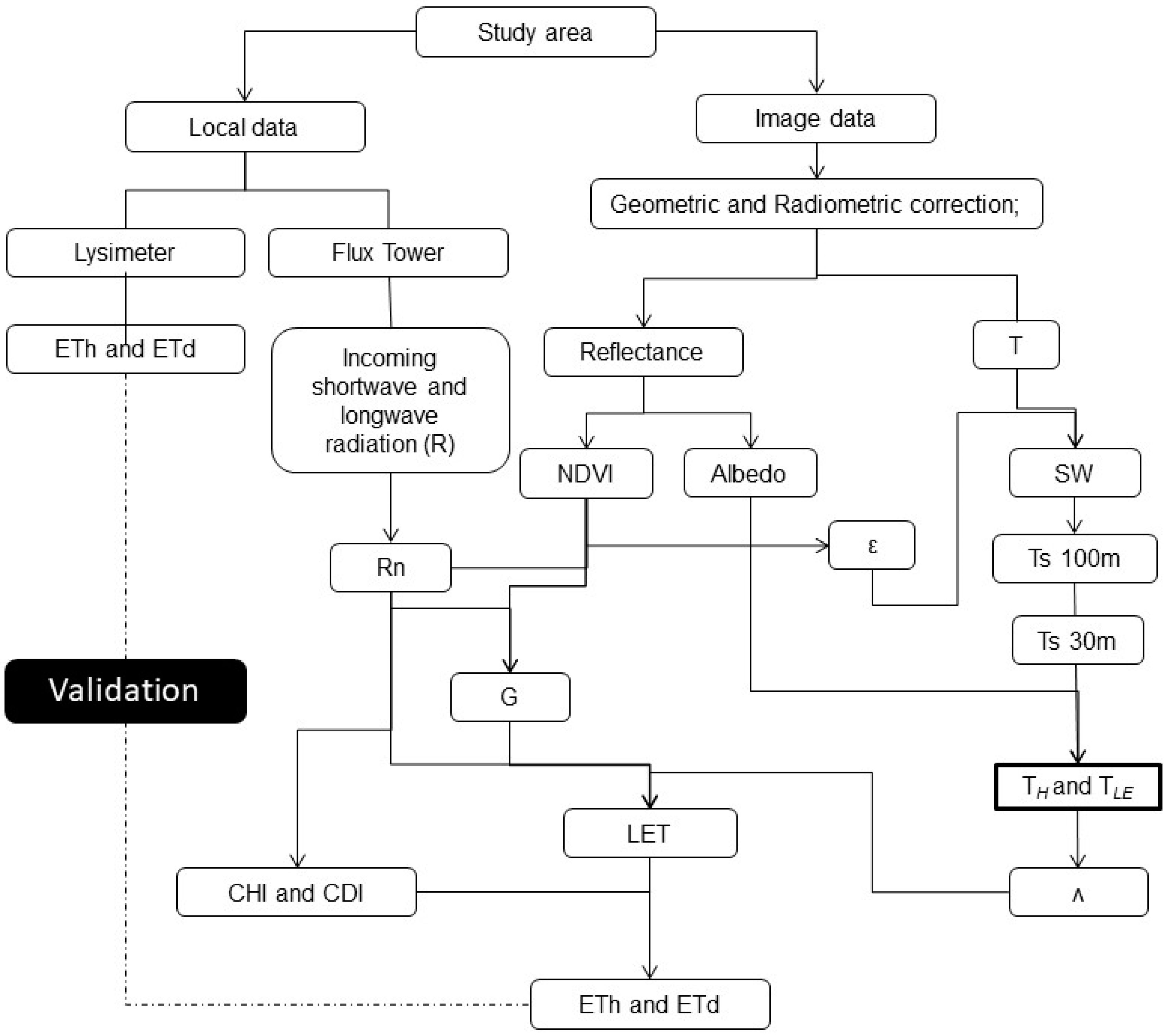
2. Methodology

In this section, the application and validation of the S-SEBI model using Landsat 8 images to an agricultural region in Spain (Barrax) are presented. Figure 1 shows the flowchart of the methodology applied.

The variables of the flowchart are presented in the next sections. In Figure 1, NDVI is the Normalized Difference Vegetation Index; T is the brightness temperature; SW is the split-window method; Ts is the land surface temperature; ε is the emissivity; Rn is the surface net radiation; G is the soil heat flux; T_H and T_LE are the temperatures corresponding to dry and wet conditions; LET is the latent heat flux; Λ is the evaporative fraction; C_di is the ratio between daily (R_d) and instantaneous (R_ni) net radiation flux; and C_hi is the ratio between hourly (R_hd) and instantaneous (R_ni) net radiation flux.

A disaggregation algorithm for Ts data was included because of a high spatial variability of the Barrax agricultural area and because we consider pixels of 100 m not representative of some small plots, such as Vineyard or Barley and Wheat, areas of which are less than 100 × 100 m. Disaggregation is recommended in order to retrieve a finer Ts pixel and more plot representation than a coarse Ts pixel, which can contain a mixture of different plots.

As the spatial resolution of thermal infrared pixels (100 m) is lower than visible/near-infrared (VNIR) data (30 m), a disaggregation method was applied to Ts in order to meet the spatial resolutions of albedo and NDVI variables. To do so, a linear relationship between Ts and NDVI in a sliding 5 × 5 pixel window was performed to retrieve the Ts pixel at 30 m, following the methodology proposed by Jeganathan et al. [29].

2.1. Study Area Description

This study was performed at the Barrax site located in the west of Albacete province, Spain. The site is a Mediterranean climate test area with the heaviest rainfalls in spring and autumn and the lowest in summer (Figure 2). The rainfall statistics show that the average annual rainfall is little more than 400 mm in most of the area, making La Mancha one of the driest regions in Europe [4,6,17,18,30,31,32,33]. The Barrax area has been selected in many field campaigns for calibration/validation activities because of its flat terrain and the presence of large, uniform land-use units (approximately 100 ha), suitable for validating moderate-resolution satellite image products.

2.2. In Situ Data

Barrax has a fixed station over a grass field with continuous land surface temperature (Ts) measurements taken by a radiometer that covers a footprint of 3 m² [34]. Besides Ts, this station provides other variables, such as wind direction and speed, soil flux, moisture and temperature, air temperature, and humidity, as well as net radiation. The net radiometer (model NR01) carries out separate measurements of solar (direct and reflected) and far infra-red (direct and reflected) radiations. A pyranometer measures the solar radiation flux from a field of view of 180° and has a spectral response from 0.3 μm to 2.8 μm. A pyrgeometer measures the far infra-red radiation flux from a field of view of 180° and has a spectral response from 4.5 μm to 50 μm.

The study area also has three continuous weighing lysimeters (see Figure 2) with electronic data readings: one lysimeter for Grass crops, one for rotating herbaceous crops (Wheat and Barley), and a permanent one for Vineyard. Each lysimeter is surrounded by a square protection plot of one hectare; the dimensions of the Grass and herbaceous crop lysimeter samples are 2.3 m 2.7 m to a side and 1.7 m depth with approximately 14.5 t total mass, and the Vineyard lysimeter sample is 3 m × 3 m to a side and 1.7m depth with 18.5 t total mass. The lysimeters have the necessary equipment to make a complete and accurate hydric balance as explained and tested by many authors [32,35]. The data are available in hourly measurements, which were used to validate the estimated ET calculated by the S-SEBI model between March 2014 and April 2018.

2.3. Satellite Data

We selected 62 Landsat 8 OLI/TIRS images to assess the efficiency of the S-SEBI model in estimating ET over different crops.

Table 1. Days of the year of the images used in this work for each land use.

Land Use	Day of the Year (DOY)
	2014	2015	2016	2017	2018
Grass	66; 75; 82; 98; 107; 123; 130; 146; 155; 162; 178; 194; 203; 219; 235; 251; 299; 306; 322	5; 14; 37; 69; 110; 126; 133; 158; 190; 213; 238; 270; 318; 334; 341; 357	8; 17; 24; 33; 65; 72; 273; 312; 337	83; 99; 122; 147; 163; 179; 218; 250; 282; 298; 314; 323; 330	22; 29; 54; 86; 109
Wheat	66; 75; 82; 98; 107; 123; 130; 146; 155; 162; 178
Barley				99; 122; 163; 170; 179
Vineyard	123; 130; 146; 155; 162; 178; 194; 203; 219; 226; 235; 251;	126; 133; 158; 190; 197; 222; 238; 245; 254; 270;	248; 273;	122; 163; 170; 179; 218; 250;

shows the days of years (DOYs) of the scenes used for each land cover and year evaluated. Grass has the largest amount of available in situ data for validation, thus being the land cover with more images selected.

2.4. Operational Equations

In order to apply the S-SEBI from remote sensing-based models, some variables are required.

Table 2. Equations applied to Landsat 8 data.

Variable	Equation	Description
NDVI	$\left(\mathsf{\rho }NIR-\mathsf{\rho }RED\right)/\left(\mathsf{\rho }NIR+\mathsf{\rho }RED\right)$	$\mathsf{\rho }$ NIR is the near-infrared reflectance of Landsat 8 (0.86 µm), and $\mathsf{\rho }$ RED refers to the red band reflectance of Landsat 8 OLI (0.65 µm) [32];
α	$0.130\mathsf{\rho }1+0.115\mathsf{\rho }2+0.143\mathsf{\rho }3+0.180\mathsf{\rho }4+0.281\mathsf{\rho }5+0.108\mathsf{\rho }6+0.042\mathsf{\rho }7$.	$\mathsf{\rho }$ is the reflectance at each Landsat 8 OLI channel; [36]
Ts	Ti – 0.268(Ti − Tj) + 1.378(Ti − Tj)2 + 16.4 + (0.183 + 54.3w) (1 − ε) + (-2.238 − 129.2w) Δε	Ti and Tj are the at-sensor brightness temperatures at the bands i (10) and j (11) in Kelvins; εi and εj are the emissivities for bands 10 and 11, respectively; ε is the mean emissivity, ε = 0.5 (εi + εj); Δε is the emissivity difference, Δε = (εi − εj); w is the total atmospheric water vapor content (in g/cm−2) [37,38]
ε	$a+b\mathsf{\rho }RED; \left(FVC=0\right)$${\epsilon }_s\left(1-FVC\right)+{\epsilon }_{v}FVC ;\left(0<FVC<1\right)$$\epsilon =0.99;FVC=1)$	FVC is the fractional vegetation cover and is given by $=NDVI-NDVIs/NDVIv-NDVIs$; εs and εv are the soil and vegetation emissivity values, respectively. [39]

exhibits the mathematical expressions used to estimate the Normalized Difference Vegetation Index (NDVI), albedo (α), land surface temperature (Ts), and land surface emissivity (ε). The equations were employed for all the Landsat scenes (Table 1) to obtain instantaneous LE in watts, which was subsequently converted to ET.

2.5. Evapotranspiration Estimation by the S-SEBI Model

The estimation of ET from remote sensing data is based on assessing the SEB through several surface properties, such as albedo, vegetation cover, and Ts [5]. When considering instantaneous conditions, the SEB is written as

$$LET=Rn-G-H$$

(1)

where Rn, H, and G are the surface net radiation, the sensible heat flux, and the soil heat flux, respectively, all are expressed in energy units (W/m²), and LET is the latent heat flux and can be obtained according to

LET = Λ (Rn – G)

(2)

where (Λ) is the evaporative fraction [6], adapted and tested [4,31], and it is described by

$$\mathsf{\Lambda }=\frac{T_H-Ts}{T_H-T_{LE}}$$

(3)

where Ts is the land surface temperature, and T_H and T_LE are the temperatures corresponding to dry and wet conditions, all in Kelvin. Dry and wet temperatures are retrieved in function of the albedo value by plotting a scatterplot between surface temperature and albedo [6].

Once Λ is obtained, LET (see Equation (2)) requires the knowledge of Rn and G, which can be obtained according to

Rn = (1 − α) Rg + ε Ra − ε σ Ts⁴,

(4)

Rg and Ra being the incident solar radiation and the longwave radiation, respectively, are both measured in Ԝ m⁻²; α is the surface albedo; ε is the surface emissivity; Ts is the land surface temperature; and σ is the Stefan–Boltzmann constant (= 5.67 × 10⁻⁸ Ԝ m⁻² K⁻⁴).

To obtain G, we considered the approach given by the authors [15,30], i.e.,

$$G=0.3\times \left(1-0.98\times NDV{I}^4\right)\times Rn$$

(5)

where NDVI is the Normalized Difference Vegetation Index [32].

2.6. Daily and Hourly ET

The comparison between ET obtained by the S-SEBI model on different crops and in situ lysimeter data was carried out considering both hourly (in mm/h) and daily (in mm/day) values. While lysimeter data are given as hourly and daily values, S-SEBI values are only instantaneous at the moment of the satellite overpass and are given in W/m². Therefore, in order to match the time scales, it was necessary to convert the instantaneous values acquired through the images to hourly and daily values. The daily ET (ET_daily) is defined as the temporal integration of ET instantaneous values during a day and can be obtained using the C_di [17,31], which consists of the ratio between daily (R_nd) and instantaneous (R_ni) net radiation flux, respectively, according to

$$E{T}_{daily}=24\times 3600\frac{C_{di}\times \Lambda \times Rni}{\mathsf{\lambda }}$$

(6)

where $\mathsf{\lambda }$ is the latent heat of vaporization (2.45 MJ/kg); the soil heat flux (G) is considered equal to zero and not included in the equation [40] assuming that much of the energy that enters and reaches the soil during the day returns to the atmosphere at night through terrestrial longwave radiation; Λ is the evaporative fraction and can be considered constant during the day.

Analogously, hourly ET ($E{T}_{hourly} ) \mathrm{in}\mathrm{mm}/\mathrm{h}$ is obtained as

$$E{T}_{hourly}=3600\frac{(C_{hi}\times Rni-G_i)\times \Lambda }{\mathsf{\lambda }}$$

(7)

where C_hi is the ratio between hourly (R_hd) and instantaneous (R_ni) net radiation flux, and $G_i$ is the instantaneous soil heat flux (considering it constant and assuming that the impact on results is minimal and that Λ during the hour is also constant). For both conversions R_n, R_nh, and R_nd have been retrieved from a tower flux located in the study area (Figure 2) in order to reduce the uncertainties of hourly and daily estimations.

2.7. Statistical Metrics

The development of the algorithms and image processing was carried out in interactive data language (IDL). The operational application of the S-SEBI model requires the identification of the percentile boundary limits to be automatized. These limits are used to obtain the evaporative fraction, which is the basis of the method. We tested different percentile values (0.01; 0.1; 0.2) and selected 0.1% for the entire dataset because it demonstrated the best estimates all over the land cover types. Finally, to assess the performance of the S-SEBI, we used the root mean square error (RMSE), which allows one to quantify the difference between simulated and observed data. In addition, the mean standard deviation (MSD) and bias were also used to complement the statistical analyses.

3. Results and Discussion

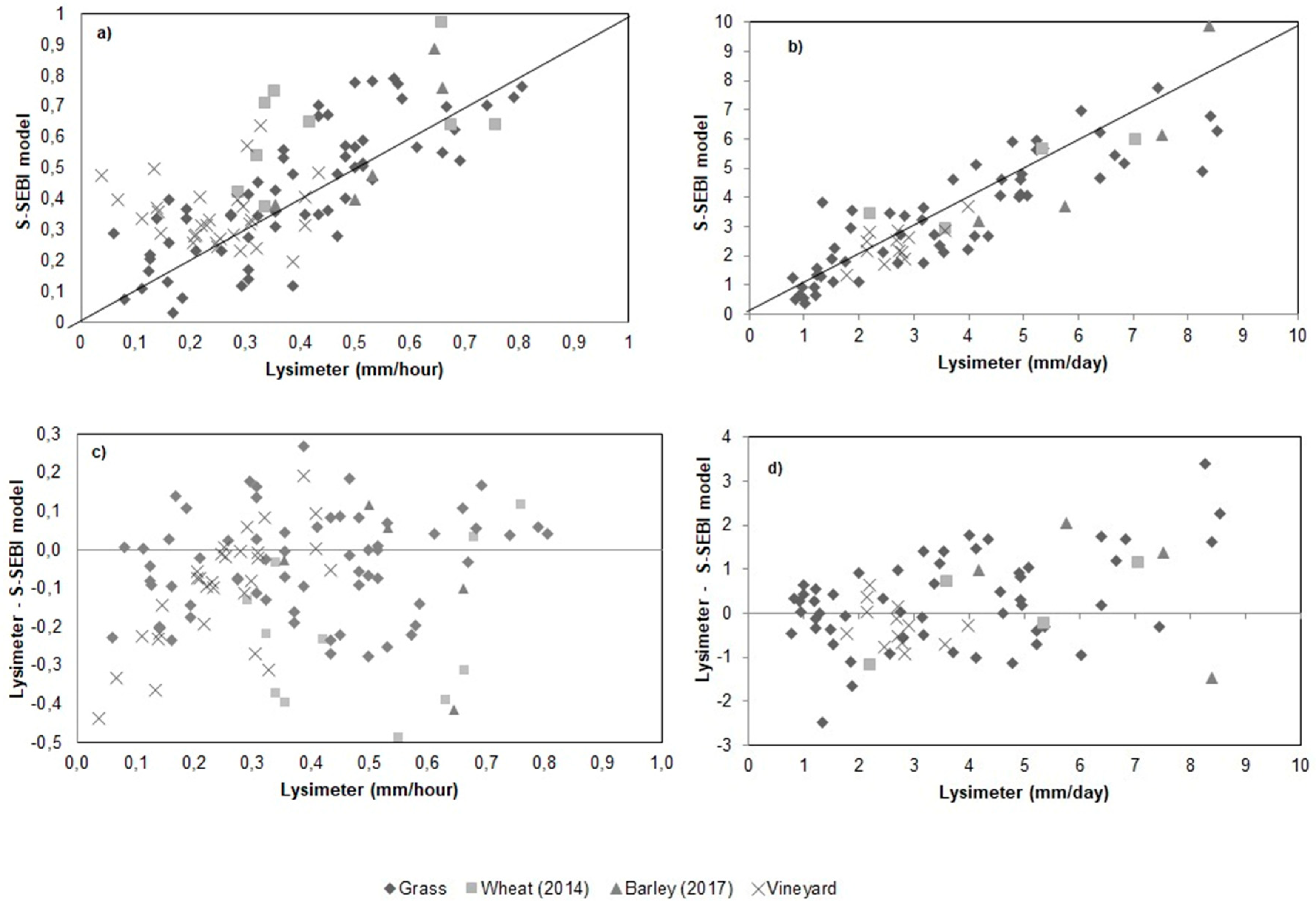
3.1. Comparison of S-SEBI Estimated and Measured ET

The comparison of the S-SEBI hourly and daily ET against lysimeter data for each land cover type is shown in Figure 3a,b, respectively. Generally, the daily estimates had moderately superior performance relative to the hourly estimates in all the land covers assessed. Grass produced the best linear relationship with the in situ ET data. This may indicate that the relation is better when the land cover is more homogeneous. The biases of the hourly and daily ET estimated by the S-SEBI in comparison to the lysimeter data were also plotted and are exhibited in Figure 3c, d. When the bias is positive, the model overestimates the ET, which was observed mostly for dates with low values of ET. The hourly bias of the S-SEBI varied between -0.4 mm/h and 0.4 mm/h (Figure 3c), and the ET overestimation of the in situ values occurred essentially between 0.05 mm/h and 0.6 mm/h. On the other hand, when the in situ ET is higher (between 0.6 mm/h and 0.9 mm/h), the model tends to underestimate the ET. A similar random pattern was seen in the daily bias, which varied between −3.2 mm/day and 5.3 mm/day, producing values closer to zero (Figure 3d).

A difference of 12% (0.45 mm/day) was found between the S-SEBI model and the lysimeters, with an average daily ET for all the land covers of 3.55 mm/day and 4.01 mm/day, respectively. In contrast, the average hourly ET is 0.44 mm/h for the S-SEBI and 0.36 mm/h for the lysimeters, with a difference of 15% (−0.07mm/h). Different accuracy situations have been reported in the literature for remote sensing-based ET models in comparison to lysimeter data. Using the METRIC model, Chavez et al. [41] found similar but slightly larger errors for hourly ET in comparison to the daily values. An evaluation carried out in Tanjung Karang, China, used the SEBAL model and meteorological and lysimeter data over cultivated rice and found that the determination of ET by satellite data overestimates the values obtained from lysimeters by 10% [42]. In a semiarid climate in Las Tiesas, Spain, different models overestimated the lysimeter measurements between 3% and 70% depending on the method applied [43]. Mkhwanazi et al. [44] developed a modified SEBAL model that requires daily averages of limited weather data and validated it against lysimeter data over an Alfalfa field. The authors reported average underestimates with values up to 24% for the modified model and up to 38% for the original SEBAL algorithm.

Table 3. Statistical analyses of the S-SEBI model performance with daily (mm/day) and hourly (mm/h) lysimetric data.

	Grass		Wheat (2014)		Barley (2016)		Vineyard
	Hour	Daily	Hour	Daily	Hour	Daily	Hour	Daily
Bias a	−0.04	0.52	−0.10	−0.50	0.08	1.24	−0.00	−0.43
MSD b	±0.09	±0.98	±0.16	±1.45	±0.09	±1.18	±0.09	±0.46
RMSE c	0.10	1.11	0.19	1.53	0.16	1.71	0.09	0.63

^a Bias = Σ (Oi − Pi)/n; where O_i is the observed ET, and P_i is the ET modeled. ^b Mean standard deviation. ^c Root mean square error.

summarizes the statistical metrics of the hourly and daily ET between the S-SEBI and lysimeter data. Good agreements were obtained from the satellite-based estimates, with RMSE varying from 0.1 mm/h to 0.19 mm/h for hourly and from 0.63 to 1.71 for daily ET, respectively. These results are in accordance with other validation exercises reported for the S-SEBI model worldwide [4,6,20,22,23,31,45].

The performance of the hourly ET produced superior estimates for Grass and Vineyard, with an RMSE and MSD of 0.10 and ±0.09 for Grass and 0.09 and ±0.09 for Vineyard, respectively. Wheat and Barley had the worst hourly ET estimates, with an RMSE and MSD of 0.19 and ±0.16 for Wheat and 0.16 and ±0.09 for Barley, respectively. Knowledge of the hourly ET has several advantages, and its accuracy evaluation plays an important role in quantifying estimation errors with irrigation water management practices. However, the hourly satellite calibration is a typical source of uncertainty in satellite SEB models. Hashem et al. [46] compared the hourly ET with lysimeter data in Texas. By using the METRIC model, the authors found average RMSEs of 0.14 mm/h and 0.16 mm/h for dry and irrigated agriculture lands, respectively. Despite the fact that the METRIC model was developed with a focus on agriculture areas and is proven to perform very well for these land covers, its computation requires one to determine roughness length, which is a complicated variable to retrieve with enough accuracy from classic remote sensing methods [17]. Moreover, over crops in Texas, Gowda et al. [27] compared the performance of the hourly ET from the SEBS model with data from four lysimeters using a dataset of 16 Landsat 5 images. The authors reported high accuracy with an average RMSE of 0.11 mm/h. Nevertheless, they pointed out that a locally derived surface albedo-based G model improved the G component estimates. The limitations of the empirical formulation used to derive G from remote sensing have already been emphasized in other works [23,24]. Furthermore, roughness length is also required in SEBS model computation, in addition to other meteorological inputs, such as air temperature, humidity, and wind speed measured at a reference height, which sustains the superiority hypothesis of the S-SEBI in terms of simplicity. The hourly biases of the land covers assessed were mostly negative except for Barley, which produced 0.08. This indicates that the hourly ET was predominantly underestimated.

The performance of the daily ET estimates, such as the hourly estimates, produced the best metrics for Grass and Vineyard, with an RMSE and MSD of 1.11 and ±0.98 for Grass and ±0.46 and 0.63 for Vineyard, respectively. The daily bias exhibited negative results for Wheat and Vineyard, with values of -0.50 and -0.43, respectively. Unlike the hourly metrics, the daily ET results of Wheat are notably better in comparison to Barley. However, it is worth mentioning that the amount of available data for Barley is reduced relative to the other land cover types, and, consequently, it may not have properly included the annual and pluriannual variability of ET. In order to evaluate the influence of weather conditions (particularly cloud cover impacts) on the S-SEBI model’s accuracy, we calculated the statistical metrics and excluded the days with clouds, which are discussed in the next section.

3.2. Uncertainties in the S-SEBI Estimates

The concept of evaporative fraction is the basis of the S-SEBI model. However, its diurnal constancy may not be satisfied under cloudy circumstances [47]. Therefore, we selected 55 entirely cloud-free scenes to evaluate the performance of the algorithm under ideal conditions.

Table 4. Statistical analyses of the S-SEBI model performance with daily (mm/day) lysimetric data, excluding partial cloudy days (n = 55).

	Grass	Wheat (2014)	Barley (2016)	Vineyard
Bias	0.28	0.09	0.73	−0.27
MSD	±0.80	±0.8	±1.10	±0.37
RMSE	0.85	0.81	1.32	0.46

shows the statistical metrics obtained in the daily analysis. The results found demonstrate a considerable improvement in the ET estimates when the atmospheric conditions do not vary much during the day. In general, the average RMSE decreases from 1.25 mm/day to 0.86 mm/day when only ideal scenes are used. The low errors suggest that the model works very well for the estimation of ET in all the land covers. The RMSE was found to be 0.85 mm/day for Grass, 0.81 mm/day for Wheat, 1.32 mm/day for Barley, and 0.46 mm/day for Vineyard. The MSD indicates that the differences between model results and lysimeter data are less than 1 mm/day, which is in agreement with Sobrino et al. [31].

Typically, in the S-SEBI model, errors in the determination of TH and TLET lines (and consequently in the evaporative fraction) impact the obtention of the instantaneous LET, which directly affects the ET estimates. Afterward, the daily ET is extrapolated from instantaneous to daily ET by using the C_di (Equation (6)). According to Singh and Senay [48], different methods of upscaling have their own bias. Yang et al. [49] demonstrated that in most of their dataset, variation of the evaporative fraction during daylight tended to be stable within the time window of 10:00 and 15:00 UTC. However, after this window, it is not constant and can affect the C_di. According to some authors [14,50], there are many difficulties to convert instantaneous ET into daily ET, mostly due to the non-stable conditions of the evaporative fraction during a daylight period, which vary with the available energy, surface resistance, and other environmental variables. However, because in the S-SEBI model the daily ET is calculated using the available net flux radiation during the day, the daily ET estimates produced are reliable [21,31], which can be considered a strength of the methodology applied. 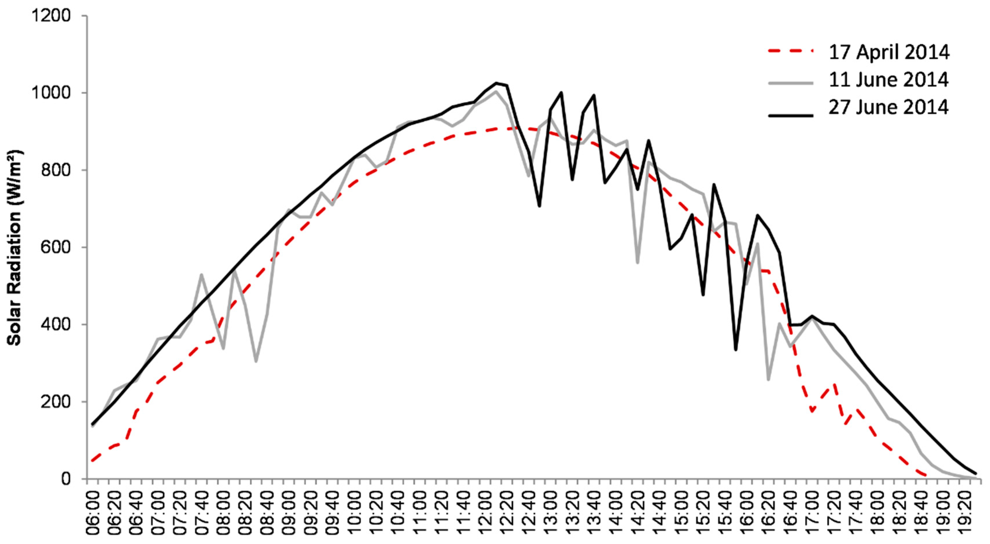Figure 4 illustrates the behavior of the solar radiation during different DOYs. The solar radiation data from the flux tower were analyzed on the DOY of greatest errors (11 June 2014—DOY 162 and 27 June 2014—DOY 178) and compared with a DOY with good linear relationship (17 April 2014—DOY 107).

The “noises” observed in the solar radiation curve clearly reflect the differences between the observed and estimated daily ET. In a clear-sky day when the solar radiation does not show noises caused by clouds or large amounts of water vapor, the S-SEBI-based estimates exhibit an accuracy much lower than 1 mm/day. On 17 April 2014 (DOY 107), the difference between the in situ ET and calculated ET is 0.23 mm/day. In contrast, when the daily solar radiation curve presents some noises and the weather conditions vary widely during the day, the difference between the in situ ET and the model estimates is 2.92 mm/day for 6 November, 2014 (DOY 162), and 1.89 mm/day for 27 November 2014 (DOY 178). In addition to the solar radiation, seasonal drivers from the land surface can strongly affect the ET, making the estimates differ substantially. Yang et al. [49] examined remote sensing-based ET estimates from high-resolution data over Wheat in different months and reported an overall RMSE of 0.67 mm/day. The authors pointed out that in months with low coverage and row pattern at the turning green stage, the satellite-based ET accuracy is impacted. In contrast, when the crop is at the harvest stage, better estimates are produced. This occurs particularly because at the time that the normal crop physiological and ecological processes are gradually ending, the soil evaporation is over again, the main contributor to ET.

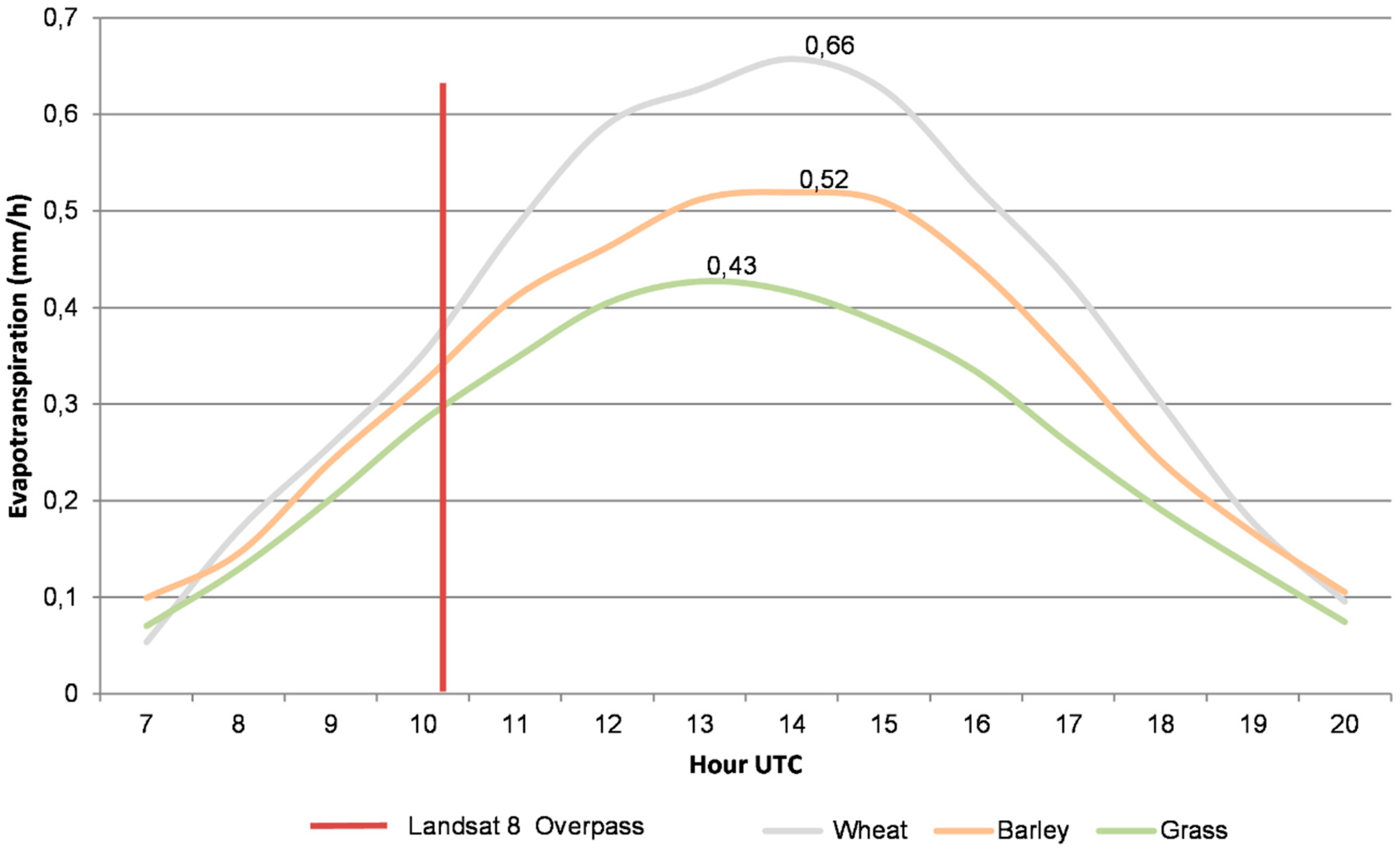
3.3. Variation of ET during the Daytime

At the Barrax site, the lysimeters are located in the center of 100 × 100 m plots, and the data are available hourly. As some in situ ET data were missing for Vineyard, they were not included. The average daily ET measured for the entire period was 5.4 mm/day for Wheat, 4.6 mm/day for Barley, and 3.7 mm/day for Grass. Given that differences in the thermal, wind, and weather conditions and the radiation regime between a lysimeter device and its surroundings can affect the measurements [51], we investigated the hourly average for each land cover type. Figure 5 displays the hourly averages of ET and the maximum values obtained from the lysimeters.

Overall, the ET exhibits typical fluctuations in shape during the day, varying between 7:00 and 20:00 UTC. The hourly ET for Grass ranged from 0.03 mm/h to 0.43 mm/h, with an hourly average of 0.24 mm/h and its maximum value at 13:00 UTC. For Wheat, the hourly ET ranged from 0.04 mm/h to 0.66 mm/h, with an hourly average of 0.36 mm/h and its maximum value at 14:00 UTC. Finally, for Barley, the hourly ET ranged from 0.05 mm/h to 0.52 mm/h, with an hourly average of 0.30 mm/h and its maximum value at 14:00 UTC. Yang et al. [52] reported noticeable daytime ET variations between 7:00 and 18:00, with a peak typically occurring at approximately 14:00 UTC.

Although between 13:00 and 15:00 UTC the ET measurements for each land cover are relatively constant, the maximum differences between curves are more significant in this period. However, at the time of the Landsat 8 overpass (10:42 UTC), the in situ ET values increased notably quicker. This behavior was observed for all the land cover types. In the S-SEBI model application, the conversion from instantaneous to daily ET through the C_di assumes that at the time of the satellite overpass, the highest value of ET is being measured; nevertheless, the maximum ET values are seen after the Landsat 8 overpass, around 13:00–14:00 UTC. Consequently, the discrepancy between the hourly ET in situ and the instantaneous ET from Landsat 8 can be a potential source of uncertainty for ET validation.

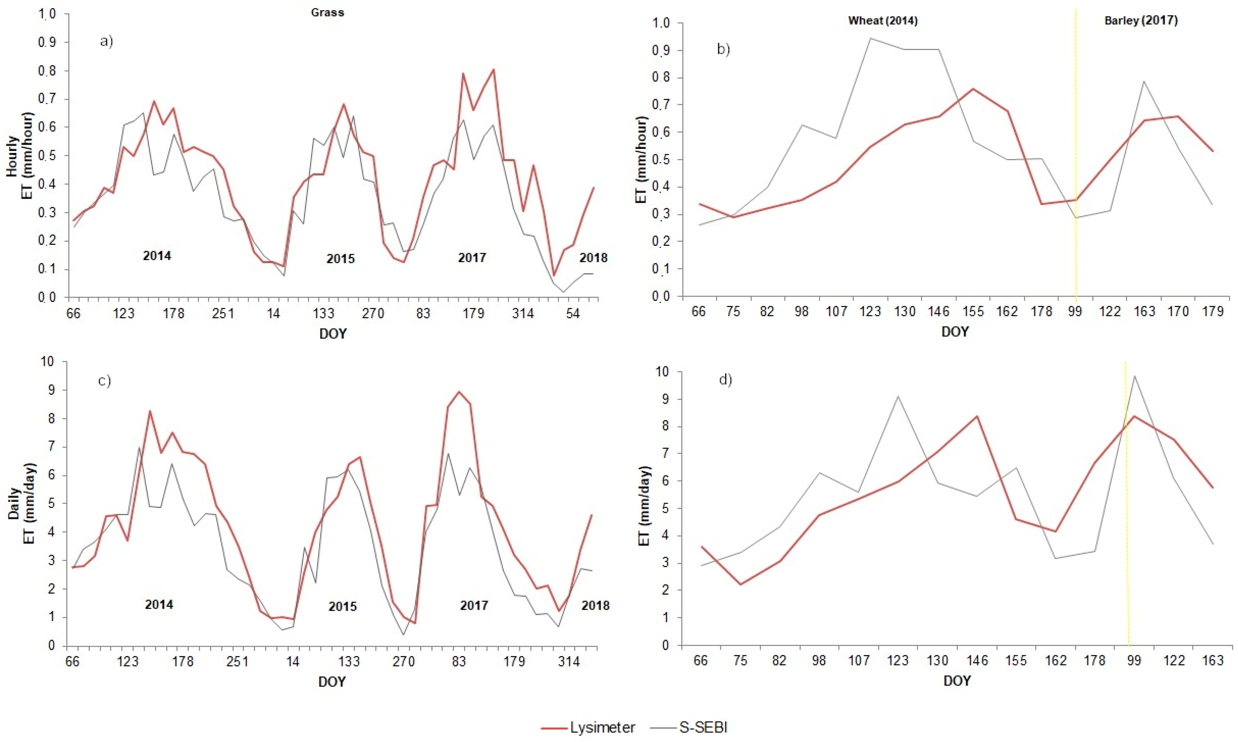
3.4. Seasonally Distributed ET

Figure 6 shows the distribution of the hourly and daily ET from the S-SEBI compared to lysimeter ET in situ values for the whole period. Similar patterns were found in daily ET for Grass, Wheat, and Barley fields between seasons, which demonstrates a clear seasonal pattern, with higher values in summer and lower values in winter due to the cold weather conditions [53]. Figure 6a,c illustrate the hourly and daily ET in the Grass field, respectively. The hourly ET ranged between 0.06 mm/h during the winter season and 0.8 mm/h in summer and spring seasons. In most cases, the modeled ET underestimates the values measured by the lysimeter, as while the average lysimeter ET is 0.39 mm/h, the predicted is 0.34 mm/h. The largest differences between predicted and observed daily ET were noted also in the summer season (DOY 170/2017), in which the lysimeter ET was 8.94 mm/day and the predicted ET was 5.3 mm/day. These results are in agreement with López-Urrea et al. [43], where FAO Penman–Monteith was applied and compared with lysimeter data. The authors pointed out that the model underestimated ET values mainly during periods of greater evaporative demand.

In Figure 6b,d, we depict the hourly and daily ET results in the Wheat and Barley fields. When the satellite-based hourly ET exceeds the lysimeters’ observations, the daily ET tends to exhibit the same behavior. As a crop field is irrigated according to its water need to prevent stress, the only important factor that affects the ET results is the growing and harvesting season. As it was pointed at the end of Section 3.2, when low crop coverage is present (DOYs 82–123), the model shows more uncertainties in comparison to the late stages of the crop. The S-SEBI model also outperforms when very high and low ET values are achieved. This overtaking was already reported in other studies for the S-SEBI model. Käfer et al. [23] compared ET estimates derived from the S-SEBI with a neural network-based model in Southern Brazil, which suggested that the S-SEBI values tend to decrease accuracy in estimating extreme ET values, commonly in the transition seasons between winter and summer.

The overestimates from the S-SEBI model, which were more pronounced in the summer–spring season, were already reported [12]. The authors claimed that, particularly during severe drought conditions, the parameterization will overestimate ET. The biggest difference between hourly ET occurred in the spring season (DOY 123/2014), in which the standard deviation was 0.39 mm/h and the highest rate of water loss occurred. These findings are in accordance with Liu et al. [53], who observed the highest ET in May after the over-wintering period. The differences between estimated ET and lysimeter data can be explained by the evaporative fraction calculation in the S-SEBI model. Summarily, on DOY 123, for higher albedo values, the Ts does not increase significantly as expected; consequently, it generates a greater error in the Ts determination to dry and wet conditions. On DOY 163/2017 over the Barley field, a similar behavior was seen. This evidences the limitation of the S-SEBI model when operationally applied. The relationship between higher albedos and Ts is well documented in the literature. Sobrino et al. [31] and Gómez et al. [17] demonstrated that identifying the boundary limits to obtain the evaporative fraction is the critical point of this method and reported that in some cases it reached 1.4 mm/day. In addition, differences between in situ and estimated ET can be related to the extension of the area evaluated, especially given the contrast influence in the landscape that may result in pixel mixing in the albedo and Ts determination. The fact that the cultivated area is smaller than the 30 meter pixel size presents scale issue to the Ts estimated and, therefore, the validation results. In this study, although we used a fixed percentile value for the whole dataset, the ET estimates produced a very high accuracy, and the cloudy effect clearly compromises the albedo–Ts relationship more significantly than the other factors mentioned.

3.5. Spatially Distributed ET

Remote sensing techniques have provided an efficient way to retrieve multi-year, spatially consistent, and temporally continuous ET products on the regional to global scale [5,23,25,31,54]. One of their main advantages is to provide estimates from the whole territory, capturing small spatial variations between pixels that allows one to assess the efficiency of the water use and irrigation and groundwater recharge projects or return flows [41]. 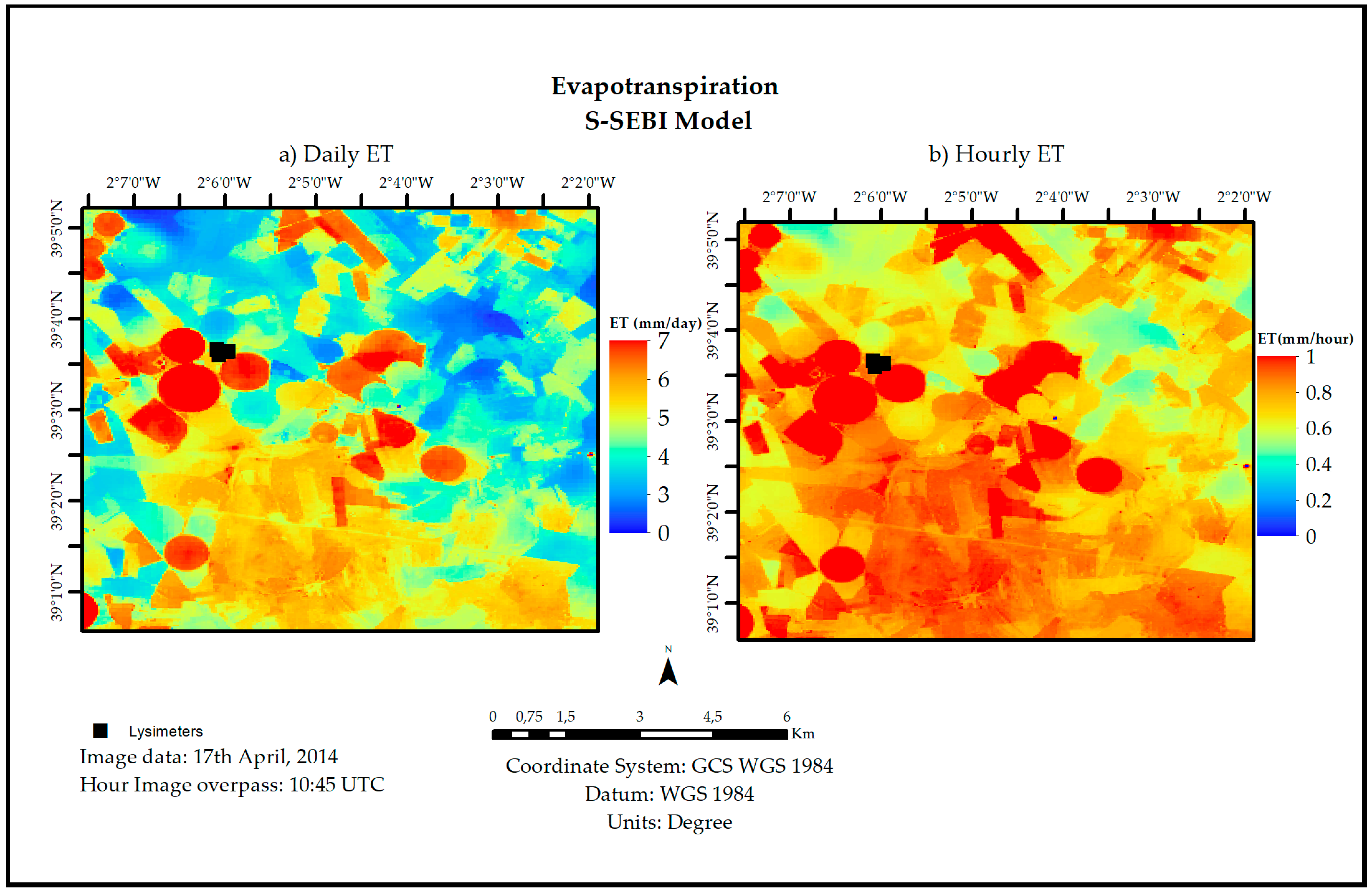Figure 7 exhibits the spatial pattern of daily and hourly ET obtained from the S-SEBI method by using a Landsat 8 image over Barrax in the spring season, 17 April 2014 (DOY 107). Overall, the S-SEBI model can capture the spatial variability of evaporative demand of the atmosphere over the whole study area. Specifically in the daily ET map (Figure 7a), the bare areas with lower ET (blue color) and crop areas with higher ET (red color) can be well distinguished. There were no differences between in situ measurements (lysimeter data) and from the S-SEBI model in Grass land cover. In contrast, over the Wheat field, a difference of 0.24 mm/day was found. In the hourly ET map (Figure 7b), the bare areas with lower ET are less prominent and discriminated from the other fields and irrigated areas. The hourly ET average was 0.6 mm/h, which is close to the hourly average ET of April (0.64 mm/h). The difference between in situ data and the S-SEBI model was 0.16 mm/h in Grass and 0.23 mm/h in the Wheat area.

In addition to the smaller error obtained in the daily analysis discussed in Section 3.2, spatially, the daily analysis has more contrast in areas with higher ET and potential water deficit. These findings are important with regard to the water planning of agricultural areas, considering that effective water resource management requires an accurate estimation of the water use and availability to face challenges of water scarcity [55].

4. Conclusions

The ET is a key component of water balance, and despite the significant advances in the last decades, remote sensing-based models are not free from uncertainties, especially when applied over different conditions for which they have not been originally developed or calibrated for. Therefore, assessing efficiency in techniques for monitoring water use is a constant research topic. In this paper, we investigated the ET obtained operationally by the S-SEBI model from Landsat 8 data between 2014 and 2018 at the Barrax Site, Spain. Four different land cover types were evaluated (Grass, Wheat, Barley, and Vineyard) and validated against lysimeter observations.

In general, the daily estimates produced slightly superior performance relative to the hourly estimates in all the land covers, with an average difference of 12% and 15% for daily and hourly ET estimates, respectively. Grass and Vineyard showed the best performance, with an RMSE of 0.10 mm/h and 0.09 mm/h and 1.11 mm/day and 0.63 mm/day, respectively. Nonetheless, when only ideal scenes (without any cloud cover) are considered, the accuracy expressly improves, indicating that the model works very well for all the land covers in suitable conditions. Thus, the S-SEBI model is able to retrieve ET from Landsat 8 data with an average RMSE for daily ET of 0.86 mm/day.

In the operational application of the S-SEBI, identifying operationally the boundary limits of percentiles to obtain the evaporative fraction is challenging. Our findings have shown that assuming a fixed percentile value (0.1%) for different crops can produce enough ET accuracy. In addition, although the conversion from instantaneous to daily ET is frequently cited as a limitation of the remote sensing-based ET models, the mechanism used to extrapolate instantaneous ET to daily values resulted in improved ET estimates; therefore, we strongly encourage the application of the C_di concept. In fact, the high accuracy of the in situ flux data used contributed to the good performance of the daily estimates. However, it is important to highlight that this is not a restriction, because hourly radiation data are available for the whole globe and can be easily obtained from several reanalysis products and used to generate trustable and continuous daily ET series [56].

The hourly ET obtained from the lysimeters provided a detailed analysis of the ET pattern during the day. Between 13:00 and 15:00 UTC, the ET measurements for all the land covers are relatively constant, and the maximum values occurred at 13:00–14:00 UTC. At the time of the Landsat 8 overpass (10:42 UTC), the in situ ET values showed a rapid increase. Because the C_di assumes that at the time of the satellite overpass the highest value of ET is being measured, which it clearly is not, the discrepancy between the hourly ET in situ and the instantaneous ET from Landsat 8 can be a source of uncertainty. The overpass of the Landsat missions represents neither the maximum daily ET nor the average daily ET. Differently, more significant variations are seen 10:00–11:00 UTC, which contribute to increase errors in the estimated ET. In addition, it is worth mentioning that the Landsat pixel size also does not appropriately represent the test sites to validate ET; i.e., the spatial resolution of the TIR sensor of the Landsat satellite is not fully adequate for ET estimates. However, it is expected that with the new Sentinel projects and the improved resolution, these issues will be minimized.

The S-SEBI is a model of simple application and low dependence of complex inputs that can well capture the spatial variability of evaporative demand and produce robust daily ET maps over different crops without much effort. Hence, it can be used to operationally retrieve ET from agriculture sites with good accuracy and sufficient variation between pixels, thus being a suitable option to be adopted into operational ET remote sensing programs for irrigation scheduling or other purposes.