Sub-Decimeter Onboard Orbit Determination of LEO Satellites Using SSR Corrections: A Galileo-Based Case Study for the Sentinel-6A Satellite

Abstract

In GNSS-based navigation onboard Low Earth Orbit (LEO) satellites, typical accuracy requirements are 10 cm and 0.1 mm/s for 3D position and velocity, respectively. Previous works have shown that such performance is achieved by including Galileo measurements in the estimation process. Here, we aim to evaluate the impact of employing State Space Representation (SSR) corrections, i.e., GNSS satellite orbit, clock, and biases, to be applied to the broadcast ephemerides. In this framework, the Precise Onboard Orbit Determination (P2OD) software (SW) tool developed at the University of Padua (UNIPD) is used to investigate the needs of onboard navigation. The UNIPD SW employs an Extended Kalman Filter (EKF) using a reduced-dynamics approach. The force model implemented is adapted to onboard processing, and empirical accelerations are included to take into account residual force mismodeling. Actual observation data from the LEO Sentinel-6A satellite are processed along with SSR corrections from the CNES service. Galileo-based solutions are compared to ground-based POD reference orbits. The analysis suggests that the use of SSR corrections provides sub-decimeter and below 0.1 mm/s accuracies in 3D position and velocity, respectively. Such results indicate a P2OD solution quality close to that achievable by adopting precise orbits and clocks.

1. Introduction

Recently, the growing number of Low Earth Orbit (LEO) constellations has become a hot topic in the scientific and technological communities. Multiple applications are envisioned for these constellations. One of the main usages concerns augmented signal coverage over Earth. The idea is to extend the worldwide availability of services such as internet connections and GNSS-based positioning. Regarding the LEO-enhanced system for positioning relying on GNSS signals, accurate knowledge of LEO satellite orbits is required [1]. Specifically, LEO constellation signals can be exploited to improve the GNSS-based Precise Point Positioning (PPP) in terms of convergence time and performance in harsh scenarios [2]. Similar to the necessity of employing precise GNSS orbits and clocks, such needs increase the interest in having precise LEO orbits in real-time and, therefore, Precise Onboard Orbit Determination (P2OD).

The Sentinel-6A (S6A) spacecraft is the first launched vehicle of the Sentinel-6 mission, which aims to ensure continuity of service for sea surface altimetry based on the legacy of the TOPEX/Poseidon and Jason-1/-2/-3 missions [3,4]. The S6A satellite has a nominal altitude of 1336 km on a LEO orbit of 66${}^{\circ }$ with ground-track repetition after roughly 10 days. In the context of orbit determination, the spacecraft carries a redundant pair of PODRIX multi-frequency GNSS receivers, including Galileo signals. Previous authors have shown that the availability of Galileo measurements onboard enables a new level of accuracy for real-time orbit determination. Galileo-based decimeter-level onboard orbital positioning using broadcast ephemerides has been presented in [5] and the decimeter-level is reported in [6]. Although the quality of broadcast GNSS ephemerides is improving in general [7], such performance is achieved mostly because of the high quality of the Galileo navigation data. The latter benefits from more-stable hydrogen maser clocks and a more-frequent refresh rate (once every 10–30 min) of their broadcast ephemerides compared to GPS. The higher quality of broadcast ephemerides affects the observation model by decreasing the level of orbit and clock errors down to less than 20 cm [8]. As a consequence, navigation messages can be applied for carrier-phase-based positioning techniques [9].

The current real-time onboard scenario is expected to be possibly further improved once the Galileo High Accuracy Service (HAS) is fully functional and capable of providing State Space Representation (SSR) corrections at the same level as those generated with a dense global network of reference stations. In this way, the GNSS orbit and clock errors impacting the observation model are lowered to a level close to precise orbit and clock products. Recently, the European Union published the Galileo HAS signal-in-space interface control document (HAS SIS ICD) [10], which describes the encoding, decoding and application of the messages. An assessment on the P2OD impact of using the current status of such corrections has been addressed in [11]. In their work, the authors processed HAS data collected during an early test campaign in September 2021 and assessed its benefit for (near) real-time orbit determination of the Sentinel-6A satellite (S6A). The corrections they used represent the pre-operational performance of the Galileo HAS service. The authors showed that the 3D orbit estimation is improved by using the broadcast GNSS ephemerides corrected by the HAS messages. In particular, the 3D RMS error of GPS-only processing improves by 40–50%, while the performance gain when also using Galileo amounts to roughly 10%. This result is due to the already high quality of the Galileo broadcast ephemerides.

The HAS corrections are thought to be applied similarly to the standardized format of the Radio Technical Commission for Maritime Services (RTCM) [12]. GPS-based real-time Precise Orbit Determination (POD) using RTCM-SSR orbit and clock corrections from the Centre National D’Etudes Spatiales (CNES) has been assessed in [13]. In their work, the authors show that sub-decimeter positioning is feasible when correcting the broadcast ephemerides with orbit and clock SSR corrections from the CNES CLK93 mountpoint and without Integer Ambiguity Resolution (IAR).

Here, we aim to evaluate the quality of the Galileo-based estimated S6A dynamical state vector when correcting the broadcast ephemerides. The work is a continuation of the study carried out in [6]. In particular, the main topics that we address are the following: First, we aim to understand which level of onboard POD performance can be foreseen once the HAS corrections have the same accuracy as the CNES RTCM-SSR corrections. Second, we show a strategy to successfully handle data correction outages and potential phase bias jumps from the perspective of performing IAR. Third, the quality of the estimated solution obtained by using a Galileo-only configuration is assessed. The computation is based on software (SW) developed at the University of Padua (UNIPD), which was first presented in [14], and will be part of the upcoming ESA/GOMspace GOMX-5 in-orbit demonstration CubeSat mission [15] within the Deimos G3PSTAR GNSS receiver [16].

The paper is organized as follows: After introducing the measurement dataset together with the ancillary and SSR correction data, the algorithms and models employed in simulated real-time processing are presented. Subsequently, we discuss and compare the results achieved by adopting RTCM-SSR corrections to those obtained by using the broadcast ephemerides only. Finally, the main conclusions are summarized, and an outlook on future work is provided.

2. The Dataset

GPS and Galileo S6A measurements are processed.

Table 1. Dataset processed in this work, including satellite data, measurements, GNSS ephemerides, and antenna and SSR corrections.

Item	Description
	Non-Sun-synchronous LEO orbit
	Repeat cycle: 9.92 days
S6A orbit	Mean altitude: 1336 km
	Eccentricity: 0.000094
	Inclination: 66${}^{\circ }$
S6A spacecraft	Mass: 1180.6 kg
parameters	CoM position: (1.533 m, −0.007 m, 0.037 m)
	First
	Start: 2021-09-04 00:00:00.0
Time intervals	End: 2021-09-04 18:36:30.0
(GPS time)	Second
	Start: 2021-09-24 00:00:00.0
	End: 2021-09-30 23:55:0.0
	RINEX GNSS navigation data
GNSS orbits and clocks	GPS: CNAV L1/L2 P(Y)
	Galileo: FNAV E1/E5a
SSR corrections	RTCM-SSR corrections from CNES mountpoint SSRA00CNE0. Update interval: 5 s
GNSS satellite code biases	TGD and ISC for L1 (1C) and L2 (2L) from GPS CNAV message
	GNSS transmitting satellite: not applicable, zero PCO and PCV
	S6A receiver:
GNSS antenna PCV	ARP (2.475 m, 0.000 m, −1.080 m)
	PCO + PCV from in-flight calibration
	PCO L1/L2 (0.00 mm, 0.00 mm, 73.00 mm)
	PCO E1/E5a (0.00 mm, 0.00 mm, 93.00 mm)
Earth Orientation Parameters	EOP IERS bulletin B
Solar Activity and Geomagnetic Activity	NOAA SAGA data

shows the dataset considered in the study, including satellite data [17], GNSS measurements, ephemerides, and antenna and SSR corrections, along with the necessary ancillary data. The S6A spacecraft is orbiting on an almost circular non-Sun-synchronous LEO trajectory at a mean altitude of 1336 km. RINEX-file-based GNSS pseudorange and carrier-phase observations at a 10 s sampling rate are processed during two independent time intervals in September 2021. Adopting the RINEX terminology [18], 1C/2L and 1C/5Q signals are utilized concerning GPS and Galileo, respectively.

For GPS, it has to be mentioned that, although 1W/2W measurements are available from the receiver, the current version of the UNIPD SW handles only one pair of signals per constellation. Therefore, the 1C/2L combination is preferred over the 1W/2W combination because of the higher availability of data.

Broadcast ephemerides from RINEX GNSS navigation data are used. While RINEX version 3.04 is considered for Galileo, the DLR RINEX version 4 [19] is adopted for GPS as it includes the CNAV navigation message that carries Time Group Delay (TGD) and Inter Signal Correction (ISC) information for 1C/2L signals. The broadcast navigation data are corrected by applying the RTCM-SSR corrections retrieved from the CNES mountpoint SSRA00CNE0 with an update interval of 5 s. Galileo orbit and clock corrections are no larger than 1 m in magnitude, while for GPS, they can reach 2–3 m. This behavior is aligned with the fact that the quality of the Galileo broadcast ephemerides is higher than that of GPS. Concerning the code biases, they are almost constant in the analyzed period, while variations of the phase biases of about a few centimeters, except for discontinuities, are observed. Since broadcast ephemerides are used, no GNSS Phase Center Offset (PCO) and Phase Center Variations (PCVs) are applied to the transmitting satellite antenna, while PCO and PCV are employed for the S6A receiver GNSS antenna. An ANTEX file provided by the European Space Agency (ESA) including L1/L2 and E1/E5a frequency values resulting from in-flight calibration is used, as described in [6].

The ancillary data comprise the Earth Orientation Parameters (EOP), i.e., the pole coordinates $xp$ and $yp$, the difference $\Delta$UT1 between Universal Time 1 (UT1) and Universal Time Coordinated (UTC), and Solar Activity and Geomagnetic Activity (SAGA) data. The former are retrieved from the IERS EOP Bulletin B in order to properly define the Earth-centered reference systems and their transformations. To model the atmospheric drag perturbation properly, the SW takes advantage of the SAGA data published by the National Oceanic and Atmospheric Administration (NOAA).

3. Algorithms and Models

The simulated real-time processing for orbit determination of the S6A satellite is based on an Extended Kalman Filter (EKF) algorithm. A reduced-dynamics approach [20,21,22] is employed to estimate the complete satellite dynamical state vector and to ensure the continuity of the solution through orbit propagation. Another advantage of adopting a reduced-dynamics approach is that it suffers less than the kinematic approach from poor constellation geometry [13,23].

Table 2. Force, observation, and estimation models employed in the orbit-determination process.

Item	Description
Force models
Earth gravity field	EIGEN-6c4, deg = 50, order = 50
Third-body perturbations	Point Mass model for Sun and Moon
Solid Earth tides	Compliant with IERS 2003
Relativity	Post-Newtonian corrections
Solar radiation pressure	Cannon-ball model, Conical Earth shadow
Atmospheric drag	Cannon-ball model, NRLMSISE-00 density model
Empirical accelerations	First-order Gauss–Markov process in RTN directions
Attitude	S6A nominal attitude model (with yaw-steering law)
Observation model
Measurement type	Ionosphere-free combination of dual-frequency pseudorange and carrier-phase GNSS observations
Phase wind-up	Corrected
Numerical integration	Runge–Kutta–Hull (2)4
Estimation
Type	Extended Kalman Filter
State parameters	position, velocity, drag, and SRP coefficients; empirical accelerations; receiver clock error; inter-system bias; carrier-phase ambiguities

summarizes the force and attitude models utilized in the dynamics model and the information concerning observation model, numerical integration, and estimation scheme employed in the filter.

3.1. Dynamical Model

The inertial Geocentric Celestial Reference Frame (GCRF) and the complete set of rotations between inertial, Earth-fixed and body-fixed frames are used to ensure the highest accuracy in the numerical integration of the spacecraft trajectory. Modeled in the GCRF, the equations of motion are

$${\displaystyle \frac{d\mathbf{r}}{dt}=\mathbf{v},\frac{d\mathbf{v}}{dt}=\mathbf{a},}$$

(1)

where $\mathbf{r}$ and $\mathbf{v}$ are the position and velocity of the satellite, respectively, and $\mathbf{a}$ is the total acceleration acting on the spacecraft. This acceleration can be expressed as follows

$${\displaystyle \mathbf{a}=-\mu \frac{\mathbf{r}}{r^3}+\mathbf{B},}$$

(2)

where $\mu$ is the Earth’s gravitational parameter, and $\mathbf{B}$ is the total sum of the disturbing accelerations. As reported in Table 2, the Earth gravity field EIGEN-6c4 [24] up to degree and order 50 is used with solid Earth tides (compliant with IERS 2003 [25], Luni–Solar third-body perturbations, and relativistic effects. The non-gravitational accelerations related to atmospheric drag and Solar Radiation Pressure (SRP) are included by adopting a cannon-ball spacecraft model. Finally, empirical accelerations are introduced in the modeling to compensate for residual force mismodeling [26]. These stochastic contributions along the Radial (R), transverse (T), and Normal (N) directions are treated as a first-order Gauss–Markov process with zero mean and correlation time set to 600 s. A Runge–Kutta–Hull (2)4 fixed-step method [27] is implemented for numerical integration of the satellite equations of motion. Such an integration method is used in the interest of onboard computational efficiency while ensuring adequate precision.

3.2. Observation Model

The Ionosphere-Free (IF) combination of pseudorange and carrier-phase observables are adopted in this analysis. The UNIPD SW processes dual-frequency measurements in either a single- or dual-constellation configuration. The IF observation model is the same as the one presented in [6]. Here, in addition, the observables are corrected by applying the RTCM-SSR corrections from the CNES mountpoint in accordance with [12]. In that case, the corrected IF pseudorange ($\tilde{p}$) and carrier-phase ($\tilde{\varphi }$) observations are modeled as

$$\begin{array}{cc}\hfill {\displaystyle \tilde{p}}& =\tilde{\rho }+c\left(d{t}_u-\widetilde{d{t}^s}+d{t}_{\mathrm{ISB}}\right)+ϵ\hfill \\ \hfill {\displaystyle \tilde{\varphi }}& =\tilde{\rho }+c\left(d{t}_u-\widetilde{d{t}^s}+d{t}_{\mathrm{ISB}}\right)+{\zeta }_u^s+A^s+\Psi +\eta ,\hfill \end{array}$$

(3)

where $\tilde{\rho }$ is the geometric distance between the GNSS satellite s at transmission time and the user receiver u at reception time considering the SSR-corrected GNSS satellite position, and c is the speed of light. Receiver and satellite clock offsets are identified by $d{t}_u$ and $\widetilde{d{t}^s}$, respectively. The satellite clock offset, $\widetilde{d{t}^s}$, includes the SSR clock corrections. An Inter System Bias (ISB) is included in case of a dual-constellation configuration and is set to zero for the reference constellation, i.e., GPS. Such a constellation-dependent bias comprises the system time difference, i.e., in this case, the GPS-Galileo Time Offset (GGTO) and all the receiver- and constellation-specific biases between the used and reference signals. As mentioned above, the pseudorange $\tilde{\rho }$ is corrected for the SSR code bias. In accordance with [12], the bias is applied to the uncombined observable for each satellite and signal. Similarly, the SSR phase bias is added to the uncombined carrier-phase observation. It is worth remarking that the phase bias correction is not required in this computation as no IAR is performed. However, it is included to verify that the filter strategy can handle such corrections in view of the adoption of an IAR algorithm. In addition, the receiver antenna PCV, ${\zeta }_u^s$, and an ambiguity term $A^s$ are added to the model. The phase wind-up effect $\Psi$ is corrected for in accordance with [28]. Regarding the S6A attitude, the nominal model with yaw-steering law is employed in accordance with the satellite specifications [17]. Finally, $ϵ$ and $\eta$ indicate the pseudorange and carrier-phase noise, respectively, including residual effects such as multipath.

3.3. Estimation

The EKF algorithm is self-initialized by a Single Point Positioning (SPP) solution generated using the first two epochs. The dimension of the EKF estimation state vector $Z^T$ varies between 12 + $n_A$ and 13 + $n_A$ for single- and dual-constellations, respectively. In the case with two constellations, in fact, the ISB is also estimated. Considering the number of ambiguities $n_A$, the estimation state vector can be written as

$${\displaystyle {\mathbf{Z}}^T=\left(\mathbf{r},\mathbf{v},C_D,C_R,a_R^e,a_T^e,a_N^e,d{t}_u,d{t}_{\mathrm{ISB}},A_1,\dots ,A_{n_A}\right).}$$

(4)

Along with the satellite dynamical state vector, the sequential filter estimates drag and SRP scaling parameters $C_D$ and $C_R$; the empirical accelerations in radial $a_R^e$, transverse $a_T^e$, and normal $a_N^e$ directions; the receiver clock error $d{t}_u$, the ISB $d{t}_{ISB}$, and the carrier phase ambiguities $A_1,\dots ,A_{n_A}$.

Furthermore, when using broadcast ephemerides without applying SSR corrections, the ambiguity term is modeled to absorb the effect of orbit and clock errors projected onto the line of sight by adopting process noise in the estimation, resulting in the so-called pseudo-ambiguity [29,30]. In that case, the standard deviation associated with the pseudo-ambiguity process noise is 0.1 mm and 0.8 mm for Galileo and GPS, respectively. Additionally, the empirical acceleration steady-state standard deviations result from a filter-tuning process. For both cases with and without SSR corrections, their values are 0.01 nm/s${}^2$, 0.01 nm/s${}^2$, and 0.12 nm/s${}^2$ in the radial, transverse, and normal directions, respectively.

Concerning the use of SSR corrections, it is necessary to smoothly handle the switch between applying or not applying corrections in order to avoid a sudden filter transient. The reason behind such an effect is that the corrected orbits and clocks define a precise reference system that is not maintained once the SSR stream stops. In other words, the amount of orbit and clock errors that affect the observation model abruptly change, and the filter has to adapt to the increased ephemeris error, resulting in a transient similar to the processing start. The strategy adopted to avoid this behavior is to re-initialize the ambiguities and their covariance so that the EKF algorithm is allowed to adhere to the new reference system. In addition to that, the pseudo-ambiguity process noise is adjusted accordingly. Ambiguity re-initialization is also used to handle phase bias jumps. A cycle slip is set every time there is a discontinuity in the phase bias for a specific satellite and signal. This discontinuity is identified by either an increased value of the Signal Discontinuity Counter of the RTCM-SSR phase bias [12] or by exceeding a threshold, which is empirically set to one meter.

The presented models and estimation strategy have been successfully tested in multiple configurations. It is worth mentioning that although the computation is performed offline, a true real-time scenario that operates continuously is reproduced. The results from using and not using the corrections are compared and presented in the following section.

4. Application of SSR Corrections: Orbit Determination Results

4.1. Methodology

The satellite dynamical state vector estimated using the UNIPD SW is evaluated with respect to orbits generated by on-ground batch processing. Publicly available orbits with a one-minute time step provided by the CNES-SSALTO/POD team are selected as the reference for the comparison [31]. These orbits are identified by the CNES-POD acronym hereafter. The 3D RMS of the CNES-POD orbits is about 2–3 cm as reported in the EUMETSAT Sentinel-6 A GNSS-RO NTC Cal/Val Report [32]. Single- and dual-constellation configurations are processed, i.e., using observations either from:

• Galileo only: hereafter named the E configuration;
• GPS and Galileo: hereafter named the GE configuration.

Moreover, the benefit from applying the RTCM-SSR corrections from the CNES mountpoint is assessed. The solution obtained by using the corrections is named RTCM, while the results without corrections are identified as BRDC.

As reported in Table 1, two independent time intervals are analyzed. The first one is a period of roughly 18 h of continuous corrections data in which the full potential of applying the corrections is evaluated in a dual-constellation configuration. On the other hand, during the second time interval of seven days, the continuity of the RTCM-SSR messages is not ensured. This scenario allows us to validate the estimation strategy that involves ambiguity re-initialization. Furthermore, in that case, the Galileo-only solution is investigated, addressing the third research topic of this work.

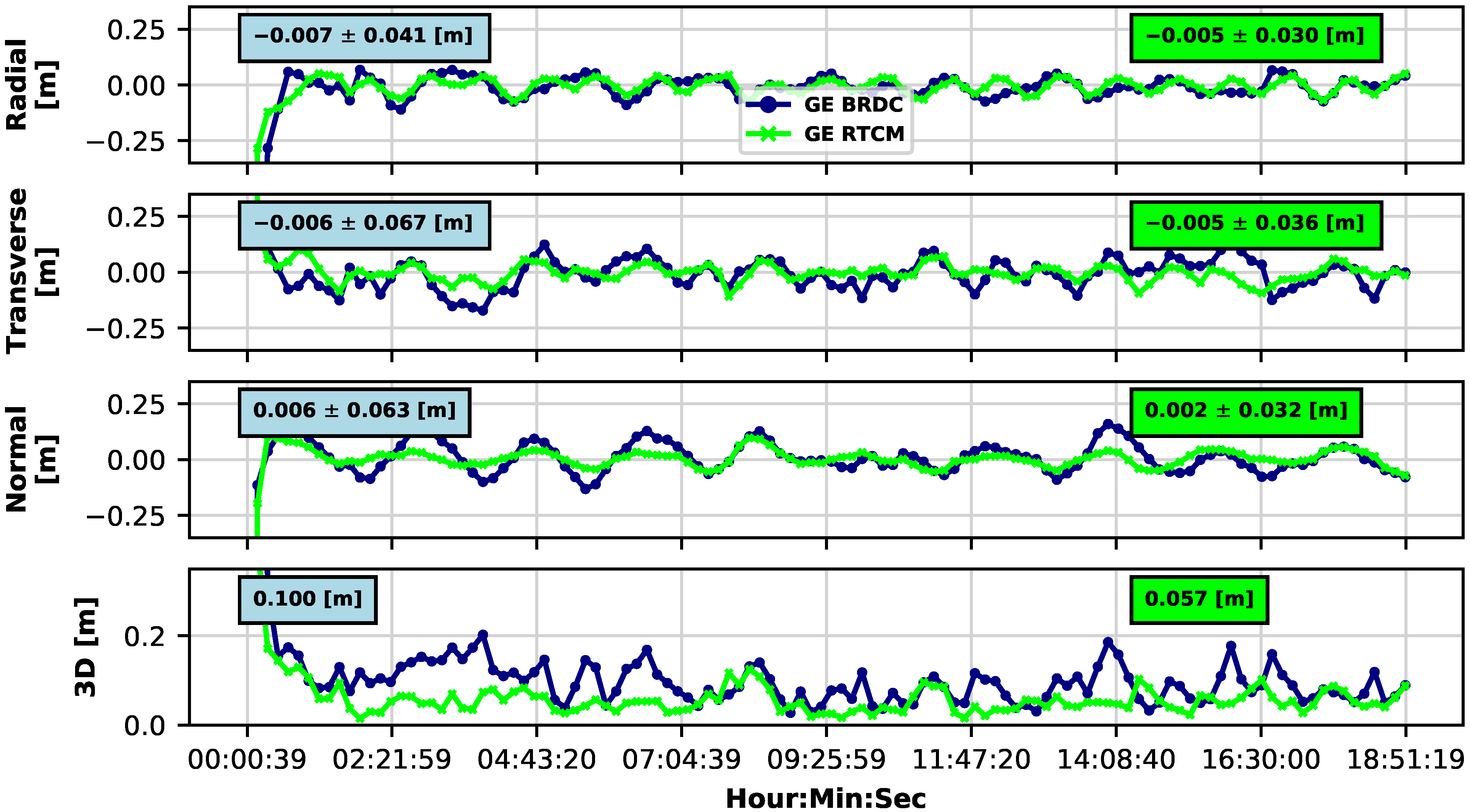
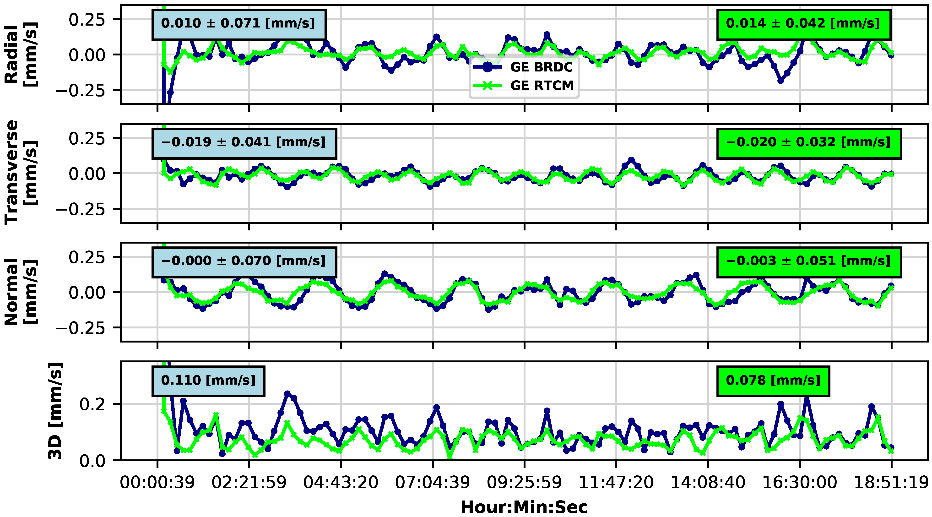
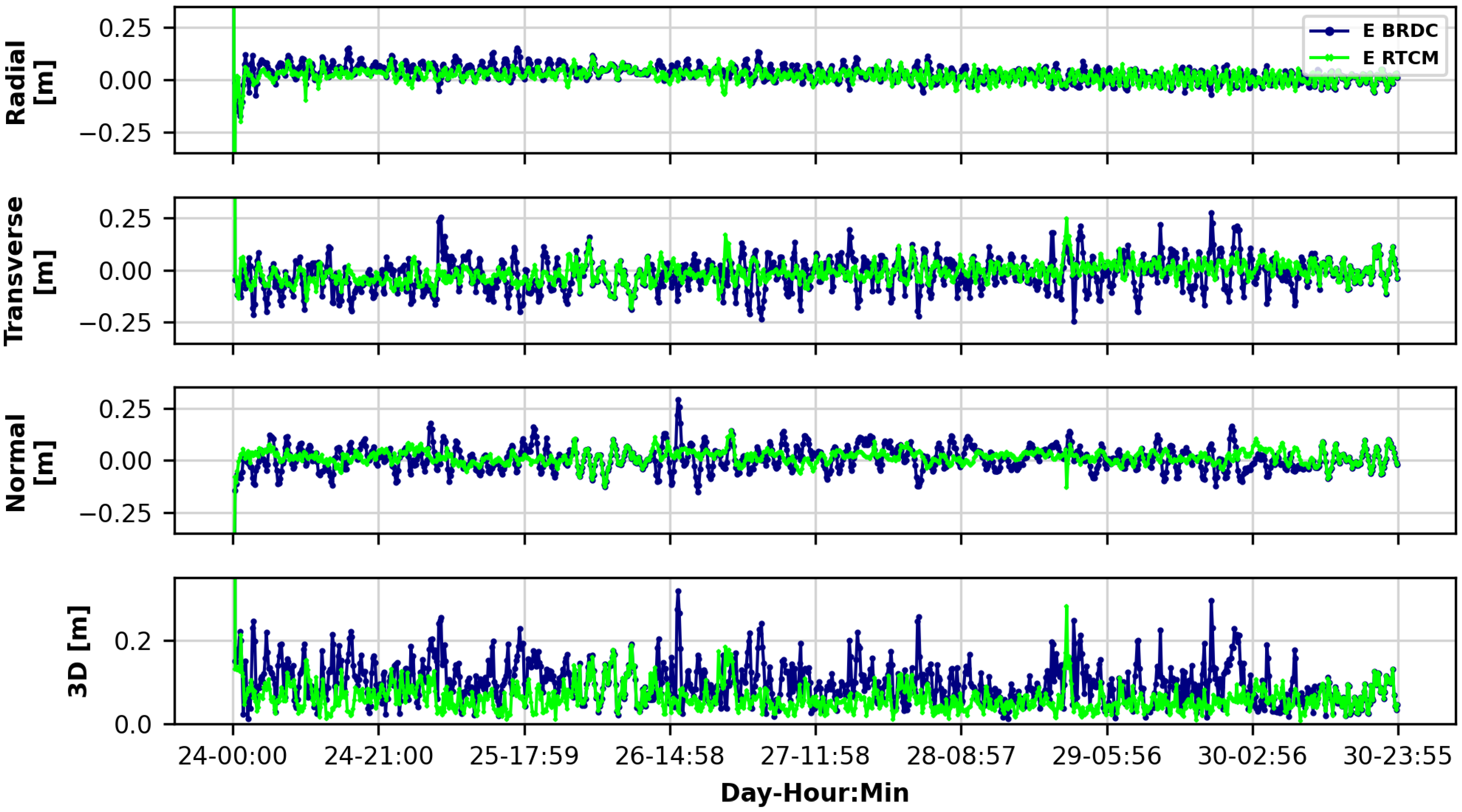
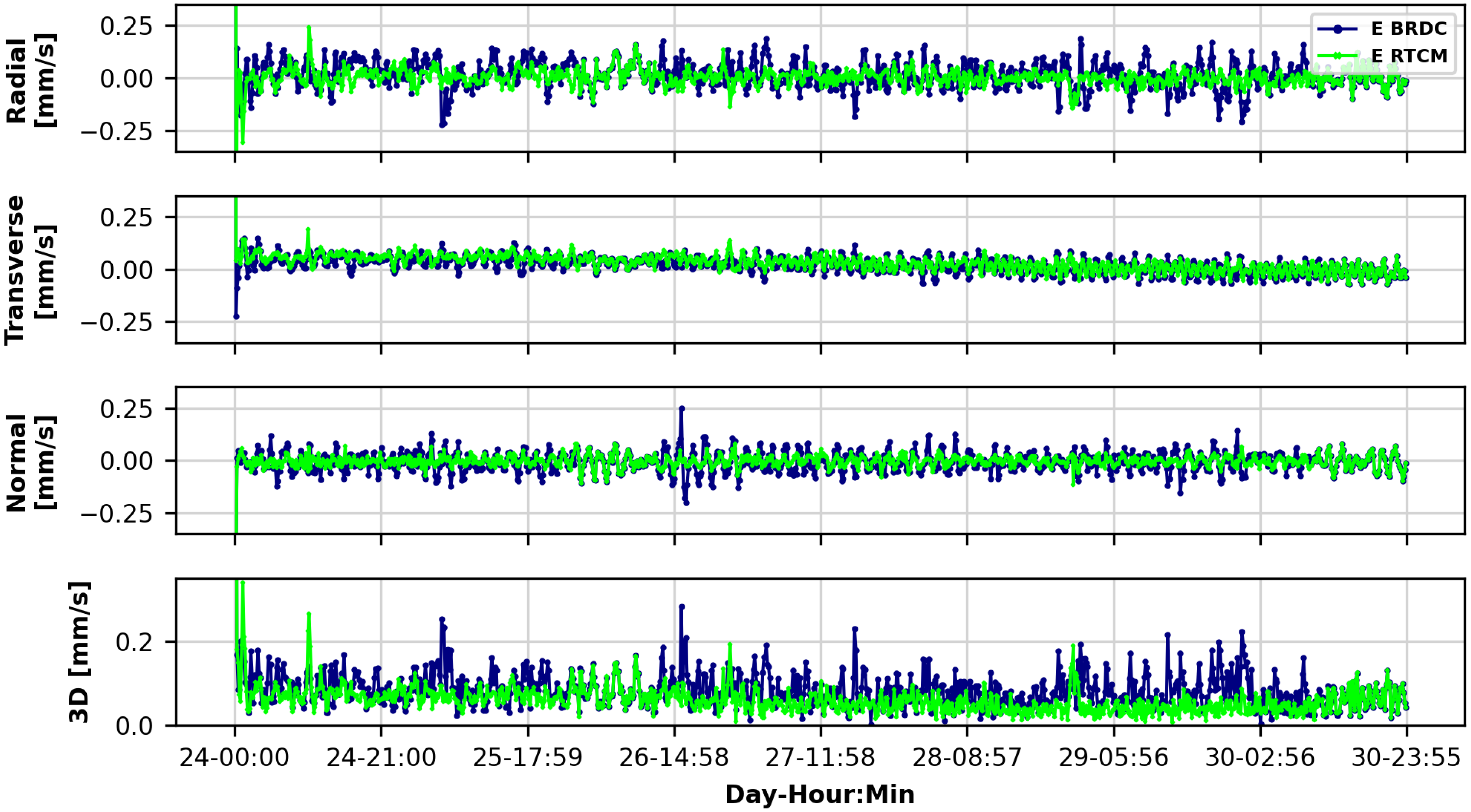
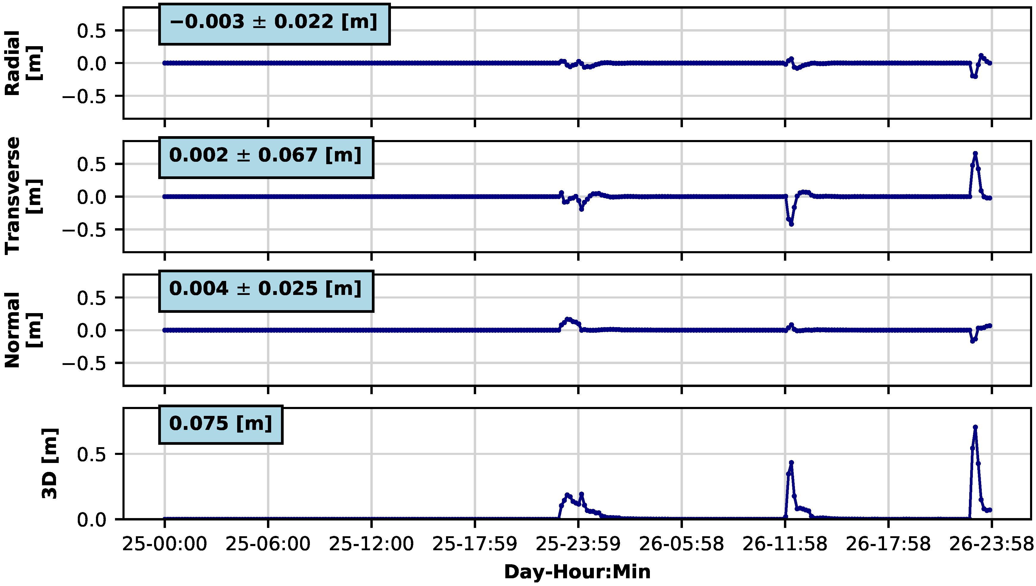
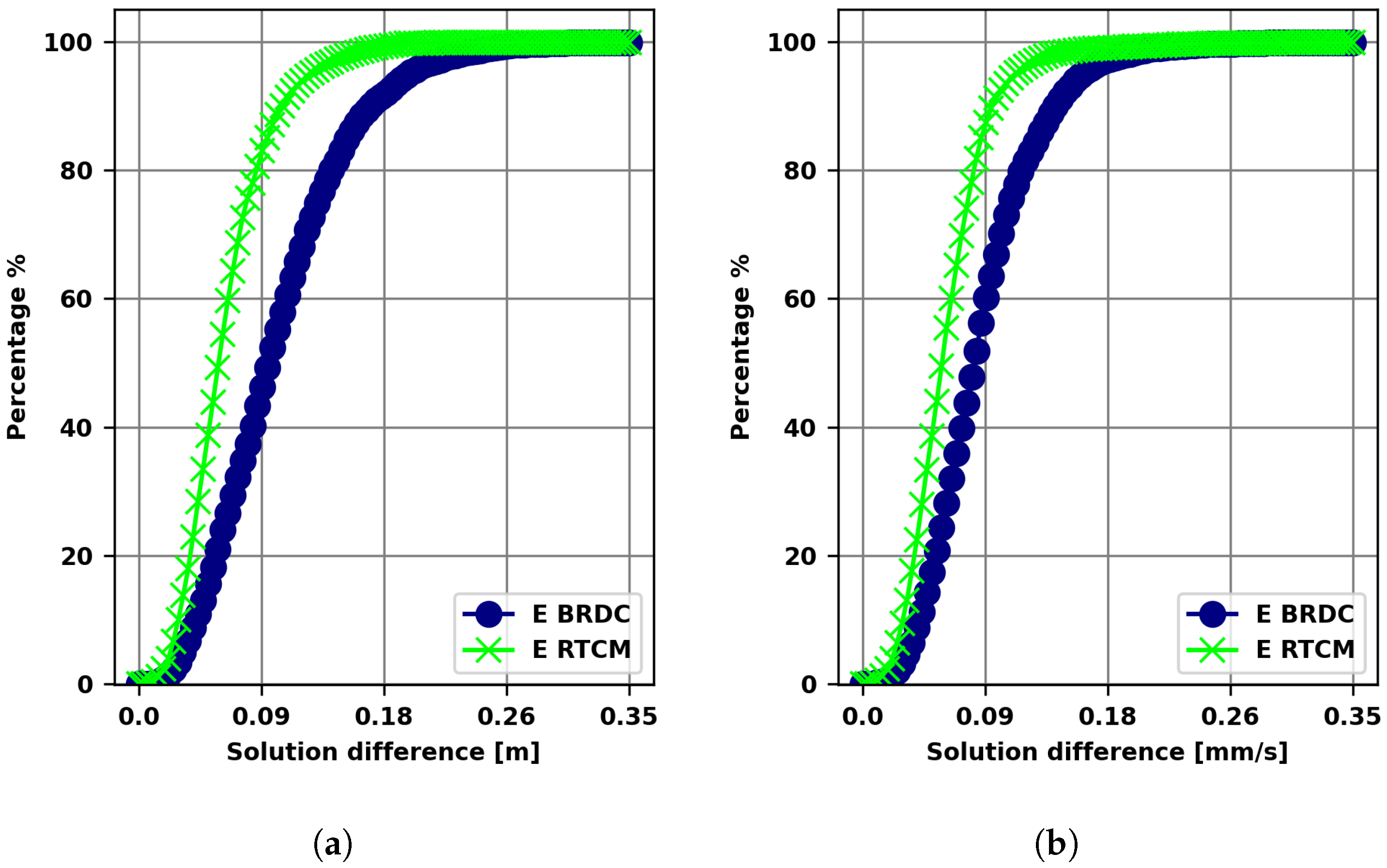
4.2. Spacecraft State Vector Estimation Performance

Figure 1 and Figure 2 show the difference between the UNIPD computation and the CNES-POD solution for 4 September 2021 for position and velocity, respectively. The dynamical state vector obtained in a dual-constellation (GE) configuration without corrections (BRDC, blue-colored curve) is compared to the one resulting from the application of SSR corrections (RTCM, green-colored curve). Figure 1 suggests that the solution benefits from the use of the corrections. Both mean and standard deviation (STD) of the differences decrease in all the directions of the RTN frame. In particular, the STD in transverse and normal directions drops from more than six centimeters to 3.6 cm and 3.1 cm, respectively.

In addition to that, the bottom panel of Figure 1 highlights the improvement in terms of 3D positioning. In fact, the Root Mean Square (RMS) of the 3D difference is reduced by more than four centimeters, passing from 10 cm to 5.7 cm. Similarly, the velocity estimate is improved by adopting the RTCM-SSR corrections. A 3D velocity RMS of 0.078 mm/s is achieved, while a 3D RMS of 0.11 mm/s is obtained when using only the broadcast navigation data. These results embody the potential P2OD solution quality that may be accomplished once this level of quality of SSR corrections is available onboard.

Seven days of S6A Galileo measurements are exploited to assess the P2OD performance in a single-constellation with a Galileo-only configuration. The scenario involves the use of SSR corrections that are not continuously available. This case is actually possible in a real navigation context in which the broadcast correction might be unavailable for some periods.

Figure 3 and Figure 4 exhibit the difference between the UNIPD solution (E BRDC and E RTCM) and the CNES-POD reference solution for position and velocity, respectively.

The results obtained without the aid of SSR (blue-colored curves) are compared to those achieved by applying the corrections (green-colored curves). It can be recognized that during some periods, the two solutions overlap. Specifically, that is the case between 25 September and 26 September and during the second part of the day on 30 September (see Figure 3 and Figure 4). The reason for such behavior is that, in the simulated real-time, no corrections are available during those periods. However, as can be observed, the switch between using and not using the corrections does not cause any discontinuity in the solution. No filter transient is brought about by this discontinuity to adhere to a different accuracy level of GNSS orbits and clocks. Therefore, the results suggest that the strategy with the ambiguity re-initialization adopted in the filter successfully deals with SSR data outages. Figure 5 highlights the effectiveness of the strategy. It shows the difference between applying and not applying the re-initialization method. It can be observed that without re-initialization a filter transient is introduced with peaks in the 3D position solution larger than half a meter.

Looking at Figure 3, the improvement generated by the use of the corrections is generally highlighted in the transverse and normal directions. This behavior is supported by the values reported in

Table 3. Position difference statistics for 24–30 September 2021. For each configuration, the difference is computed with respect to the CNES-POD solution. For the individual axes (RTN frame), the mean values ± standard deviation of the differences are provided. The 95th percentiles are calculated for the position (3D) differences. The filter transient is not included.

Configuration	Radial [mm]	Transverse [mm]	Normal (mm)	3D Position (RMS) (mm)	95th Percentile (mm)
E BRDC	31 ± 37	−19 ± 79	11 ± 55	110	190
E RTCM	19 ± 29	−12 ± 46	3 ± 31	69	119

, with a reduction of the STD from 79 mm to 46 mm and from 55 mm to 31 mm for the transverse and normal directions, respectively. Similar behavior is observed for the radial and normal directions in the velocity domain shown in Figure 4.

As described by

Table 4. Velocity difference statistics for 24–30 September 2021. For each configuration, the difference is computed with respect to the CNES-POD solution. For the individual axes (RTN frame), the mean values ± standard deviation of the differences are provided. The 95th percentile is calculated for the velocity (3D) differences. The filter transient is not included.

Configuration	Radial ($\mathsf{\mu }$m/s)	Transverse ($\mathsf{\mu }$m/s)	Normal ($\mathsf{\mu }$m/s)	3D Position (RMS) ($\mathsf{\mu }$m/s)	95th Percentile ($\mathsf{\mu }$m/s)
E BRDC	15 ± 65	22 ± 38	−5 ± 48	93	155
E RTCM	3 ± 38	29 ± 36	−3 ± 27	66	106

, the STD in radial and normal directions drops from 65 mm to 38 mm and from 48 mm to 27 mm, respectively. Regarding the 3D position and velocity differences, the bottom panels of Figure 3 and Figure 4, respectively, illustrate the variation in time. The use of SSR corrections (for the periods of availability) marks a reduction of the 3D RMS for both position (see Table 3) and velocity (see Table 4). A 3D position RMS of 11 cm is reduced to 6.9 cm when applying the SSR messages. In a similar manner, the 3D velocity RMS decreases from 0.093 mm/s to 0.066 mm/s when correcting the broadcast ephemerides.

Additionally, Table 3 and Table 4 include the 95th percentile of the 3D position and velocity, respectively. While E BRDC ensures a value just below 20 cm, E RTCM allows achieving a 95th percentile slightly below 12 cm. Moreover, the E RTCM solution provides a 95th percentile of the 3D velocity of about 0.1 mm/s.

The distribution of the 3D differences between the UNIPD and the CNES-POD solutions is further analyzed by looking at Figure 6a,b. These figures show the percentage of differences (y-axis) below a certain amount (x-axis). Both Figure 6a,b indicate that the E RTCM curve is steeper than the E BRDC curve. It can be recognized that all the E RTCM differences are below 18 cm and 0.18 mm/s for position and velocity, respectively; 60% of all the E RTCM differences are below 7 cm, while the E BRDC curve reaches the 60% level at roughly 11 cm. Concerning velocity, 60% of the E BRDC solutions are below 0.09 mm/s, and application of the corrections (i.e., E RTCM configuration) diminishes the value to 0.07 mm/s.

Finally, it is worth mentioning that the phase-bias corrections are successfully applied. Although some discontinuities (i.e., phase-bias jumps for a specific satellite) occurred, the ambiguity-strategy reset is demonstrated as effective in avoiding discrepancies in the solution, generating a filter transient similar to the behavior of a data correction outage.

This has no impact on the orbit determination with float ambiguities, but it becomes relevant once the ambiguities need to be fixed to an integer value. Therefore, the approach paves the way to including an IAR algorithm. The IAR analysis will be part of future developments of this investigation.

5. Conclusions

Actual flight data from the Sentinel-6A satellite together with CNES RTCM-SSR corrections data are used to assess the potential of onboard POD based on broadcast ephemerides with SSR augmentation. Onboard orbit determination solutions are generated using the University of Padua SW and compared to the publicly available CNES-SSALTO POD Sentinel-6A reference orbits. By applying the SSR corrections, a 3D position difference RMS of 5.7 cm is obtained in a GPS/Galileo dual-constellation configuration. Concerning velocity, a 3D RMS of 0.078 mm/s is achieved. The results indicate that, once the same quality of corrections is available onboard (e.g., Galileo HAS), GNSS-based navigation performs similar to ground-based computations based on precise GNSS orbits and clocks.

During real-time onboard operations, SSR correction data outages have to be taken into account. The strategy adopted to deal with the discontinuous use of the corrections involves the re-initialization of the carrier-phase ambiguities and an appropriate use of the ambiguity process noise (active only without corrections). This solution avoids the occurrence of a new filter transient that would otherwise appear, and it maintains the orbit determination precision. Such an approach is validated successfully in a Galileo-only, single-constellation configuration. In this scenario, the UNIPD SW meets the needs of onboard POD by reaching RMS values of 6.9 cm and 0.066 mm/s for 3D position and velocity, respectively.

Finally, phase-bias corrections are included in the processing to prepare the algorithm for future IAR development. A technique to handle phase-bias jumps is proposed and validated. This opens the possibility to fix ambiguities in onboard processing, possibly further improving the precision of the current performance. Foreseen future work will involve the assessment of HAS corrections and the adoption of an IAR algorithm. In summary, the UNIPD P2OD SW is shown as a ready-to-fly navigation tool capable of achieving sub-decimeter onboard orbit determination in a Galileo-only configuration.

References

1. Li, B.; Ge, H.; Ge, M.; Nie, L.; Shen, Y.; Schuh, H. LEO enhanced Global Navigation Satellite System (LeGNSS) for real-time precise positioning services. Adv. Space Res. 2019, 63, 73–93. [Google Scholar] [CrossRef]
2. Li, M.; Xu, T.; Guan, M.; Gao, F.; Jiang, N. LEO-constellation-augmented multi-GNSS real-time PPP for rapid re-convergence in harsh environments. GPS Solut. 2022, 26, 29. [Google Scholar] [CrossRef]
3. Scharroo, R.; Bonekamp, H.; Ponsard, C.; Parisot, F.; von Engeln, A.; Tahtadjiev, M.; de Vriendt, K.; Montagner, F. Jason continuity of services: Continuing the Jason altimeter data records as Copernicus Sentinel-6. Ocean Sci. 2016, 12, 471–479. [Google Scholar] [CrossRef] [Green Version]
4. Donlon, C.J.; Cullen, R.; Giulicchi, L.; Vuilleumier, P.; Francis, C.R.; Kuschnerus, M.; Simpson, W.; Bouridah, A.; Caleno, M.; Bertoni, R.; et al. The Copernicus Sentinel-6 mission: Enhanced continuity of satellite sea level measurements from space. Remote Sens. Environ. 2021, 258, 112395. [Google Scholar] [CrossRef]
5. Montenbruck, O.; Kunzi, F.; Hauschild, A. Performance assessment of GNSS-based real-time navigation for the Sentinel-6 spacecraft. GPS Solut. 2022, 26, 12. [Google Scholar] [CrossRef]
6. Darugna, F.; Casotto, S.; Bardella, M.; Sciarratta, M.; Zoccarato, P.; Giordano, P. Sentinel-6A GPS and Galileo Dual-Frequency Real-Time Reduced-Dynamics P2OD. In Proceedings of the 2022 10th Workshop on Satellite Navigation Technology (NAVITEC), Noordwijk, The Netherlands, 5–7 April 2022; pp. 1–12. [Google Scholar] [CrossRef]
7. Hauschild, A.; Montenbruck, O. Precise real-time navigation of LEO satellites using GNSS broadcast ephemerides. Navig. J. Inst. Navig. 2021, 68, 419–432. [Google Scholar] [CrossRef]
8. Montenbruck, O.; Steigenberger, P.; Hauschild, A. Multi-GNSS signal-in-space range error assessment—Methodology and results. Adv. Space Res. 2018, 61, 3020–3038. [Google Scholar] [CrossRef]
9. Carlin, L.; Hauschild, A.; Montenbruck, O. Precise point positioning with GPS and Galileo broadcast ephemerides. GPS Solut. 2021, 25, 77. [Google Scholar] [CrossRef]
10. European Union. Galileo High Accuracy Service Signal-In-Space Interface Control Document (Galileo HAS SIS ICD), 2022. Issue 1.0. Available online: https://www.gsc-europa.eu/sites/default/files/sites/all/files/Galileo_HAS_SIS_ICD_v1.0.pdf (accessed on 15 November 2022).
11. Hauschild, A.; Montenbruck, O.; Steigenberger, P.; Martini, I.; Fernandez-Hernandez, I. Orbit determination of sentinel-6A using the Galileo high accuracy service test signal. GPS Solut. 2022, 26, 120. [Google Scholar] [CrossRef]
12. RTCM Special Committee No. 104; RTCM Standard 10403.3 Differential GNSS (Global Navigation Satellite Systems) Services-Version 3; RTCM: Arlington, VA, USA, 2016.
13. Wang, Z.; Li, Z.; Wang, L.; Wang, N.; Yang, Y.; Li, R.; Zhang, Y.; Liu, A.; Yuan, H.; Hoque, M. Comparison of the real-time precise orbit determination for LEO between kinematic and reduced-dynamic modes. Measurement 2022, 187, 110224. [Google Scholar] [CrossRef]
14. Casotto, S.; Bardella, M.; Zoccarato, P.; Giordano, P. Real Time Reduced-Dynamics POD for LEO Satellites from GNSS Measurements. In Proceedings of the 2018 9th Workshop on Satellite Navigation Technology (NAVITEC), Noordwijk, The Netherlands, 5–7 December 2018. [Google Scholar]
15. GOMspace. GOMX-5 Mission. 2019. Available online: https://gomspace.com/news/payload-collaboration-initiated-for-the-gomx-.aspx (accessed on 15 November 2022).
16. Bastos, C.; Fernandes, R.; Prata, R.; Palomo, J.; Fernandez, A.; Darugna, F.; Bardella, M.; Sciarratta, M.; Casotto, S.; Giordano, P.; et al. Triple-band GNSS Receiver with E6 HAS corrections for Precise Onboard Orbit Determination in LEO. In Proceedings of the 34th International Technical Meeting of the Satellite Division of The Institute of Navigation (ION GNSS+ 2021), St. Louis, MO, USA, 20–24 September 2021; pp. 1053–1065. [Google Scholar]
17. Cullen, R. Sentinel-6A POD Context, 2021. JC-TN-ESA-0420, v1.4; European Space Research and Technology Centre, European Space Agency: Noordwijk, The Netherlands, 2021. [Google Scholar]
18. IGS/RTCM. RINEX—The Receiver Independent Exchange Format Version 3.04. International GNSS Service (IGS), RINEX Working Group and Radio Technical Commission for Maritime Services Special Committee 104 (RTCM–SC104). 2018. Available online: https://files.igs.org/pub/data/format/rinex304.pdf (accessed on 15 November 2022).
19. Steigenberger, P.; Montenbruck, O.; Hessels, U. Performance evaluation of the early CNAV navigation message. Navig. J. Inst. Navig. 2015, 62, 219–228. [Google Scholar] [CrossRef]
20. Yunck, T.P.; Melbourne, W.G.; Thornton, C. GPS-based satellite tracking system for precise positioning. IEEE Trans. Geosci. Remote Sens. 1985, GE-23, 450–457. [Google Scholar] [CrossRef]
21. Wu, S.C.; Yunck, T.P.; Thornton, C.L. Reduced-dynamic technique for precise orbit determination of low earth satellites. J. Guid. Control Dyn. 1991, 14, 24–30. [Google Scholar] [CrossRef]
22. Yunck, T.; Bertiger, W.; Wu, S.; Bar-Sever, Y.; Christensen, E.; Haines, B.; Lichten, S.; Muellerschoen, R.; Vigue, Y.; Willis, P. First assessment of GPS-based reduced dynamic orbit determination on TOPEX/Poseidon. Geophys. Res. Lett. 1994, 21, 541–544. [Google Scholar] [CrossRef]
23. van den IJssel, J.; Encarnação, J.; Doornbos, E.; Visser, P. Precise science orbits for the Swarm satellite constellation. Adv. Space Res. 2015, 56, 1042–1055. [Google Scholar] [CrossRef]
24. Förste, C.; Bruinsma, S.; Flechtner, F.; Abrykosov, O.; Dahle, C.; Marty, J.; Lemoine, J.; Biancale, R.; Barthelmes, F.; Neumayer, K.; et al. EIGEN-6C3-The latest Combined Global Gravity Field Model including GOCE data up to degree and order 1949 of GFZ Potsdam and GRGS Toulouse. In AGU Fall Meeting Abstracts; EGU General Assembly: Vienna, Austria, 2011; Volume 2011, p. G51A-0860. Available online: https://ui.adsabs.harvard.edu/abs/2014EGUGA..16.3707F/abstract (accessed on 15 November 2022).
25. McCarthy, D.; Petit, G. IERS Technical Note No.32; Verlag des BKG: Frankfurt, Germany, 2003. [Google Scholar]
26. Tapley, B.; Shutz, B.; Born, G. Statistical Orbit Determination; Elsevier Academic Press: San Diego, CA USA, 2004. [Google Scholar]
27. Hull, D.G. Fourth-order Runge-Kutta integration with stepsize control. AIAA J. 1977, 15, 1505–1507. [Google Scholar] [CrossRef]
28. Wu, J.; Wu, S.; Hajj, G.; Bertiger, W.; Lichten, S. Effects of antenna orientation on GPS carrier phase. Manuscr. Geod. 1993, 18, 91–98. [Google Scholar]
29. Montenbruck, O.; Markgraf, M.; Naudet, J.; Santandrea, S.; Gantois, K.; Vuilleumier, P. Autonomous and precise navigation of the PROBA-2 spacecraft. In Proceedings of the AIAA/AAS Astrodynamics Specialist Conference and Exhibit, Honolulu, HI, USA, 18–21 August 2008; p. 7086. [Google Scholar]
30. Wang, F.; Gong, X.; Sang, J.; Zhang, X. A novel method for precise onboard real-time orbit determination with a standalone GPS receiver. Sensors 2015, 15, 30403–30418. [Google Scholar] [CrossRef] [PubMed]
31. CNES-SSALTO/POD. Sentinel-6A CNES POD Orbital Solution. 2021. Available online: https://cddis.nasa.gov/archive/doris/products/orbits/ssa/s6a/ (accessed on 12 February 2022).
32. EUMETSAT. Sentinel-6 A GNSS-RO NTC Cal/Val Report. EUM/LEO-JASCS/REP/21/1243117, v1C. 2021. Available online: https://www-cdn.eumetsat.int/files/2021-11/Sentinel-6%20A%20GNSS-RO%20NTC%20Cal_Val%20Report.pdf (accessed on 14 November 2022).
Figure 1. S6A orbital position difference with respect to CNES-POD reference solution on 4 September 2021. Two solutions are compared: the first is obtained by using only broadcast navigation data (blue-colored lines), and the second is found by correcting the broadcast navigation data using RTCM corrections from CNES (green-colored lines). For the individual axes (RTN frame), the mean values ± standard deviation of the differences are provided (light-blue-filled boxes for BRDC and light-green-filled boxes for RTCM). The RMS value is shown for the 3D panel.
Remotesensing 14 06121 g001
Figure 2. S6A orbital velocity difference with respect to CNES-POD reference solution on 4 September 2021. Two solutions are compared: the first is obtained by using only broadcast navigation data (blue-colored lines), and the second is found by correcting the broadcast navigation data using RTCM corrections from CNES (green-colored lines). For the individual axes (RTN frame), the mean values ± standard deviation of the differences are provided (light-blue-filled boxes for BRDC and light-green-filled boxes for RTCM). The RMS value is shown for the 3D panel.
Remotesensing 14 06121 g002
Figure 3. S6A orbital position difference with respect to CNES-POD reference solution from 24 September to 30 September 2021. Two solutions are compared: one is obtained using only broadcast navigation data (blue-colored lines), and the other is found by correcting the broadcast navigation data using RTCM corrections from CNES (green-colored lines).
Remotesensing 14 06121 g003
Figure 4. S6A velocity difference with respect to CNES-POD reference solution from 24 September to 30 September 2021. Two solutions are compared: one is obtained using only broadcast navigation data (blue-colored lines), and the other is found by correcting the broadcast navigation data using RTCM corrections from CNES (green-colored lines).
Remotesensing 14 06121 g004
Figure 5. Solution difference between applying and not applying the ambiguity re-initialization. For the individual axes (RTN frame), the mean values ± standard deviation of the differences are provided. The RMS value is shown for the 3D panel.
Remotesensing 14 06121 g005
Figure 6. (a) Cumulative 3D position differences between UNIPD and CNES-POD solutions. (b) Cumulative 3D velocity differences between UNIPD and CNES-POD solutions.
Remotesensing 14 06121 g006