Using a Remote-Sensing-Based Piecewise Retrieval Algorithm to Map Chlorophyll-a Concentration in a Highland River System

Abstract

Chlorophyll-a(chl-a) has been used as an important indicator of water quality. Great efforts have been invested to develop remote-sensing-based chl-a retrieval models. However, due to the spatial difference in chl-a concentration, a single model usually cannot accurately predict the whole range of chl-a concentration. To test the performance of precedent chl-a models, we carried out an experiment along the upper and middle reaches of the Kaidu River and around some small ponds in the Bayanbulak Wetland. We measured water surface reflectance in the field and analyzed the chl-a concentration in the laboratory. Initially, we performed a sensitivity analysis of the spectrum band to chl-a concentration with the aim of identifying the most suitable bands for various chl-a models. We found that the water samples could be divided into two groups with a threshold of 4.50 mg/m³. Then, we tested the performance of 11 precedent chl-a retrieval models and 7 spectral index-based regression models from this study for all the sample datasets and the two separate datasets with relatively high and low chl-a concentrations. Through a complete comparison of the performance of these models, we selected the D3B model for water bodies with high chl-a concentration and OC2 model (ocean color 2) for low chl-a concentration waters, resulting in the hierarchical and piecewise retrieval algorithm OC2-D3B. The chl-a concentration of 4.50 mg/m³ corresponded to the D3B value of −0.051; therefore, we used −0.051 as the threshold value of the OC2-D3B model. The result of the OC2-D3B model showed a better performance than the other algorithms. Finally, we mapped the spatial distribution and seasonal pattern of chl-a concentration in Bayanbulak Wetland using Sentinel-2 images from 2016 to 2019. The results indicated that the chl-a concentration in the riparian ponds was generally in the range of 8–10 mg/m³, which was higher than that in rivers with a range of 2–4 mg/m³. The highest chl-a concentration usually appears in summer, followed by spring and autumn, and the lowest in winter. The correlation between meteorological data and chl-a concentration showed that temperature is the dominant factor for chl-a concentration changes. Our analytical framework could provide a better way to accurately map the spatial distribution of chl-a concentration in complex river systems.

1. Introduction

The concentration of chlorophyll a (chl-a) has been extensively used to reflect water transparency, the degree of eutrophication and the biomass of phytoplankton [1,2,3,4,5,6,7]. The rapid and accurate determination of chl-a concentration in a wide range of water bodies is important in water environment monitoring. Compared with the traditional water quality monitoring method based on field investigation, remote sensing technology has the advantages of a low cost, wide range and high efficiency. With the development of high-resolution and multi-source satellite sensors, the retrieval of water-environment-related elements using remote sensing has been widely applied in the monitoring of water quality and hydro-environmental pollution in large areas of water [8,9,10,11,12,13,14,15,16,17].

Previous studies have proposed a variety of chl-a-retrieving algorithms for different optical types of waters. Generally, these algorithms can be grouped into three categories: empirical models, semi-analytical models and analytical models [18,19]. The ocean color algorithm OCx [2,7], SVM model [20] and LSTM model [21] are among the most commonly used empirical models. The semi-analytical models include a two-band model [22], three-band model [23,24,25], four-band model [26] and APPLE model [27]. In addition to these models, the Fluorescence Line Height (FLH) [28], Maximum Chlorophyll Index (MCI) [29] and Comprehensive Chlorophyll Index (SCI) [30] based on chlorophyll fluorescence characteristics were also used to capture the chl-a concentration. The basic principle of these algorithms is to build strong linkage between the reflectance of sensitive bands and the chl-a concentration in water [5]. However, the spatial heterogeneity of the optical properties and chl-a concentration of the waters makes these algorithms hard to apply universally. To overcome the disadvantages of the traditional models, machine learning has been used to enhance the predictability of remote-sensing-based chl-a models [31,32,33,34,35,36]. Due to the limitations of data availability over a large area, the machine-learning-based algorithms usually work regionally.

In recent decades, investigations of remote sensing estimations of chl-a concentration in waters have mainly been concentrated in large-scale open areas such as oceans, coastal seas or relatively static inland lakes [6,26,37,38,39,40]. In contrast, there were relatively few focusing on rivers with varying flow rates and rapidly changing water quality. The river channel is relatively narrow and could only cover a few pixels for low–medium-resolution satellite images, which will bring great uncertainty to the results. Despite the development of aerial photogrammetry, the high cost prevents us from implementing the field survey over a large-scale area. Moreover, the high variability of the water composition resulting from climate change and human disturbance makes it difficult to capture the conditions of water quality. However, an experiment should be conducted in a complex river system to validate the traditional model or algorithm.

In Class I water bodies, such as oceans, which are mainly composed of phytoplankton and its secondary products, the optical characteristics (namely, absorption and scattering) of chl-a in the blue and green bands are distinctly displayed on the spectrum curve. However, in Class II water bodies with complex optical properties, the optical characteristics of chl-a in the same bands are masked by the strong absorption of high-concentrated Colored Dissolved Organic Matter (CDOM) and Non-Algal Particles (NAP) in the water. Additionally, in the red near-infrared band, the absorption of CDOM and NAP sharply decreases, and the absorption proportion of chl-a greatly increases, finally forming the obvious spectral peak–valley feature [41]. Therefore, the chl-a algorithm based on specific bands cannot balance the optical characteristics of multiple types of water bodies. Some studies have tried to classify the waters into different types in order to achieve the best modelling results. For example, based on the degree of eutrophication, biomass and turbidity, we can divide the waters in the same region into different types to establish an integrated model, which could be generally applied to each water type [6,39,42,43,44]. This kind of model could compensate for the shortcomings of using a single algorithm for different types of water.

The Bayanbulak river basin has complex river systems, with the coexistence of both river- and pond-like wetlands. The topography in the river basin is relatively flat and the terrains along the river channel tend to be flooded. Many ponds are distributed along the adjacent riparian belt. It is of scientific significance to map the chl-a concentration in this complex river system. In this study, we aimed to establish an integrated model to simulate the chl-a concentration in a river–wetland interlinked fluvial system through a comprehensive analysis of field-measured water surface reflectance spectrum and chl-a concentration. Then, we utilized long time-series Sentinel-2 images to capture the spatial and temporal variations in chl-a concentrations in Bayanbulak basin. Finally, we determined the major driver of chl-a concentration variation.

2. Materials and Methods

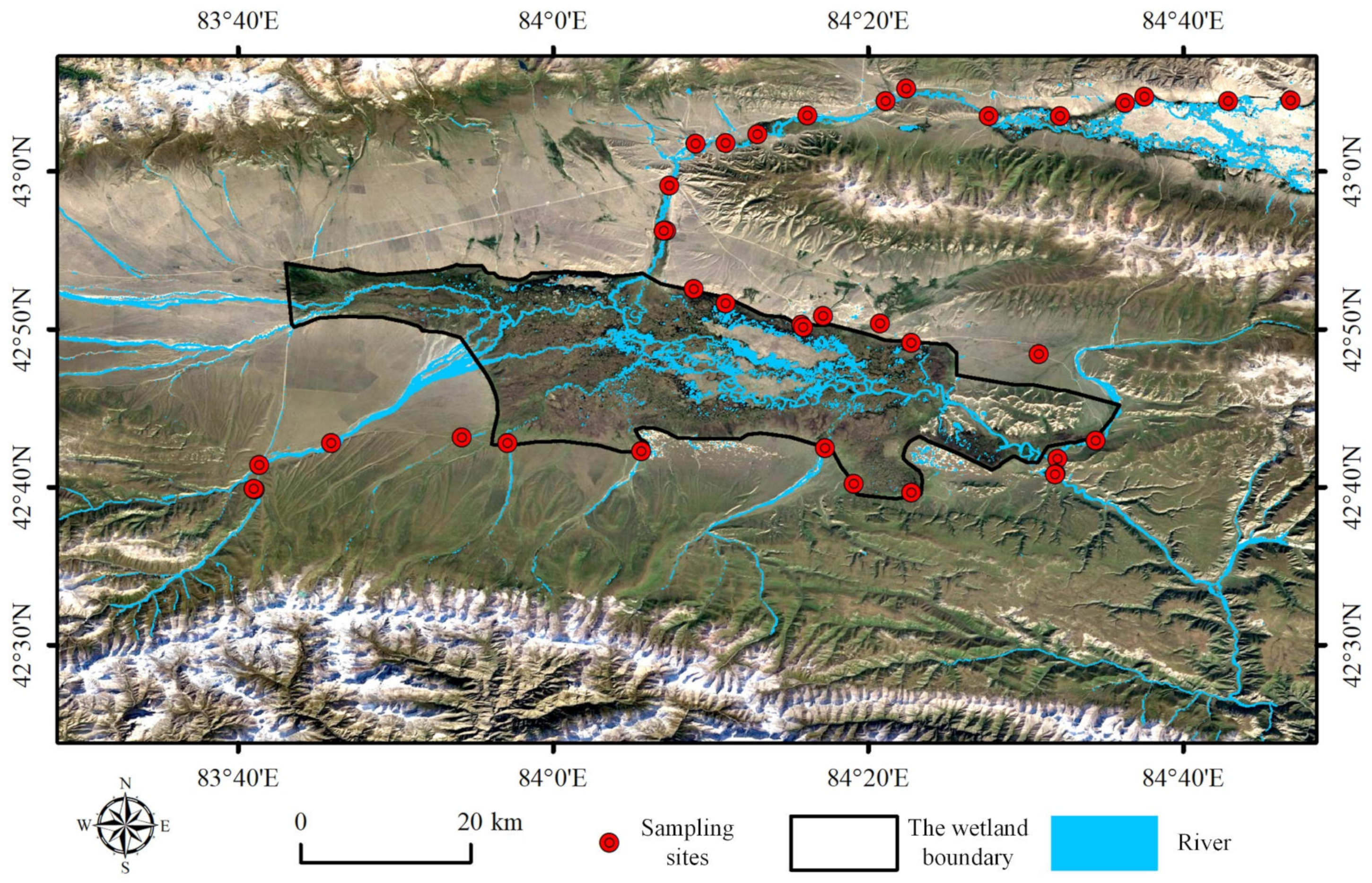
2.1. Study Area

The study area, Bayanbulak marshy meadow, is in the northwest of Hejing County in Xinjiang (Figure 1), which is in the central mountain basin of the Tianshan Mountains, with an average altitude of about 2500 m and a total area of about 15,000 km². The mean annual temperature was −4.5 °C, and the average temperature from April to September was 5–10 °C. The land is mainly covered by typical alpine meadow grassland and is the largest alpine grassland in China. Natural precipitation and the melt waters of glacier and snow in Tianshan are the main supplies of water resources in wetlands. Due to the influence of natural resources exploitation and rising temperature in these areas, the overall wetland area was degraded from 1996 to 2015 [45]. Field investigation observed that grassland degradation and desertification occurred in some places within the wetland.

2.2. Data

2.2.1. Field Spectral Data Measurement and Water Sample Collection

During the field work, we collected 38 water samples from the main river channel and the small riparian ponds in the middle and upper reaches of the Kaidu River from 16 July to 29 July 2018. For each sample, a volume of 1000 mL was collected and stored in a dark environment at 0~4 °C. Then, we took these samples to the laboratory to extract chl-a concentration. The summarized information of chl-a concentration is shown in

Table 1. Descriptive statistics of the chl-a concentration of the samples.

Samples	Min (mg/m3)	Max (mg/m3)	Mean (mg/m3)	STD (mg/m3)	CV	Number of Samples
Total	2.53	8.72	4.29	1.65	0.39	38
Main River	2.78	8.06	4.16	1.37	0.33	12
Ponds	2.53	8.72	5.33	1.98	0.37	13
Tributaries	2.67	5.24	3.37	0.67	0.20	13

STD: Standard Deviation. CV: Coefficient of Variance.

.

The chl-a concentration for all samples was less than 10.00 mg/m³ (Table 1). In all 38 samples, the chl-a concentration of 26 samples was 2.00~4.50 mg/m³, showing that the overall chl-a concentration in wetland water was low. Generally, water bodies with a chl-a concentration of 2.60~7.20 mg/m³ were considered to have medium eutrophication, and those within the range 1.00~2.60 mg/m³ had poor eutrophication [46]. According to this standard, the water body in this study can be regarded as having low–medium eutrophication.

In the field, we simultaneously measured the water spectra using the Analytical Spectral Devices (ASDs) FieldSpec^® 3 field portable spectrometer (Malvern Panalytical, Malvern, UK) when we collected water samples for laboratory analysis. This spectrometer has a surveying wavelength ranging from 350 to 2500 nm. The sampling interval was 1.4 nm in the range of 350–1000 nm, and 2 nm in the range of 1001–2500 nm [47]. The ASD spectroradiometer was initially calibrated at each sampling site before taking the measurement. Then, we measured the spectrums from the reference whiteboard and river water surface at each site. The measurement was taken at a 30 cm height above the surface in a vertical downward direction under clear-sky conditions [47]. The reference whiteboard was placed on a flat surface. Ten spectral measurements were taken consecutively to minimize random errors from the surrounding environment. Water bodies are weak radiators with a lower reflectance than other land-cover types. The mixed spectrums from turbid water, river bottom, and adjacent land surfaces were complicated due to variations in stream width, depth, and velocity [47]. To reduce the interference from the river bottom and surrounding objects, we chose relatively deep water.

The measurement method in the field was the above-water observation method [48], which can effectively reduce the influences of direct solar radiation and the surrounding environment. The optical physical parameters in the field measurements consisted of above-water total upward radiance $L\left(\lambda \right)$, total incident irradiance $E_d\left(0^{+}\right)$, and downward scattered radiance $L_p\left(\lambda \right)$ of sky light. $E_d\left(0^{+}\right)$ is obtained by measuring the radiance brightness $L_G\left(\lambda \right)$ of the standard reference plate, and the remote sensing reflectance of the water body ($R_{rs}\left(\lambda \right)$) is calculated based on the measured physical variables using Equation (1)

$$R_{rs}\left(\lambda \right)=\frac{L_w\left(\lambda \right)}{E_d\left(0^{+}\right)}=\frac{L\left(\lambda \right)-\rho \times L_p\left(\lambda \right)}{L_G\left(\lambda \right)\times \pi /{\rho }_b}\times 100\%$$

(1)

where $\lambda$ is the wavelength. $L_w\left(\lambda \right)$ represents the water-leaving radiance, which is acquired from $L\left(\lambda \right)$. $\rho$ is the reflectance of the air–water interface, which is related to the solar zenith angle, wind speed, observation angle and water surface roughness, etc. ${\rho }_b$ is the corrected reflectance of the reference plate.

There were a total of 38 sampling sites in the field for water surface reflectance spectral data. Of all the samples, two samples were eliminated because they had apparently incorrect spectral curves due to interference from the measurement environment. Figure 2a,b represents the remote sensing reflectance spectrum of sampling sites with chl-a ≤ 4.50 mg/m³ and >4.50 mg/m³. Generally, the ranges of spectrum curves for different band significantly varied. However, the “peak–valley” shape of the spectrum was like that reported in the literature [5,9,39,49,50]. The reflectance of the visible band is higher than that of the near-infrared band. The strong absorption of the components in the water results from the low reflectance of the blue band. The reflectance was enhanced as the wavelength increased. The reflectance spectrum peaked at about 455 nm. The reflectance reached its highest peak at around 550~580 nm, which arose due to the scattering caused by phytoplankton and suspended particles. From the red band to the near-infrared band, the overall spectral reflectance decreases because of the absorption of hydrogen.

Notably, chl-a shows strong absorption at around 675 nm, while NAP and CDOM have weaker absorption. Therefore, the reflectance spectrum of water with high chl-a concentration (Figure 2b) will form a chl-a spectrum valley. The peak at around 700 nm results from the fluorescence due to the photosynthesis of phytoplankton after absorbing solar energy. It is an important spectral feature to determine whether the water body contains chlorophyll. From Figure 2a,b, we can observe that, in a water body with chl-a > 4.50 mg/m³, there is a chl-a absorption valley of around 675 nm and fluorescence peak of around 700 nm. In contrast, in the water body with chl-a ≤ 4.50 mg/m³, these features do not appear because the reflectance in the near-infrared band is strongly influenced by other components, which probably conceals the chl-a signal.

2.2.2. Remote-Sensing Data

The remote sensing datasets used in this study are the Sentinel-2 images with a high spatial and temporal resolution provided by the Sentinel Data Center of European Space Agency (ESA) (https://scihub.copernicus.eu/ (accessed on 18 May 2020)). Sentinel-2 consists of two polar orbit satellites, 2A and 2B, and is equipped with a Multi-Spectral Instrument (MSI) with 13 wavelength bands, from visible and near-infrared to short-wave infrared. MSI has three spatial resolutions (10 m, 20 m, 50 m) for different bands. The width of each image scene is 290 km. The revisiting period of the same satellite is 10 days, and when two satellites observe the same area, the revisiting period is reduced to 5d. The downloaded Sentinel-2 L1C level images were geometrically corrected and radiometrically calibrated. In order to obtain an accurate reflectance of water bodies, the atmospheric effects were corrected using Sen2Cor (version 2.8), a special plug-in for atmospheric correction released by ESA, which is highly consistent with the 6S model [51].

2.2.3. Meteorological Data

This study used daily meteorological data from Bayanbulak meteorological station (84°08′56″E, 40°01′58″N), including temperature, precipitation, and sunshine duration. These datasets were provided by China’s National Meteorological Science Data Center (http://data.cma.cn/ (accessed on 15 June 2020)). For comparison with monthly average chl-a concentrations derived from remote sensing data, we processed the meteorological data into monthly values.

2.3. Methods

2.3.1. The Validation of the Classical Models

We divided water bodies into two categories according to the concentration of chl-a of 4.50 mg/m³, as shown in Figure 2. In this study, we collected 11 types of commonly used chl-a models, an empirical and semi-analytical model, to test their applicability in our study area (

Table 2. Brief descriptions of the 11 types of chl-a retrieval algorithms used in this study.

Model	Equation
Tchl-a [7]	$R=R_{rs}\left(433\right)/R_{rs}\left(555\right)\ast {\left(R_{rs}\left(412\right)/R_{rs}\left(490\right)\right)}^{C_0}$ $Chl–a={10}^{\left(c_1+c_{2}Lo{g}_{10}\left(R\right)+C_{3}Lo{g}_{10}^2\left(R\right)\right)}$ $C_0=-0.935, C_1=0.342, C_2=-2.511, C_3=-0.277$
OC2V4 [2]	$R=Lo{g}_{10}\left(max\left(R_{rs}\left(443\right),R_{rs}\left(490\right)\right)/R_{rs}\left(560\right)\right)$ $Chl–a={10}^{\left(c_0+c_{1}R+c_2{R}^2+c_3{R}^3+c_4{R}^4\right)}$ $C_0=0.2975, C_1=-21.502, C_2=-215.53, C_3=-784.5, C_4=-859.7$
OC4V4 [2]	$R=Lo{g}_{10}\left(max\left(R_{rs}\left(443\right),R_{rs}\left(490\right),R_{rs}\left(510\right)\right)/R_{rs}\left(560\right)\right)$ $Chl–a={10}^{\left(c_0+c_{1}R+c_2{R}^2+c_3{R}^3+c_4{R}^4\right)}$ $C_0=-0.599, C_1=-50.54, C_2=-578.38, C_3=-2525.7, C_4=-376.2$
NDCI [52]	$NDCI=\left(R_{rs}\left(708\right)-R_{rs}\left(665\right)\right)/\left(R_{rs}\left(708\right)+R_{rs}\left(665\right)\right)$ $Chl–a=4.0448+10.301\ast \left(NDCI\right)$
FLH [28]	$FLH=R_{rs}\left({\lambda }_2\right)-[R_{rs}\left({\lambda }_3\right)+\frac{{\lambda }_2-{\lambda }_3}{{\lambda }_1-{\lambda }_3}\ast \left(R_{rs}\left({\lambda }_1\right)-R_{rs}\left({\lambda }_3\right)\right)]$ ${\lambda }_1:665nm, {\lambda }_2:681nm, {\lambda }_3:708nm$ $Chl–a=3.6268-11.289\ast \left(FLH\right)-17.743\ast {\left(FLH\right)}^2$
MCI [29]	$MCI=L_w\left({\lambda }_2\right)-[L_w\left({\lambda }_1\right)+\frac{{\lambda }_2-{\lambda }_1}{{\lambda }_3-{\lambda }_1}\ast \left(L_w\left({\lambda }_3\right)-L_w\left({\lambda }_1\right)\right)]$ ${\lambda }_1:681nm, {\lambda }_2:708nm, {\lambda }_3:753nm$ $Chl–a=5.6122-2.1844\ast \left(MCI\right)+0.6641\ast {\left(MCI\right)}^2$
SCI [30]	$H_{Chl}=\left[R_{rs}\left({\lambda }_4\right)+\frac{{\lambda }_4-{\lambda }_3}{{\lambda }_4-{\lambda }_2}\left(R_{rs}\left({\lambda }_2\right)-R_{rs}\left({\lambda }_4\right)\right)\right]-R_{rs}\left({\lambda }_3\right)$ $H_{△}=R_{rs}\left({\lambda }_2\right)-\left[R_{rs}\left({\lambda }_4\right)+\frac{{\lambda }_4-{\lambda }_2}{{\lambda }_4-{\lambda }_1}\left(R_{rs}\left({\lambda }_1\right)-R_{rs}\left({\lambda }_4\right)\right)\right]$ $SCI=H_{Chl}-H_{△}\hspace{0.33em}$${\lambda }_1:560nm, {\lambda }_2:620nm, {\lambda }_3:665nm, {\lambda }_4:681nm$ $Chl–a=5.7457-7.9685\ast \left(SCI\right)+5.7043\ast \left(SCI\right)^2$
G2B [22]	$G2B=\frac{R_{rs}\left({\lambda }_2\right)}{R_{rs}\left({\lambda }_1\right)}\hspace{0.33em}$${\lambda }_1:659nm, {\lambda }_2:692nm$ $Chl–a=49.739-124.14\ast \left(G2B\right)+82.754\ast {\left(G2B\right)}^2$
D3B [25]	$D3B=[R_{rs}{\left({\lambda }_1\right)}^{-1}-R_{rs}{\left({\lambda }_2\right)}^{-1}]\ast R_{rs}\left({\lambda }_3\right)$ ${\lambda }_1:659nm, {\lambda }_2:692nm, {\lambda }_3:748nm$ $Chl–a=6.9756+73.431\ast \left(D3B\right)+344.53\ast {\left(D3B\right)}^2$
L4B [26]	$L4B=[R_{rs}{\left({\lambda }_1\right)}^{-1}-R_{rs}{\left({\lambda }_2\right)}^{-1}]/[R_{rs}{\left({\lambda }_4\right)}^{-1}-R_{rs}{\left({\lambda }_3\right)}^{-1}]$ ${\lambda }_1:659nm, {\lambda }_2:692nm, {\lambda }_3:705nm, {\lambda }_4:748nm$ $Chl–a=5.5923+11.566\ast \left(L4B\right)+15.472\ast {\left(L4B\right)}^2$
Gchl-a [44]	$b_b=1.61\ast R_{rs}\left(779\right)/\left(0.082-0.6\ast R_{rs}\left(779\right)\right)$ $Chl–a=\left(R_{rs}\left(709\right)/R_{rs}\left(665\right)\ast \left(0.7+b_b\right)-0.4-b_b^{1.06}\right)/0.016$

). We performed a comparison of these models in order to choose the most suitable model or algorithm.

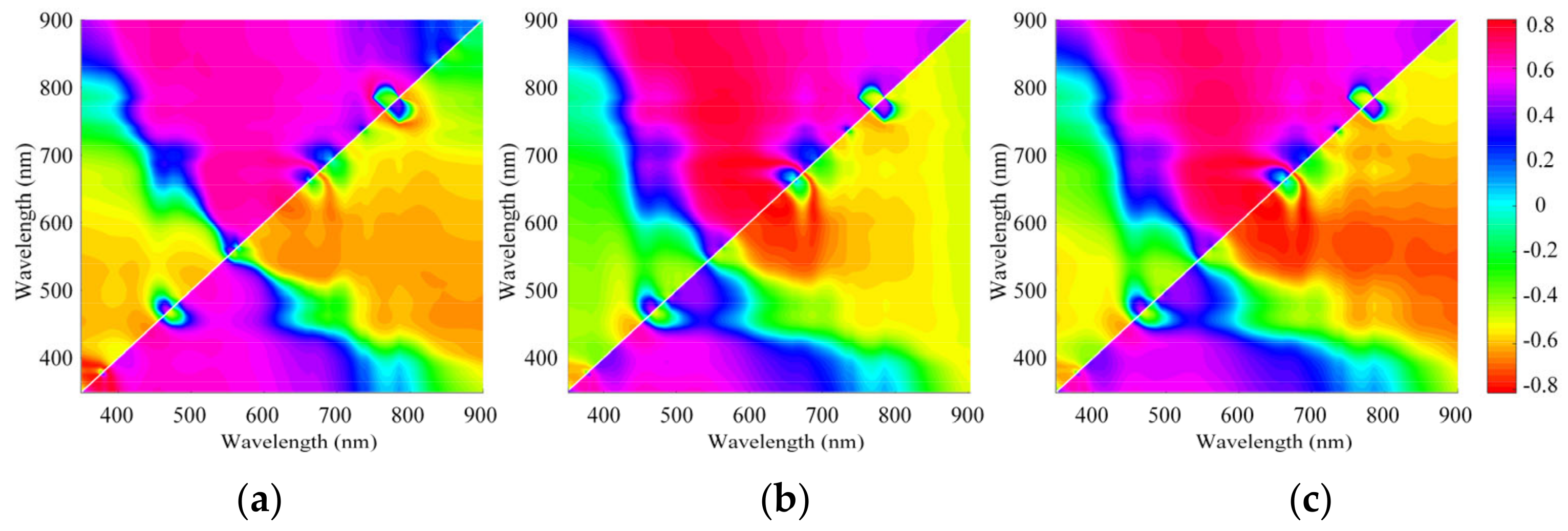
2.3.2. Spectral Index Based Regression Model

The initially calculated $R_{rs}$ could contain noise caused by the environment, measurement angle and other factors. To eliminate the noise, we corrected the originally calculated reflectance by normalization and first-order differential. The average reflectance of from 400 to 900 nm with a stable signal was used as the standard mean value. The ratio of reflectance of each band to the average value was the normalized reflectance $R_n\left(\lambda \right)$. The principle of first-order differential was to obtain the first derivative of the initially calculated $R_{rs}$. We implemented this in the software Origin 2021. Compared with the other processing methods, normalization can effectively enhance the correlation between reflectance and chl-a concentration (Figure 3). In the range of visible bands, the absolute value of the correlation coefficient between normalized reflectance and chl-a concentration between 524 and 576 nm was greater than 0.70, with a maximum of 0.72 at 537 nm and almost zero at 428 nm and 678 nm. We used four forms of spectral indexes, $R_n\left(\lambda \right), R_n\left({\lambda }_1\right)-R_n\left({\lambda }_2\right)$, $R_n\left({\lambda }_1\right)/R_n\left({\lambda }_2\right)$, and $\left(R_n\left({\lambda }_1\right)-R_n\left({\lambda }_2\right)\right)/\left(R_n\left({\lambda }_3\right)+R_n\left({\lambda }_4\right)\right),$ to conceive four models X_I-X₄ with the input of the four specific wavelengths (

Table 3. The optimal fitting equation between reflectance and chl-a concentration based on regression analysis.

Model	Variable	Equation	R2
X1	$X_1=R_n\left(537\right)$	$\mathrm{chl}-\mathrm{a}=3.2765X_1{}^2-0.3799X_1+3.1175$	0.56
X2	$X_2=(R_n\left(537\right)-R_n\left(428\right))$ $/(R_n\left(537\right)+R_n\left(428\right))$	$\mathrm{chl}-\mathrm{a}=14.681X_2{}^2+17.266X_2+8.1809$	0.48
X3	$X_3=\frac{R_n\left(537\right)}{R_n\left(678\right)}$	$\hspace{1em}\mathrm{chl}-\mathrm{a}=8.5277X_3{}^2-0.2788X_3+3.3603$	0.36
X4	$X_4=(R_n\left(537\right)-R_n\left(678\right))$ $/(R_n\left(537\right)+R_n\left(678\right))$	$\hspace{1em}\mathrm{chl}-\mathrm{a}=8.6092X_4{}^2+14.272X_4+9.3707$	0.34
X5	$X_5=(R_{rs}\left(384\right)-R_{rs}\left(385\right))\ast 100$	$\mathrm{chl}-\mathrm{a}=75435X_5{}^2+1063.9X_5+6.896$	0.63
X6	$X_6=R_{rs}\left(689\right)/R_{rs}\left(613\right)$	$\hspace{1em}\mathrm{chl}-\mathrm{a}=107.82X_6{}^2-166.85X_6+67.757$	0.82
X7	$X_7=(R_{rs}\left(625\right)-R_{rs}\left(624\right))$ $/(R_{rs}\left(625\right)+R_{rs}\left(624\right))\ast 100$	$\hspace{1em}\mathrm{chl}-\mathrm{a}=105.97X_7{}^2+45.711X_7+8.2691$	0.73

).

To compare the performance of the normalized reflectance $R_n\left(\lambda \right)$ and the initially calculated $R_{rs}$ in model building, we constructed the $R_{rs}$ based spectral indexes, $R_{rs}\left({\lambda }_1\right)-R_{rs}\left({\lambda }_2\right)$, $R_{rs}\left({\lambda }_1\right)/R_{rs}\left({\lambda }_2\right)$, and $\left(R_{rs}\left({\lambda }_1\right)-R_{rs}\left({\lambda }_2\right)\right)/\left(R_{rs}\left({\lambda }_3\right)+R_{rs}\left({\lambda }_4\right)\right)$ as basic variables to conceive new models. The determination of the specific wavelengths used in these indexes was based on the maximum correlation coefficients between chl-a concentration and the specific spectral indexes (Figure 4). Eventually, we used the three representative spectral indexes, $R_{rs}\left(384\right)-R_{rs}\left(385\right)$, $R_{rs}\left(689\right)/R_{rs}\left(613\right)$, and $\left(R_{rs}\left(625\right)-R_{rs}\left(624\right)\right)/\left(R_{rs}\left(625\right)+R_{rs}\left(624\right)\right)$, to build three test models (X₅–X₇) to estimate the chl-a concentrations (Table 3).

The results from the model performance showed that the original water surface reflectance could be better in chl-a model building because the models X₅–X₇ which used non-normalized reflectance had higher correlation coefficients.

2.3.3. Model Optimization Based on Spectral Index

In the remote estimation of chl-a concentration for Class II water bodies, 3.00–5.00 mg/m³ was usually considered as a low limit for red-NIR band algorithms, above which the model prediction would be significantly improved [37,43]. Therefore, according to the measured water quality data, we used cluster analysis to classify water samples and observed that 4.50 mg/m³ can be set as the threshold of chl-a concentration (Figure 5). We compared the relationship between variables of each model in Table 2 and the chl-a concentration. We found that variable D3B has the highest correlation with the measured chl-a concentration (Figure 5). The corresponding value of D3B was −0.051 when the chl-a concentration was 4.50 mg/m³. To show the relationship between D3B and chl-a in different types of waters, a detailed statistical analysis is given in

Table 4. Descriptive statistics of the water samples with D3B = −0.051 and chl-a = 4.5 mg/m³ as threshold.

D3B	chl-a Min.	chl-a Max.	chl-a Mean	STD	CV	Number of samples
D3B ≤ −0.051	2.53	4.25	3.40	0.50	0.15	24
D3B > −0.051	2.67	8.72	6.05	1.73	0.28	12
chl-a	$D3B$ Min.	$D3B$ Max.	$D3B$ Mean	SD	CV	Number of samples
chl-a ≤ 4.50 mg/m3	−0.092	−0.041	−0.072	0.014	−0.19	26
chl-a > 4.50 mg/m3	−0.047	0.026	−0.014	0.023	−1.69	10

. The results showed that the overlaps between low and high D3B values occupied about 26% of the total chl-a samples. However, the overlap of D3B ranges between the two groups of chl-a samples accounted for only 5%. The results from the confusion matrix indicated that the classification accuracy reached 94.44%. Therefore, D3B = −0.051 could be considered as a reliable threshold to divide all the samples into two separate groups in order to build a more precise piecewise model.

2.3.4. Model Metrics

In order to evaluate the goodness of fit for each model, we used four statistical parameters: determination coefficient (R²), root mean squared error (RMSE), mean absolute error (MAE), and mean relative error (MRE) (Equations (2)–(5)),

$$R^2=1-\frac{{{\displaystyle \sum }}_{i=1}^n{\left(x_{obs,i}-x_{mod,i}\right)}^2}{{{\displaystyle \sum }}_{i=1}^n{\left(x_{obs,i}-{\underset{\_}{x}}_{obs,i}\right)}^2}$$

(2)

$$RMSE=\sqrt{\frac{{{\displaystyle \sum }}_{i=1}^n{\left(x_{mod,i}-x_{obs,i}\right)}^2}{n}}$$

(3)

$$MAE=\frac{1}{n}{{\displaystyle \sum }}_{i=1}^n\left(\left|x_{mod,i}-x_{obs,i}\right|\right)$$

(4)

$$MRE=\frac{1}{n}{{\displaystyle \sum }}_{i=1}^n(\left|\frac{x_{mod,i}-x_{obs,i}}{x_{obs,i}}\right|)\times 100\%$$

(5)

where $x_{obs,i}$ is the measured value of the chl-a concentration in i-th sample data; ${\underset{\_}{x}}_{obs,i}$ denotes the average value of the measured value; $x_{mod,i}$ represents the modelled value; n is the total number of samples. Typically, the higher the R² value, and the lower the RMSE, MRE, and MAE values, the higher the prediction accuracy of the model.

Generally, the verification or validation of the models used independent datasets different from those used for model calibration to evaluate their goodness of fit. As there was only one reconnaissance, the sample sizes were too small to divide into two groups to satisfy the validation of the piecewise algorithms. In this study, we used the cross-validation method to evaluate model precision. When choosing training sets, we set one sample aside for model verification and used the rest of the samples for model calibration. We performed this analysis for each sample in sequence.

3. Results

3.1. Piecewise Model Building

According to the water body classification standard, we applied an optimal statistical model (X₆) and 11 empirical and semi-analytical models to all the samples and two separate groups of waters. The results of the model’s performance are shown in Figure 6.

For all the samples, except X₆, G2B, D3B, and L4B, the relative errors of the other models were generally greater than 10% (Figure 6a). For low-chl-a-concentration water bodies (Figure 6b), the group of OCx-form algorithms had a higher prediction accuracy (RMSE < 0.25 mg/m³, MAR < 0.20 mg/m³, MRE < 6.00%) than statistical approach X₆ and semi-analysis algorithms G2B, D3B, and L4B. The OC2V4 algorithm performed slightly better than OC4V4. For water bodies with high chl-a concentration (Figure 6c), the three models G2B, D3B and L4B performed much better than the other models (RMSE < 0.60 mg/m³, MAR < 0.50 mg/m³, MRE < 10.00%). Among them, the D3B model had the best modelling accuracy, followed by X₆. The group of OCx algorithms performed the worst. However, the OC2V4 algorithm had a better predictability than the X₆ and D3B algorithms when they were employed in water bodies with a low chl-a concentration (Figure 7a,c,e). The model fitting results also showed that the D3B algorithm achieved the best predictability in water bodies with a high chl-a-concentration, with the highest coefficient of determination of 0.91 and the lowest relative errors (Figure 7b,d,f). Although X₆ had relative better performance than other models for all the samples, we still need to construct a two-step model to accurately capture the chl-a variation of different types of water bodies. Therefore, the OC2V4 algorithm and the D3B algorithm were considered the best models in low- and high-chl-a concentration water bodies, respectively. We used the integrated piecewise model OC2-D3B to estimate the chl-a concentration in the following analyses.

When D3B > −0.051, the D3B algorithms based on the reflectance of near-infrared bands were used to estimate relatively high chl-a concentrations (>4.50 mg/m³). The formula was written as:

$$\begin{gathered} Chl–a=216.41*{\left(D3B\right)}^2+76.206*\left(D3B\right)+6.8731 \\ D3B=\left(R_{rs}{}^{-1}\left(649\right)-R_{rs}{}^{-1}\left(692\right)\right)*R_{rs}\left(734\right) \end{gathered}$$

(6)

When D3B ≤ −0.051, the OC2V4 algorithm based on the reflectance ratio of blue to green bands was used to estimate relatively low chl-a concentration (<4.50 mg/m³). The equation was written as:

$$\begin{gathered} Chl–a={10}^{3.7327+33.617R+93.635R^2-3.7135R^3-198.18R^4} \\ R=Lo{g}_{10}\left[max\left(R_{rs}\left(443\right),R_{rs}\left(490\right)\right)/R_{rs}\left(560\right)\right] \end{gathered}$$

(7)

3.2. Spatial and Temporal Distribution of Chl-a Concentration

In this study, we used a Sentinel-2A image acquired on the sampling day on July 21 in 2018 to map the spatial distribution of chl-a concentration. There were 10 sampling sites that we could locate on the image. Then, we utilized OC2V4, D3B, and OC2-D3B algorithms to estimate the chl-a concentration. For the OC2V4 algorithm, we chose bands 1, 2, and 3 of Sentinel-2A, and for the D3B algorithm we chose bands 4, 5, and 6, according to the spectral bands of the field measurement used for model calibration. In order to fully utilize the satellite image information, we adjusted the representative spectral wavelengths in our original model to the central wavelength of the corresponding bands of the satellite image. Then, we used the remote-sensing-based piecewise algorithms to estimate the spatial distribution of chl-a concentration (Figure 8). From Figure 8, the estimated the values of OC2V algorithm of rivers and lakes in this water area are generally in the range of from 2.00 to 4.00 mg/m³ and 0.00 to 2.00 mg/m³, while the estimated values of D3B algorithm in rivers and lakes are generally in the range of from 1.00 to 2.00 mg/m³ and 6.00 to 10.00 mg/m³. We also compared the remote sensing estimated value with the measured value at the sampling sites (Figure 9). The OC2V4 algorithm obviously underestimated the chl-a concentration when the measured value was high, and the D3B algorithm overestimated the chl-a concentration when the measured value was low. Therefore, the integrated algorithms OC2-D3B could achieve better predictability than the other models when applied to the remote estimation of chl-a concentration in a complex river system (Figure 8c).

The spatial distribution of the chl-a concentration derived from the OC2-D3B algorithm indicated that the chl-a concentration in the riparian wetlands was higher than that in rivers (Figure 8c). The finding could be supported by laboratory experimental analysis. This phenomenon could be attributed to the different hydrodynamic conditions in rivers and ponds on floodplains. Differing from the river flow, the water in small ponds along the river was static and the phytoplankton biomass could be stored in the ponds for a long time. These water bodies had a weak self-cleaning ability and benefited from the survival of phytoplankton. Previous investigations also showed that, in terms of hydro-chemical composition, the phytoplankton biomass in rivers was much lower than that in lakes [53]. The water temperature and depth, wind speed, nutrition, and other physical-chemical factors were also influencing factors causing variations in chl-a concentration in water bodies [54,55].

To reveal the seasonal patterns of overall chl-a concentration in the complex river system, we selected Sentinel-2 images from 2016 to 2019 with low cloud cover to analyze the mean monthly chl-a concentration. A year was divided into four seasons according to the climate: March, April and May for spring; June, July and August for summer; September, October and November for autumn; and December and January and February for winter. We took the average chl-a concentration in the study area as the chl-a concentration of the month. The remote sensing estimated mean monthly chl-a concentration during 2016–2019 indicated that the chl-a concentration has obvious seasonal changes (Figure 10). The chl-a concentration in summer was the highest, followed by spring and autumn, and that in winter was the lowest. The inter-annual variation in the remote-sensing-estimated chl-a concentration showed that there was not much difference between the years. The average quarterly values of chl-a concentrations from 2016 to 2019 were 3.94 mg/m³ in spring, 5.34 mg/m³ in summer, 5.08 mg/m³ in autumn and 2.11 mg/m³ in winter. The predicted value of the chl-a concentration was well within the range of the field investigations, which demonstrated that our piecewise algorithm could perform well in the remote estimation of chl-a concentration in the study area.

4. Discussion

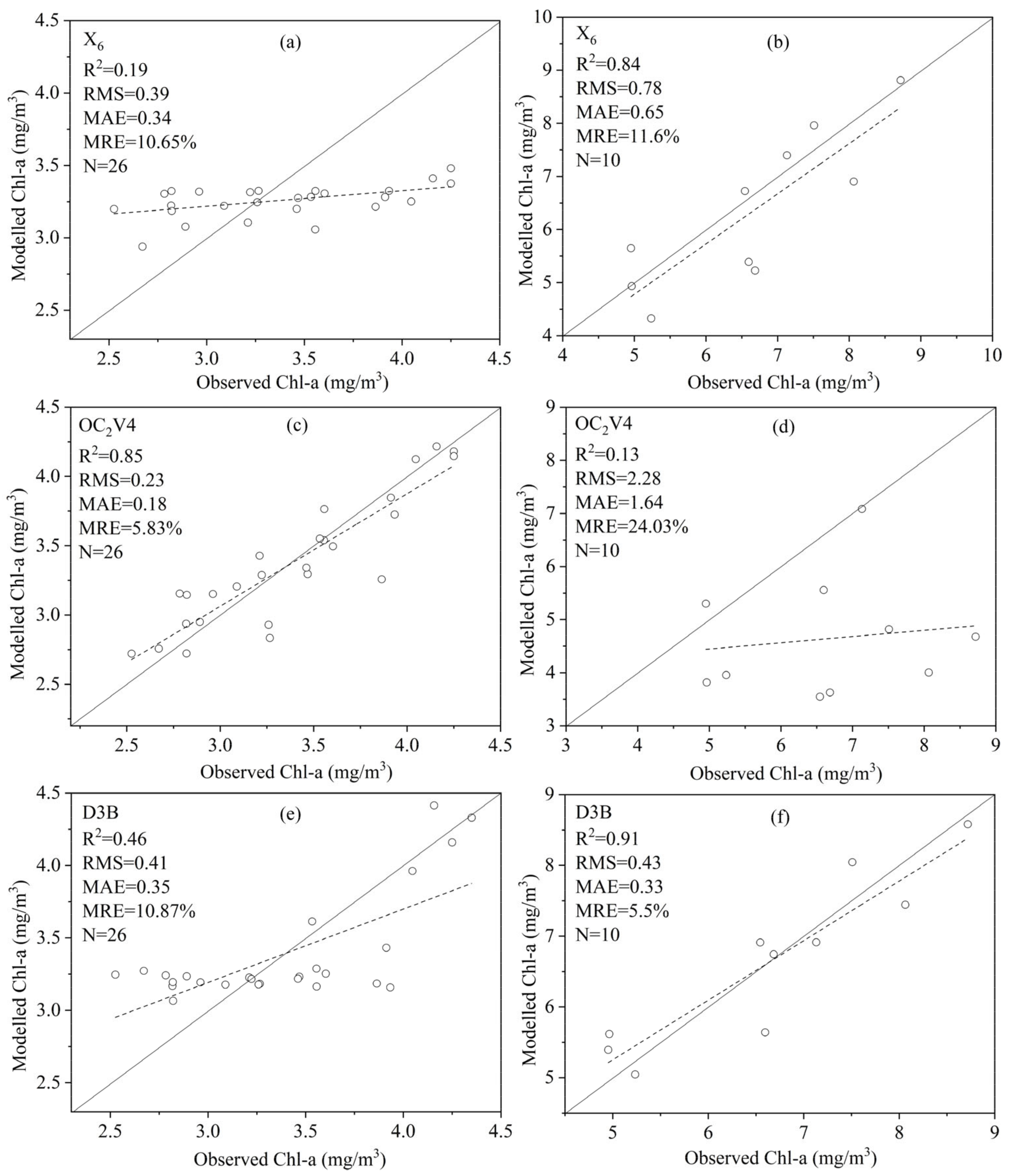
4.1. Comparison of Model Accuracy

Through comparisons of the predicted and measured chl-a concentrations for each verification sample, we can observe that there was a good agreement between these two values (RMSE = 0.51 mg/m³, MAE = 0.40 mg/m³, MRE = 9.10%) (Figure 11). This indicates the feasibility of the piecewise algorithm.

We utilized the piecewise algorithm OC2-D3B to estimate the chl-a concentration for the whole dataset, and then compared the results with those derived from the spectral index model X₆, empirical model OC2V4 and semi-analytical algorithm D3B (Figure 12). It was obvious that the modelled chl-a concentrations from X₆ and D3B algorithms were more scattered in the range of low chl-a compared to measured values. Although the OC2V4 algorithm performed well in the low chl-a concentration, it overestimated the chl-a concentration in the high range. In total, the piecewise algorithms OC2-D3B had better predictability, with a determinant coefficient of 0.96, RMSE of 0.32 mg/m³, MAE of 0.24 mg/m³, and MRE = 5.71%. The experiments in this study demonstrated that the piecewise algorithm would perform better than the individual model.

4.2. Influencing Factors of Chl-a Concentration Change

From Section 4.2, we can observe that the chl-a concentration showed apparent seasonal change patterns. As the study area was located in a high mountain area, it suffered less human disturbance. Therefore, in the following analyses of the controls on chl-a concentration, we attached importance to meteorological factors. Along with the observation data from Bayanbulak meteorological station, we analyzed the influence of three meteorological factors on the changes in chl-a concentration in water bodies, including mean monthly temperature, monthly precipitation and mean monthly sunshine hours from 2016 to 2019. As meteorological factors have a delayed effect on phytoplankton in water, we also analyzed the influence of meteorological factors in the previous month on water bodies’ chl-a concentration. The results revealed that the lag effect of meteorological factors on the chl-a concentration was not enormous in this study area. Consequently, we only discussed the effect of meteorological factors on the chl-a concentration in the corresponding month.

The climate in the study area was characterized by simultaneous rain and hot weather, with obvious seasonal changes. High temperatures and large amounts of rain occur in the summer and low temperatures and less precipitation in winter (Figure 13a,c). The monthly sunshine duration shows complex patterns (Figure 13). We can observe that the changes in chl-a concentration in the water are more consistent with the changing trends of temperature and precipitation. Chl-a concentration reached the highest in summer and the lowest in winter. However, the precipitation was more concentrated within the three months of summer, and the precipitation in other months was low and stable. The relationship between meteorological factors and chl-a concentration (Figure 13b,d,f) suggest that temperature had a higher correlation with chl-a and temperature than precipitation. The correlation coefficient between mean monthly sunshine duration was only 0.38, which indicated that the chl-a concentration of water bodies was probably dominated by temperature and precipitation, and the temperature control is more prominent. This implied that vegetation growth was mainly controlled by temperature and precipitation at high altitudes.

5. Conclusions

Based on the water samples and field-measured spectral information, we performed a comprehensive comparison of the traditional models and our spectral index models. To enhance the prediction accuracy, we finally divided the waters into two groups and built a piecewise algorithm to map the chl-a concentration in the Bayanbulak basin. The findings of this study were as follows.

(1)

Although spectral normalization can distinctly eliminate environmental noise and enhance the correlation between remote-sensing reflectance and chl-a concentration, the models based on spectral normalization did not have a higher performance that the models based on the initially calculated reflectance. This means that the original reflectance could be used to build chl-a models.

(2)

According to the performance of various algorithms after optimization, it is difficult to capture the total change in chl-a concentration using only a single algorithm in water bodies with complex conditions. Although some semi-analytical algorithms, such as G2B, D3B and L4B, had higher accuracy for all types of water bodies, with an average relative error within 20%, their prediction accuracy in water bodies with a low chl-a concentration (≤4.50 mg/m³) was obviously lower than in water bodies with high chl-a concentration. Therefore, a more reliable framework is needed to improve the modelling results.

(3)

The spectral sensitivity analyses showed that the water bodies could be divided into two types (>4.50 mg/m³ and ≤4.50 mg/m³) when the three-band reflectance variable D3B was −0.051. Finally, we constructed an integrated piecewise model to more accurately map chl-a concentration. The modelling results indicated that our piecewise model has a better performance in all types of water bodies (R2 = 0.96, RMSE = 0.32 mg/m³, MAE = 0.24 mg/m³, MRE = 5.71%).

(4)

The chl-a concentration in our study area had a seasonal pattern. The concentration in summer is the highest, followed by spring and autumn, and the lowest in winter. The chl-a concentration in small ponds and riparian wetlands was higher than that in rivers. The correlation between meteorological variables showed that temperature was probably the main driver for variations in chl-a concentration.

References

1. Babin, M.; Morel, A.; Gentili, B. Remote sensing of sea surface Sun-induced chlorophyll fluorescence: Consequences of natural variations in the optical characteristics of phytoplankton and the quantum yield of chlorophyll a fluorescence. Int. J. Remote Sens. 1996, 17, 2417–2448. [Google Scholar] [CrossRef]
2. O’Reilly, J.E.; Maritorena, S.; Mitchell, B.G.; Siegel, D.A.; Carder, K.L.; Garver, S.A.; Kahru, M.; McClain, C. Ocean color chlorophyll algorithms for SeaWiFS. J. Geophys. Res. Ocean. 1998, 103, 24937–24953. [Google Scholar] [CrossRef] [Green Version]
3. Ali, K.A.; Ortiz, J.; Bonini, N.; Shuman, M.; Sydow, C. Application of Aqua MODIS sensor data for estimating chlorophyll a in the turbid Case 2 waters of Lake Erie using bio-optical models. GISci. Remote Sens. 2016, 53, 483–505. [Google Scholar] [CrossRef]
4. Watanabe, F.S.; Alcântara, E.; Rodrigues, T.W.; Imai, N.N.; Barbosa, C.C.; Rotta, L.H. Estimation of Chl-a Concentration and the Trophic State of the Barra Bonita Hydroelectric Reservoir Using OLI/Landsat-8 Images. Int. J. Environ. Res. Public Health 2015, 12, 10391–10417. [Google Scholar] [CrossRef] [Green Version]
5. Gurlin, D.; Gitelson, A.A.; Moses, W.J. Remote estimation of chl-a concentration in turbid productive waters—Return to a simple two-band NIR-red model? Remote Sens. Environ. 2011, 115, 3479–3490. [Google Scholar] [CrossRef]
6. Smith, M.E.; Lain, L.R.; Bernard, S. An optimized Chlorophyll a switching algorithm for MERIS and OLCI in phytoplankton-dominated waters. Remote Sens. Environ. 2018, 215, 217–227. [Google Scholar] [CrossRef]
7. Tassan, S. Local Algorithms Using Seawifs Data for the Retrieval of Phytoplankton, Pigments, Suspended Sediment, and Yellow Substance in Coastal Waters. Appl. Opt. 1994, 33, 2369–2378. [Google Scholar] [CrossRef]
8. Koponen, S.; Attila, J.; Pulliainen, J.; Kallio, K.; Pyhalahti, T.; Lindfors, A.; Rasmus, K.; Hallikainen, M. A case study of airborne and satellite remote sensing of a spring bloom event in the Gulf of Finland. Cont. Shelf Res. 2007, 27, 228–244. [Google Scholar] [CrossRef]
9. Le, C.F.; Hu, C.M.; Cannizzaro, J.; English, D.; Muller-Karger, F.; Lee, Z. Evaluation of chl-a remote sensing algorithms for an optically complex estuary. Remote Sens. Environ. 2013, 129, 75–89. [Google Scholar] [CrossRef]
10. Zhang, Y.; Shi, K.; Cao, Z.; Lai, L.; Geng, J.; Yu, K.; Zhan, P.; Liu, Z. Effects of satellite temporal resolutions on the remote derivation of trends in phytoplankton blooms in inland waters. ISPRS J. Photogramm. Remote Sens. 2022, 191, 188–202. [Google Scholar] [CrossRef]
11. Wenxiang, D.; Caiyun, Z.; Shaoping, S.; Xueding, L. Optimization of deep learning model for coastal chlorophyll a dynamic forecast. Ecol. Model. 2022, 467, 109913. [Google Scholar] [CrossRef]
12. Tong, Y.; Feng, L.; Zhao, D.; Xu, W.; Zheng, C. Remote sensing of chl-a concentrations in coastal oceans of the Greater Bay Area in China: Algorithm development and long-term changes. Int. J. Appl. Earth Obs. Geoinf. 2022, 112, 102922. [Google Scholar] [CrossRef]
13. Qin, J.; Meng, Z.; Xu, W.; Li, B.; Cheng, X.; Murtugudde, R. Modulation of the Intraseasonal Chlorophyll-a Concentration in the Tropical Indian Ocean by the Central Indian Ocean Mode. Geophys. Res. Lett. 2022, 49, e2022GL097802. [Google Scholar] [CrossRef]
14. Liu, H.; He, B.; Zhou, Y.; Kutser, T.; Toming, K.; Feng, Q.; Yang, X.; Fu, C.; Yang, F.; Li, W.; et al. Trophic state assessment of optically diverse lakes using Sentinel-3-derived trophic level index. Int. J. Appl. Earth Obs. Geoinf. 2022, 114, 103026. [Google Scholar] [CrossRef]
15. Legleiter, C.J.; King, T.V.; Carpenter, K.D.; Hall, N.C.; Mumford, A.C.; Slonecker, T.; Graham, J.L.; Stengel, V.G.; Simon, N.; Rosen, B.H. Spectral mixture analysis for surveillance of harmful algal blooms (SMASH): A field-, laboratory-, and satellite-based approach to identifying cyanobacteria genera from remotely sensed data. Remote Sens. Environ. 2022, 279, 113089. [Google Scholar] [CrossRef]
16. Kayastha, P.; Dzialowski, A.R.; Stoodley, S.H.; Wagner, K.L.; Mansaray, A.S. Effect of Time Window on Satellite and Ground-Based Data for Estimating Chl-a in Reservoirs. Remote Sens. 2022, 14, 846. [Google Scholar] [CrossRef]
17. Hu, M.; Ma, R.; Xiong, J.; Wang, M.; Cao, Z.; Xue, K. Eutrophication state in the Eastern China based on Landsat 35-year observations. Remote Sens. Environ. 2022, 277, 113057. [Google Scholar] [CrossRef]
18. Mehrtens, H.; Martin, T. Remote sensing of oligotrophic waters: Model divergence at low chlorophyll concentrations. Appl. Opt. 2002, 41, 7058–7067. [Google Scholar] [CrossRef] [Green Version]
19. Zhang, K.X.; Li, W.; Eide, H.; Stamnes, K. A bio-optical model suitable for use in forward and inverse coupled atmosphere-ocean radiative transfer models. J. Quant. Spectrosc. Radiat. Transf. 2007, 103, 411–423. [Google Scholar] [CrossRef]
20. Cao, Y.N.; Li, X.H.; Ma, S.D.; Ai, J.Y.; Zhu, H.X. Urban Water Absorbance to Predict Chlorophyll a and Turbidity. Aer. Adv. Eng. Res. 2018, 174, 165–172. [Google Scholar] [CrossRef]
21. Yussof, F.N.; Maan, N.; Reba, M.N.M. LSTM Networks to Improve the Prediction of Harmful Algal Blooms in the West Coast of Sabah. Int. J. Environ. Res. Public Health 2021, 18, 7650. [Google Scholar] [CrossRef] [PubMed]
22. Gitelson, A.; Keydan, G.; Shishkin, V. Inland waters quality assessment from satellite data in visible range of the spectrum. Sov. Remote Sens. 1985, 6, 28–36. [Google Scholar]
23. Dall’Olmo, G.; Gitelson, A.A. Effect of bio-optical parameter variability and uncertainties in reflectance measurements on the remote estimation of chl-a concentration in turbid productive waters: Modeling results. Appl. Opt. 2006, 45, 3577–3592. [Google Scholar] [CrossRef] [PubMed] [Green Version]
24. Tang, C.; Wu, Y.; Huang, J. Band Selection of Hyperspectral Chl-a Concentration Inversion Based on Parallel Ant Colony Algorithm. Appl. Mech. Mater. 2014, 675–677, 1158–1162. [Google Scholar] [CrossRef]
25. Dall’Olmo, G.; Gitelson, A.A. Effect of bio-optical parameter variability on the remote estimation of chl-a concentration in turbid productive waters: Experimental results. Appl. Opt. 2005, 44, 412–422. [Google Scholar] [CrossRef] [Green Version]
26. Le, C.F.; Li, Y.M.; Zha, Y.; Sun, D.Y.; Huang, C.C.; Lu, H. A four-band semi-analytical model for estimating chlorophyll a in highly turbid lakes: The case of Taihu Lake, China. Remote Sens. Environ. 2009, 113, 1175–1182. [Google Scholar] [CrossRef]
27. El-Alem, A.; Chokmani, K.; Laurion, I.; El-Adlouni, S.E. Comparative Analysis of Four Models to Estimate Chl-a Concentration in Case-2 Waters Using MODerate Resolution Imaging Spectroradiometer (MODIS) Imagery. Remote Sens. 2012, 4, 2373–2400. [Google Scholar] [CrossRef] [Green Version]
28. Gower, J.F.R.; Doerffer, R.; Borstad, G.A. Interpretation of the 685nm peak in water-leaving radiance spectra in terms of fluorescence, absorption and scattering, and its observation by MERIS. Int. J. Remote Sens. 2010, 20, 1771–1786. [Google Scholar] [CrossRef]
29. Gower, J.; King, S.; Borstad, G.; Brown, L. Detection of intense plankton blooms using the 709 nm band of the MERIS imaging spectrometer. Int. J. Remote Sens. 2005, 26, 2005–2012. [Google Scholar] [CrossRef]
30. Shen, F.; Zhou, Y.X.; Li, D.J.; Zhu, W.J.; Salama, M.S. Medium resolution imaging spectrometer (MERIS) estimation of chl-a concentration in the turbid sediment-laden waters of the Changjiang (Yangtze) Estuary. Int. J. Remote Sens. 2010, 31, 4635–4650. [Google Scholar] [CrossRef]
31. Woo Kim, Y.; Kim, T.; Shin, J.; Lee, D.-S.; Park, Y.-S.; Kim, Y.; Cha, Y. Validity evaluation of a machine-learning model for chlorophyll a retrieval using Sentinel-2 from inland and coastal waters. Ecol. Indic. 2022, 137, 108737. [Google Scholar] [CrossRef]
32. Li, Z.; Yang, W.; Matsushita, B.; Kondoh, A. Remote estimation of phytoplankton primary production in clear to turbid waters by integrating a semi-analytical model with a machine learning algorithm. Remote Sens. Environ. 2022, 275, 113027. [Google Scholar] [CrossRef]
33. Chusnah, W.N.; Chu, H.-J. Estimating chl-a concentrations in tropical reservoirs from band-ratio machine learning models. Remote Sens. Appl. Soc. Environ. 2022, 25, 100678. [Google Scholar] [CrossRef]
34. Cao, Z.; Ma, R.; Liu, M.; Duan, H.; Xiao, Q.; Xue, K.; Shen, M. Harmonized Chl-a Retrievals in Inland Lakes From Landsat-8/9 and Sentinel 2A/B Virtual Constellation Through Machine Learning. IEEE Trans. Geosci. Remote Sens. 2022, 60, 1–16. [Google Scholar] [CrossRef]
35. Asim, M.; Brekke, C.; Mahmood, A.; Eltoft, T.; Reigstad, M. Improving Chl-a Estimation From Sentinel-2 (MSI) in the Barents Sea Using Machine Learning. IEEE J. Stars 2021, 14, 5529–5549. [Google Scholar] [CrossRef]
36. Pahlevan, N.; Smith, B.; Schalles, J.; Binding, C.; Cao, Z.; Ma, R.; Alikas, K.; Kangro, K.; Gurlin, D.; Hà, N.; et al. Seamless retrievals of chl-a from Sentinel-2 (MSI) and Sentinel-3 (OLCI) in inland and coastal waters: A machine-learning approach. Remote Sens. Environ. 2020, 240, 111604. [Google Scholar] [CrossRef]
37. Dekker, A.G.; Brando, V.E.; Anstee, J.M. Retrospective seagrass change detection in a shallow coastal tidal Australian lake. Remote Sens. Environ. 2005, 97, 415–433. [Google Scholar] [CrossRef]
38. Gons, H.J.; Auer, M.T.; Effler, S.W. MERIS satellite chlorophyll mapping of oligotrophic and eutrophic waters in the Laurentian Great Lakes. Remote Sens. Environ. 2008, 112, 4098–4106. [Google Scholar] [CrossRef]
39. Matsushita, B.; Yang, W.; Yu, G.L.; Oyama, Y.; Yoshimura, K.; Fukushima, T. A hybrid algorithm for estimating the chl-a concentration across different trophic states in Asian inland waters. Isprs J. Photogramm. Remote Sens. 2015, 102, 28–37. [Google Scholar] [CrossRef] [Green Version]
40. Zhang, F.F.; Li, J.S.; Shen, Q.; Zhang, B.; Wu, C.Q.; Wu, Y.F.; Wang, G.L.; Wang, S.L.; Lu, Z.Y. Algorithms and Schemes for Chlorophyll a Estimation by Remote Sensing and Optical Classification for Turbid Lake Taihu, China. IEEE J. Stars 2015, 8, 350–364. [Google Scholar] [CrossRef]
41. Odermatt, D.; Danne, O.; Philipson, P.; Brockmann, C. Diversity II water quality parameters from ENVISAT (2002-2012): A new global information source for lakes. Earth Syst. Sci. Data 2018, 10, 1527–1549. [Google Scholar] [CrossRef]
42. Binding, C.E.; Greenberg, T.A.; Bukata, R.P. The MERIS Maximum Chlorophyll Index; its merits and limitations for inland water algal bloom monitoring. J. Great Lakes Res. 2013, 39, 100–107. [Google Scholar] [CrossRef]
43. Gilerson, A.A.; Gitelson, A.A.; Zhou, J.; Gurlin, D.; Moses, W.; Ioannou, I.; Ahmed, S.A. Algorithms for remote estimation of chl-a in coastal and inland waters using red and near infrared bands. Opt. Express 2010, 18, 24109–24125. [Google Scholar] [CrossRef] [PubMed] [Green Version]
44. Gons, H.J.; Rijkeboer, M.; Ruddick, K.G. A chlorophyll-retrieval algorithm for satellite imagery (Medium Resolution Imaging Spectrometer) of inland and coastal waters. J. Plankton Res. 2002, 24, 947–951. [Google Scholar] [CrossRef] [Green Version]
45. Xu, X.; Wang, X.; Zhu, X.; Jia, H.; Han, D. Landscape Pattern Changes in Alpine Wetland of Bayanbulak Swan Lake during 1996-2015. J. Nat. Resour. 2018, 33, 1897–1911. [Google Scholar] [CrossRef]
46. Carlson, R.E. Estimating trophic state. LakeLine 2007, 27, 25–28. [Google Scholar]
47. Shen, M.; Wang, S.; Li, Y.; Tang, M.; Ma, Y. Pattern of Turbidity Change in the Middle Reaches of the Yarlung Zangbo River, Southern Tibetan Plateau, from 2007 to 2017. Remote Sens. 2021, 13, 182. [Google Scholar] [CrossRef]
48. Knaeps, E.; Doxaran, D.; Dogliotti, A.; Nechad, B.; Ruddick, K.; Raymaekers, D.; Sterckx, S. The SeaSWIR dataset. Earth Syst. Sci. Data 2018, 10, 1439–1449. [Google Scholar] [CrossRef] [Green Version]
49. Gitelson, A.A.; Gurlin, D.; Moses, W.J.; Barrow, T. A bio-optical algorithm for the remote estimation of the chl-a concentration in case 2 waters. Environ. Res. Lett. 2009, 4, 045003. [Google Scholar] [CrossRef]
50. Qi, L.; Hu, C.M.; Duan, H.T.; Cannizzaro, J.; Ma, R.H. A novel MERIS algorithm to derive cyanobacterial phycocyanin pigment concentrations in a eutrophic lake: Theoretical basis and practical considerations. Remote Sens. Environ. 2014, 154, 298–317. [Google Scholar] [CrossRef]
51. Main-Knorn, M.; Pflug, B.; Debaecker, V.; Louis, J. Calibration and Validation Plan for the L2A Processor and Products of the Sentinel-2 Mission. Int. Arch. Photogramm. Remote Sens. Spat. Inf. Sci. 2015, XL-7/W3, 1249–1255. [Google Scholar] [CrossRef] [Green Version]
52. Mishra, S.; Mishra, D.R. Normalized difference chlorophyll index: A novel model for remote estimation of chl-a concentration in turbid productive waters. Remote Sens. Environ. 2012, 117, 394–406. [Google Scholar] [CrossRef]
53. Reynolds, C.S.; Descy, J.P.; Padisak, J. Are Phytoplankton Dynamics in Rivers So Different from Those in Shallow Lakes. Hydrobiologia 1994, 289, 1–7. [Google Scholar] [CrossRef]
54. Carneiro, F.M.; Nabout, J.C.; Vieira, L.C.G.; Roland, F.; Bini, L.M. Determinants of chl-a concentration in tropical reservoirs. Hydrobiologia 2014, 740, 89–99. [Google Scholar] [CrossRef]
55. Staehr, P.A.; Baastrup-Spohr, L.; Sand-Jensen, K.; Stedmon, C. Lake metabolism scales with lake morphometry and catchment conditions. Aquat. Sci. 2012, 74, 155–169. [Google Scholar] [CrossRef]
Figure 1. Sampling sites in the Bayanbulak wetland in Xinjiang.
Remotesensing 14 06119 g001
Figure 2. The reflectance spectrum curves of the water surface at the sampling sites (N denotes the number of samples). (a) The in situ water surface reflectance spectrum of sampling sites with chl-a concentration ≤ 4.50 mg/m3; and (b) in situ water surface reflectance spectrum of sampling sites with chl-a concentration >4.50 mg/m3. The spectrum in the red box shows the spectral characteristics caused by chl-a.
Remotesensing 14 06119 g002
Figure 3. Correlation coefficient between single-band remote sensing reflectance and in situ chl-a concentration.
Remotesensing 14 06119 g003
Figure 4. The distribution of correlation coefficient between in situ chl-a and the three specific indexes. (a) correlation coefficient between in situ chl-a and R r s λ 1 R r s λ 2 ; (b) correlation coefficient between in situ chl-a and R r s λ 1 / R r s λ 2 ; and (c) correlation coefficient between in situ chl-a and R r s λ 1 R r s λ 2 / R r s λ 3 + R r s λ 4 .
Remotesensing 14 06119 g004
Figure 5. Correlation between the calculated D3B value and measured chl-a concentration.
Remotesensing 14 06119 g005
Figure 6. The performance metrics of the twelve chl-a concentration retrieval models. (N is the number of samples). (a) All water samples, (b) samples with low chl-a concentration, and (c) samples with high chl-a concentration.
Remotesensing 14 06119 g006
Figure 7. In situ chl-a versus estimated chl-a of X6, OC2V4 and D3B in the two separate chl-a datasets. Figures (a,c,e) showed the results of low chl-a concentration, while figures (b,d,f) showed the results of high chl-a concentration. (N is the number of samples).
Remotesensing 14 06119 g007
Figure 8. Spatial distribution of estimated chl-a using the OC2V4 (a), D3B (b), and OC2-D3B (c).
Remotesensing 14 06119 g008
Figure 9. Estimated chl-a concentration versus in situ measured chl-a concentration (P denotes sample site number).
Remotesensing 14 06119 g009
Figure 10. (a) Temporal variation in mean monthly chl-a concentration in study area from 2016 to 2019, and (b) the seasonal variation of multi-year average chl-a concentration.
Remotesensing 14 06119 g010
Figure 11. Comparison of the estimated (OC2-D3B) and measured chl-a concentrations after cross-validation.
Remotesensing 14 06119 g011
Figure 12. In situ chl-a versus estimated chl-a of X6 (a), OC2V4 (b), D3B (c) and OC2-D3B (d) for all the samples.
Remotesensing 14 06119 g012
Figure 13. The temporal change of chl-a concentration and its controls, including temperature (a), precipitation (c) and sunshine duration (e). The (b,d,f) represent the correlation between chl-a and temperature, precipitation and sunshine duration.
Remotesensing 14 06119 g013