Abstract
Large urban areas are vulnerable to various geological hazards and anthropogenic activities that affect ground stability—a key factor in structural performance, such as buildings and infrastructure, in an inherently expanding context. Time series data from synthetic aperture radar (SAR) satellites make it possible to identify small rates of motion over large areas of the Earth’s surface with high spatial resolution, which is key to detecting high-deformation areas. Santiago de Chile’s metropolitan region comprises a large Andean foothills basin in one of the most seismically active subduction zones worldwide. The Santiago basin and its surroundings are prone to megathrust and shallow crustal earthquakes, landslides, and constant anthropogenic effects, such as the overexploitation of groundwater and land use modification, all of which constantly affect the ground stability. Here, we recorded ground deformations in the Santiago basin using a multi-temporal differential interferometric synthetic aperture radar (DInSAR) from Sentinel 1, obtaining high-resolution ground motion rates between 2018 and 2021. GNSS stations show a constant regional uplift in the metropolitan area (~10 mm/year); meanwhile, DInSAR allows for the identification of areas with anomalous local subsistence (rates < −15 mm/year) and mountain sectors with landslides with unprecedented detail. Ground deformation patterns vary depending on factors such as soil type, basin geometry, and soil/soil heterogeneities. Thus, the areas with high subsidence rates are concentrated in sectors with fine sedimentary cover and a depressing shallow water table as well as in cropping areas with excess water withdrawal. There is no evidence of detectable movement on the San Ramon Fault (the major quaternary fault in the metropolitan area) over the observational period. Our results highlight the mechanical control of the sediment characteristics of the basin and the impact of anthropogenic processes on ground stability. These results are essential to assess the stability of the Santiago basin and contribute to future infrastructure development and hazard management in highly populated areas.
1. Introduction
Santiago basin is the homonymous capital of Chile with more than 7 million inhabitants [1]. Along with a high population density, the capital and its surroundings comprise the majority of the economic, political, and social activities of the country. Therefore, knowledge of the geohazards of the territory where the city of Santiago is located is essential for land use planning and sustainable growth. The Santiago forearc basin has been formed in a compressive tectonic environment in which the uplift of the Andes during the Miocene conditions caused the basin development in its eastern flank. The contact between the basin and the Andean Cordillera is formed by reverse faulting (San Ramon Fault). Previous geological/geophysical studies in the Santiago Metropolitan Area aimed at evaluating geohazards have focused on geology and hydrogeology [2,3,4], seismic potential and micro-zoning [5,6], and tectonics [7,8,9,10]. Despite advancement in the knowledge and assessment of geohazards in the Santiago basin, few studies have been carried out to analyze the ground surface stability and deformation of the whole basin. In this sense, this research focuses on studying the ground deformations of the metropolitan area using advanced DInSAR technology and ground deformation time series.
The seismic cycle of megathrust earthquakes is the main driver of ground deformation in subduction zones. This process induces long wavelength deformations with regional vertical patterns that oscillate between uplift and subsidence depending on the stage of the seismic cycle and its distance from the trench [11]. Upper plate faults define a secondary earthquake cycle system that has a direct impact on ground deformation. These faults have a long period of elastic energy accumulation (>1000 years) [12] (much longer than the recurrence of earthquakes in the megathrust), during which they induce a very low magnitude deformation of a few mm/year; this was described by [13] in the Andean region close to those faults. To date, it is unclear under which conditions upper plate faults are reactivated and by which mechanism they interact with the plate interface.
It is difficult to estimate upper plate contribution to the ground deformation due to the lack of observables at broad temporal and spatial scales and the fact that active continental faults can be blind in the sense that their location and recent activity may be unknown. Other natural drivers of subsidence and uplift include glacial isostatic adjustment [14], sediment compaction [15], and seasonal hydrological loading [16]. On the other hand, human-induced processes can cause surface level changes on a smaller spatial scale but with a faster response time. Anthropogenic ground deformations can be associated with the exploitation of groundwater [17,18] and hydrocarbons [19,20,21], which implies subsidence from local to regional scales. Furthermore, much more rapid anthropogenic causes may be related to urbanization, such as building load or removal of materials typically in unconsolidated alluvial deposits, which are linked to surface processes [22,23].
Land surface deformations caused by anthropogenic processes and hydrogeological phenomena, such as the compaction of aquifers, are slower processes that induce low rates of subsidence; therefore, they do not involve situations of immediate risk as their effects are observed after several years. However, over a period of several years, their effects can change the topography of the land surface, causing damage to the population and civil infrastructure. Quantitative evaluation of ground deformation can be performed based on ground instrumentation and traditional measurement techniques (related to topography/geodesy), i.e., leveling and GNSS [24]; however, these are limited in terms of producing high spatial resolution surface displacement maps over wide areas. DInSAR technology is an alternative solution totally assimilable to terrestrial monitoring [25]. Ground deformation monitoring with DInSAR takes advantage of the amount of available data that is acquired more frequently and accurately at low cost, and such characteristics make it an attractive source of information [26]. One of the main attractions of satellite-based DInSAR is its ability to cover areas at a systematic and continuous rate remotely, which makes it suitable as a structural monitoring and control tool as we can detect near-vertical deformations in the structures along the LOS (line of sight). In recent years, the DInSAR time-series technique has emerged as an essential tool for measuring slow surface displacement [27]. This technology has been widely exploited in a wide variety of contexts such as seismic deformation [28,29], volcanic and landslide monitoring [30,31,32], infrastructure stability studies [26,33,34], and water overexploitation surface effects [35,36,37].
DInSAR technology is essentially based on two approaches associated with the selection of coherent pixels: the Persistent Scatterers (PS) technique, developed by Ferretti et al. [38], and the SBAS (Small BAseline Subset), developed by Bernardino et al. [39]. These processing techniques involve multiple time-dependent acquisitions to provide characteristic displacement patterns of surface motion over a period of time, thus providing measurement of surface uplift or subsidence to identify cyclical patterns (due to seasonal variations), trends, and anomalous variations. Such techniques can be applied to collect time series of movements of the earth’s surface over wide areas with millimeter precision [40,41,42]. The evolution of DInSAR techniques observed in recent years is mainly related to the development of advanced computational algorithms [43]. However, it is also the result of greater possibilities for the acquisition of radar images by satellite missions and their high review frequency of 6 to 12 days for the entire world. Of particular note is the European Space Agency (ESA) Copernicus mission material that we use in this work, consisting of two twin SAR satellites, Sentinel 1A and Sentinel 1B [44].
This research quantifies the temporal evolution of ground motion through the analysis of the SAR interferometry with geophysical and geological data characterizing the features of the Santiago basin. The methodology of this study uses DInSAR differential interferometry with ground-based information. We use a C-band Sentinel 1 to process multiple SAR images with the P-SBAS (Parallel Small BAseline Subset) algorithm [43,45,46], an evolution of the traditional SBAS (Small BAseline Subset) method [39] developed by the CNR—IREA (Institute for Electromagnetic Sensing of the Environment). For the processing of SAR images, we used the iCloud platform (GEP) [47,48,49,50]. The results presented here provide new information that identifies the stability of the city of Santiago and constrains subsistence-inducing factors, such as hydrogeological phenomena, due to the overexploitation of water and stability of slopes in areas susceptible to landslides.
2. Present Day Regional Deformation and Geological Setting
The subduction of the Nazca Plate beneath the South American Plate controls the seismic cycle of large earthquakes and contributes to the permanent deformation that shapes the main morphological features on the Chilean margin. The Santiago basin is located at about 520 m above sea level at the piedmont of the Andean Precordillera, which reaches over 4000 m in altitude (Figure 1b). Santiago lies in the central segment of the Chilean subduction zone, between the rupture zones of the Maule 2010 [51] and Illapel 2015 [52] earthquakes. This segment is considered a seismic gap, in which the last major earthquake that ruptured the entire segment, both along and across the megathrust, was in 1730 [53]. Velocities derived from GNSS observations between 2018 and 2021 show typical interseismic deformation patterns (Figure 1). In this period, Central Chile moved northeastward with magnitudes of ~20 mm/year near the coast, decreasing to ~10 mm/year in Santiago (Figure 1c). Vertical velocities show subsidence near the coastline, suggesting that the offshore megathrust zone is locked, as previous studies have shown [54]. The Santiago basin and its surroundings show a regional uplift trend of about 10 mm/year. The velocity field shows no horizontal or vertical gradients near the San Ramon fault, so no activity or movement related to this fault are observed.
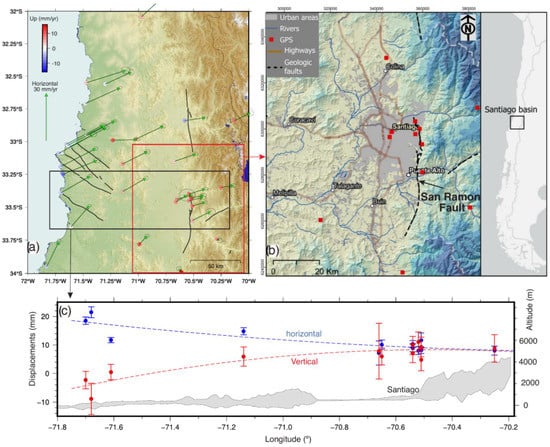
Figure 1.
(a) Central Chile region showing the GNSS velocity field and traces of active faults (from Maldonado et al. [55]). The red and blue rectangles indicate the corresponding areas of Figures (b,c), respectively. (b) Geographical location of the metropolitan area of Santiago de Chile, ALOS DEM 30 mts, was used as background. (c) Cross-section of horizontal (blue) and vertical (red) velocities derived from GNSS data (from Donoso et al. [56]). A swath profile of the topography is shown in gray.
The Santiago forearc basin developed during successive tectonic events divided into two stages. The first stage of the Middle Eocene to the Oligocene-early Miocene was characterized by an extensional setting, which created depocenters where the Abanico Formation accumulated [57]. A second stage of compression linked to an increase in the rate of plate convergence velocity [58] dominated the evolution of the Abanico Basin until the Miocene. This produced the change to a compressive regime, with a partial tectonic inversion of the Abanico basin from the late Oligocene to early Miocene, inverting the larger NS normal fault systems generated in the first stage [59,60,61,62,63]. The Coastal Cordillera is located at the western flank of the basin, which is composed of Jurassic to Late Cretaceous volcanic and sedimentary sequences and Jurassic to Cretaceous intrusive rocks. At the eastern border of the basin, the foothill of the Andean Cordillera corresponds to a thrust deformation front that causes the uplift of the Andean Cordillera [64] and at the same time, the erosional process that provides the sedimentary supply for the basin infill.
Given the high-energy mountain erosional process, most of the basin deposits correspond to coarse gravel material (Figure 2a); however, in the northern part of the basin, some fine sediments associated with low-energy lacustrine-type deposits are still observed (Figure 2b). Based on gravity measurements constrained by geological observations at wells, it has been possible to estimate the thickness of the sedimentary cover as being in the range of 100–400 m with an irregular morphology [3]. The role of the eastern deformation front, whose westernmost branch correspond to the San Ramon Fault System (SRFS), has been a source of large scientific debate in terms of its relevance as a seismic hazard source [7,8,9,10,65]; maximum seismic events and recurrence times are among the most relevant unresolved questions. Finally, the basin water table is controlled by surface topography (tilted to the west), asymmetric basin (shallowing to the west), the overexploitation of the water resource, and the limited recharge due to a prolonged drought [66]. Rates of water table descent in the last 10 years range between 1–0.3 m/year, probably due to a combined effect of the lack of recharge and overexploitation. These first order geological characteristics of the Santiago Basin are used in this study to explain the surface deformation derived from the DInSAR observations.
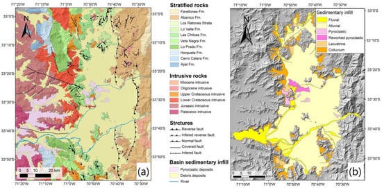
Figure 2.
(a) Geological map and (b) Sediment map of Santiago Basin (From Yanez et al. [3]).
3. Materials and Methods
The methodology describes the study of the deformation in the Santiago Metropolitan Area during an observation period of 3 years (2018–2021), using the multitemporal differential interferometry technique (DInSAR). The data obtained with the interferometric radar is complemented by a contextualization of the deformation obtained with the GNSS stations and, furthermore, by available geological and hydrogeological studies to propose a plausible interpretation of the observed anomalous domains. We integrate the results of the DInSAR analysis with the geological background, which allows us to describe the processes responsible for the detected anomalies. Thus, we present detailed high-resolution maps of the entire Santiago Basin, where records of ground deformation were previously lacking. In addition, the long time series with DInSAR and the high spatial density of PSI (Persistent Scattering Interferometry) can undoubtedly contribute to urban planning in Chile.
The main phases of the workflow include: (1) SAR image processing to generate interferograms, (2) SAR time series analysis using (3) vertical and slope velocity estimation in the post-processing, (4) overlaying with geological and hydrogeological information, and Digital Elevation Models (DTM) (5) to interpret the processes responsible for the anomalies detected.
3.1. Data Set
We have used 204 interferometric C-band VV polarized wide fringe (IW) SAR scenes acquired by the Copernicus Sentinel-1 mission [67] along ascending and descending orbits (Table 1). The review time for each stack is 12 days, with a resolution of 5 (terrestrial range) by 20 (azimuth) and angles of incidence (θ) of 31 to 46°. We use the IW-2 swath width and bursts 2–4 to cover the Santiago Basin area of interest. Through the GEP platform, we retrieved updated SAR images from the ESA Open Access Hub repositories as a Single Look Complex (SLC) interferometric product [68]. The advantages of Sentinel-1 come from its wide range coverage (250 km swath in wide interferometric mode) and sufficient spatial resolution for large areas (90 m × 90 m range vs. azimuth, for this case). The Wide Interferometric Fringe (IW) acquisition mode is based on the ScanSAR terrain observation mode and the use of interferometric fringes with progressive scans (TOPS).

Table 1.
Data set including the main features of Sentinel 1.
3.2. Data Processing
The processing has been based on the Advanced Earth Sciences Cluster operated by Terrafirma with a duration of approximately 48 h of run-time. We adopt SAR processing running on ESA’s next-generation GEP iCloud platform, “CNR-IREA P-SBAS Sentinel-1 on-demand processing” service v.1.0.0, implemented in the computer-based operating environment ESA GRID [43]. The processing approach is based on the SBAS technique [39], applied along the descending orbit of Sentinel-1B (C-band SAR sensor wavelength = 5.6 cm). The algorithm was adapted to run efficiently on high-performance distributed computing and configured for Sentinel-1 IW TOPS data processing [45].
The main processing steps of the SBAS method [39] consist of the generation of differential interferograms from the SAR image pairs formed with a small orbital separation (spatial baseline) to reduce spatial decorrelation and topographic effects. The Shuttle Radar Topography Mission (SRTM) [69] with 1 arcsecond DEM from NASA (~30 m pixel size) and precise orbits from the European Space Agency (ESA) were used for the joint registration and removal of the topographic signal from the interferometric phase in each of the computational interferograms.
Each SLC data stack was co-recorded at the single burst level, ensuring very high co-registration accuracy (on the order of 1/1000 azimuth pixel size), as required for TOPS data due to the great Doppler centroid along the path variations [70]. The temporal consistency and the threshold of the minimum temporal consistency was set at 0.85. Atmospheric phase components were identified and removed. The control point for the P-SBAS processing was established in the same place in the city of Santiago center with coordinates lat: −62.555, log: −35.172, where the annual LOS velocity values were taken, and the time series were referenced accordingly. The use of a common reference point allowed internal calibration of the two output data sets.
3.3. Post-Processing
With the persistent scatterer interferometry (PSI) dataset, we project the vertical velocity and the velocity along the steepest slope estimates using the principles mentioned below.
The estimates of the vertical velocity component have been made with the combined ascending and descending data sets to obtain the vertical displacement . A 90-m square element network was used to resample the point data sets on a regular grid and link the output data sets into a single layer. Both P-SBAS outputs (ascending and descending) were available at the same location, i; the combination was achieved under the assumption of negligible north−south velocity, = 0. This assumption is typically used in DInSAR studies to consider the relatively poor visibility of the north−south horizontal motions that the LOS sensor can achieve [68]. The horizontal E−W displacement components in the Santiago basin region are much lower than the vertical ones; therefore, they were not considered for our case.
Given the known values of the deformation velocity LOS in the ascending () and descending () mode at each location i, the is estimated as follows:
The estimation of velocity deformation along the Steepest Slope Direction defines zones potentially affected by landslides, considering the geomorphological principle upon which deformation is more likely to occur along the slope direction [71]. This is true for translational landslides and other types of movements present in some sectors of the study area, such as the debris flow. Under the assumption that the displacements occur along the direction of the steepest slope, they were projected considering the local values of slope (β) and aspect (γ) from the DTM ALOS PALSAR 30 mts. These data were used to identify the orientation of the steepest slope of the Andes mountain range, where the value represents the conversion factor of the LOS to slope values. , , and are the directional cosines of the LOS and the SLOPE vectors in the east, north, and zenith directions, respectively, and they are defined as follows:
. The velocity along such direction () was then estimated as follows (Cigna et al. [72]):
4. Results and Discussion
GNSS velocities allow us to characterize the regional deformation field in Central Chile. These data show widespread uplift in and around the Santiago Basin. However, the distribution of GNSS stations does not allow the identification of local uplift and subsidence. Hence, DInSAR data are an excellent complement to improve the spatial resolution of land-level changes and explore features of local deformation. The results of the SAR image processing provide detailed information to represent the phenomenon of ground deformation over the study area. The data set contains the Persistent Scatterers Interferometry (PSI) data, where each PSI contains a LOS displacement time series; average LOS velocity; temporal Coherence > 0.85; average elevation of the scatterer (topography); and the unit vectors that are the directional cosines of the LOS in the east (E), north (N), and zenith (U) directions, respectively. These were then used for the vertical and velocity along the steepest slope projections in the post-processing phase.
The data set output format is a CSV file, according to the specifications of the European System of Plate Observation—Phase Implementation (EPOS—IP), where the metadata corresponding to the LOS velocity in raster (.png) and Google Earth (.kml) are standardized. With these contents, we georeferenced GIS-based cartography (WGS84—UTM zone 19S) to represent and provide evidence for the phenomenon of deformation over the study area. Our results present an overview of the ground deformation for both orbits, selecting the PSI of the Santiago Basin area and identifying the local subsidence areas. In addition, we present the displacement map of the estimated vertical components based on the projections of the ascending and descending LOS and the displacement along the maximum slope in the Andean Cordillera area, resampling the LOS velocity.
4.1. PSI Measurement and Classifications
PSI measurements from 2018–2021 have been classified according to deformation velocity rate (mm/year), with a continuous color scale that varies from dark green to dark red. Negative velocity values indicate motion away from the satellite sensor (orange to dark red PSI), while positive values indicate motion toward the sensor (light to dark green PSI). Although we have not used the maximum resolution of the Sentinel 1 (IW) images, the PSI are spaced in 90 × 90 grids, the interferometric data deliver a high density of points, reaching 100 PSI/km2 in urban areas and PSI 60 PSI/km2 in rural areas where it is usually covered by more vegetation, which decreases SAR detection. For both cases, we have appointed an optimal data set to represent the phenomenon of deformation in the study area. With the Persistent Scatterer Interferometry (PSI) dataset, we project the vertical velocity and the velocity along the steepest slope estimates using the principles mentioned below.
We obtained the PSI LOS deformation maps for the ascending and descending orbits, covering the entire study area, the Santiago basin, and the western flank of the Andean Mountain range (see Figure 3). An indicator of the compatibility between acquisition geometries is the standard deviation of the mean LOS strain rates, which correspond to 0.47 mm/year and 0.55 mm/year for the ascending and descending orbits, respectively. Given the difference in the area covered by each orbit, the relatively greater number of PSI points in the ascending solution could be explained by the morphology of the area and the angle of incidence on the mountainous cover. Apart from the effect of area coverage, it appears that the total number of PSI targets is comparable. This similarity can be attributed to the common observation period and the ascending and descending data sets. PSI LOS velocities in 2018–2021 ranged from −25.56 to +2.73 cm/year in the ascending dataset and from −28.79 to +3.05 mm/year in the descending dataset (see Table 2).
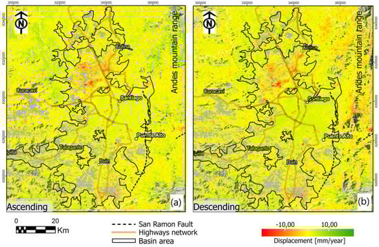
Figure 3.
(a) LOS displacement maps for the study area, (a) Ascending orbits (A18), and (b) Descending orbits (D156), with ALOS DEM 30 mts used as background.
Table 2.
Basic PSI statistical comparison for ascending and descending orbits.
4.2. Deformation Overview and Vertical Displacement
The deformation overview in the Santiago Metropolitan Area, was calculated with the vertical projection using ascending and descending LOS. Thus, we resampled the data considering the similarity of both data sets from both orbits. Vertical velocity component estimates were calculated after combining the two data sets where a 90 square meter grid was used to resample the point data sets on a regular grid and link the output data sets. This single digital layer in SHP format allowed us to create a new vertical deformation map (see Figure 4a).
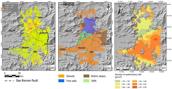
Figure 4.
(a) Vertical displacement maps for study area, (b) Sediment cover map, and (c) Density of sedimentary infill map (modified from Yanez et al. [3]), with ALOS DEM 30 mts used as background.
The median ground stability is represented by the yellow PSI and varies between −4.99–0.00 (mm/year), indicating a general trend of negative velocities that indicate a pervasive subsidence. On top of this general trend, we found two anomalous domains in which the subsidence rate is much larger: a) The northern domain, over a NE elongated surface of more than 500 km2 (Quilicura, Chicureo, and Colina localities), in which subsidence up to −25.00 mm/year is observed (Figure 4a)the southeastern domain, along a more restricted surface of 250 km2 (Paine, Huelquen localities), with subsidence in the order of −15.00 mm/year. The two anomalous domains of relatively large subsidence rates are associated with fine deposits of lacustrine origin in the northern domain and gravel deposits in the southern domain (Figure 4b). However, in terms of the deposit densities, both anomalous domains share the presence of low-density deposits in the southern region, probably associated with the distal disposition with respect to the Maipo River. On the other hand, these two anomalous domains show different soil use throughout the last few decades; while the southeastern domain is still dedicated to two agricultural activities, the northern domain has experienced a rapid transition to urban areas. In Section 4.3 we interpret these anomalous domains in terms of the interaction between soil characteristics and the spatial/time evolution of the groundwater processes in the basin.
Finally, the most stable soils are in Santiago’s center and they are shown in the PSI of green colors with values between 0.99–5.00 (mm/year). For this area, a slight upward trend can be observed and this is probably caused by the tectonic processes that affect the Santiago Basin regionally. For the area near the San Ramon fault, no indication of fault activity was observed in the analyzed time window; however, an uplift caused by the same regional tectonic effects as those in the central area of Santiago is observed.
4.3. Ground Deformations and Time Series
Multi-temporal satellite radar interferometry is based on the analysis of a series of SAR (Synthetic Aperture Radar) images, which, in our case, were acquired in the period between May 2018–May 2021. By selecting the most stable targets in the anomalous areas (PSI > 0.85) that maintain the electromagnetic scattering signature in each image, it is possible to measure ground displacements by exploiting the phase shift (sensor–target distance) and the amplitude of the signal reflected from the ground surface.
The product generated by this multi-interferometric analysis is a cartographic representation of the time series, with a cumulative displacement value of up to −100 (mm) for isolated PSI targets and values of −74–50 (mm) for homogeneous areas (see Figure 5). The records of interferometric data for both orbits allowed us to know the temporal evolution of the deformation phenomenon in the study area and build the time series in the anomalous areas. For this we have selected 8 pixels of the study area, numbered from 1–8, where each one is assigned the name of the locality where the deformation phenomenon occurs.
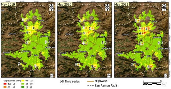
Figure 5.
Map of cumulative displacements and temporal evolution (a) Recorded in May 2019 (b), Recorded in May 2020, and (c) Recorded in May 2021, with Maxar image (source Esri) used as background. Numbers in each panel label the localities in which the deformation time series response is described in the text of Section 4.3.
Deformation time series represent the most advanced DInSAR product. They provide the history of the deformations during the observed period, which is fundamental to represent and study the ground deformation in the study area and its correlation with the inducing factors. To properly use, interpret, and exploit deformation time series, it is important to consider that they can be affected by geometric and atmospheric distortions. In fact, they contain an estimate of the deformation for each acquisition (SAR image), so they are particularly sensitive to phase noise [40].
Following the results in the deformation area (Pixels 1–8), we focused on a quantitative analysis, comparing each of the ascending and descending time series, based on the parameters of velocity and R2. We present graphs in Figure 6, which show the time series comparisons of the orbits of the interferometric data developed in the processing phase of the images of Sentinel-1, corresponding to LOS, ascending (blue color), and descending orbits (red color). According to the above results, there is very good agreement between the measurements. However, the difference in the SAR-derived time series 7 and 8 (Figure 6) between the ascending and descending orbits is a consequence of the distances between the pixel’s PSI, which reach up to 100 m so the pixels can detect different local deformations. For the time series 1, 2, 3, 4, and 6, the values of R2 (Figure 6) are close to 1.0 with a good fit; therefore, the results of both orbits are very mutually reliable, indicating a negative displacement trend (subsidence). For time series 5, the values of R2 are close to 0, and this is similar for both orbits, indicating a stable deformation. In time series 7 and 8, the R2 values are also close to 1.0; however, there is a difference due to the distance between the PSI pixels, indicating a trend of seasonal subsidence.
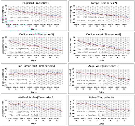
Figure 6.
Time series 1–8 in red ascending orbit and blue descending orbit, located at Polpaico, Lampa, Quilicura nord, Quilicura west, San Ramon fault, Maipu west, Wetland Aculeo, and Paine.
The time series of displacements show values of up to −60 (mm) for the period of May 2018–May 2021 or ~20 mm/year. The greatest deformations are located in the northern area of Santiago, in the towns of Polpaico (Time series 1), Lampa (Time series 1), and Quilicura (Time series 3–4). On the other hand, the area of the San Ramon fault (Time series 5) appears stable and there is no evidence of activity in the fault. In Maipu west (Time series 6), an anthropogenic deformation caused by the increase in urbanization in the area is observed. The wetland “Aculeo” (Time Series 7) is close to the “Aculeo” lake, which has been drying up dramatically [73,74]. Finally, for Paine (Time Series 8), an area of intensive agriculture shows an increase in subsidence in recent years.
4.3.1. Subsidence and Groundwater Spatial and Temporal Evolution
Given the spatial relationship between anomalous deformation, mostly subsidence, soil characteristics, and the known increase of groundwater exploitation, both for agriculture and for human consumption, were explored in this section with the working hypothesis that the main factors that cause the deformation of the Santiago Basin are linked with changes in groundwater flow and static levels.
In order to determine the water table of the Santiago Basin, we include a water table grid produced by DGA (2000) [75] in Figure 7b, which is a compilation of data up until the year 2000. This map shows that the anomalous DInSAR domains (Figure 7a) are located in shallow areas of the water table. In addition to that, and with the aim to validate this water table map while exploring the time evolution of the water table at the same time, we analyzed 48 wells within the area of interest. From these wells we extract time series evolution of the water table at a rate of 2–4 points per year. From this basic data we calculate a trend to have the gradient per year and an average value for the last 10 years. Comparing Figure 7b,c, we conclude that the DGA 2000 map is basically correct and still valid today, with the deeper water table in the central and eastern part of the basin, and the shallower ones in the northern, southern, and western flanks. The majority of the wells show a decrease in its water table, with some of them in excess of 1–2 m/year; however, in the central part of the basin (Quinta Normal), the well shows that the water table indeed becomes shallower (at rates greater than 1.5 m/year). A qualitative comparison between water table evolution and deformation of the surface according to DInSAR show an apparent inconsistency, zones with large water table oscillation show no or minor deformation, i.e., in the central part of the basin. However, a closer look shows that, in general, these areas are associated with zones of deeper water table and coarse soil in the area of high energy of the fluvial system. In order to gain a better understanding of the role of groundwater dynamics in surface deformation, we need to consider some basic concepts of pore elasticity.
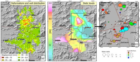
Figure 7.
(a) Ground deformation map and well distribution in white point color, (b) Static level map (modified from DGA 2000), and (c) Piezometric variations maps, with ALOS DEM 30 mts used as background.
According to the pore-elastic model developed by Terzaghi, K. [76] and Biot, M. [77], the variation in effective stress (geostatic stress minus pressure head) is related to changes in the hydraulic head (Δh). Then, if such a stress field is applied over a compressible matrix aquifer, they result in a matrix deformation, including surface deformation (Δu). For a simple one-dimensional compaction model, Terzaghi, K. [76] established a linear relationship between (Δu) and (Δh), where the constant of proportion is the skeletal storage (Sk), such that Δu = Sk ∗ Δh. The main factors that control skeletal storage are the compression index (Cc) and the effective stress and the direct and reverse dependence. Effective stress increases with depth, so larger effects are expected in shallow aquifers. Compressional index depends on the granulometry of the soil: fine soil (i.e., clay and silt) show larger Cc, whereas coarse and more rigid soils (i.e., gravels) show Cc values practically zero, regardless of any other factor.
In the Santiago Basin, the DInSAR show a major subsidence effect in the northern anomalous domain (Figure 7a), in good spatial agreement with the region in which the static level is shallower than 10 m (Figure 7b) and where fine sediments of lacustrine origin are emplaced (Figure 4b in Yanez et al. [3]). The southeastern anomalous domain is also located in a shallow water table region, where gravel sediments show low-density, and thus distal, fine sediments. On the other hand, most of the central and southern part of the basin is dominated by the high-energy gravel material, which is highly rigid, having an almost zero compressional index. In addition to that, the water table in this region shows depths deeper than 50 m (Figure 7b,c). Both factors correctly predict a minor or null surface deformation, as observed in the DInSAR data. The Δu/Δh ratio, which is the skeletal storage in this case, is in the order of 0.01 in the anomalous domains. These values are in good agreement with observations in central Mexico [78], Kumato area, Japan [79], and Tucson Arizona [80].
4.4. Landslide Identification
In recent decades, the metropolitan area of Santiago has experienced sustained growth in urbanization towards the Andes Mountain range, where landslide activity is more frequent. The occurrence of landslides in the front of the mountain and on the slopes of the interior basins and, in particular, debris flows that can reach the alluvial plain are common and represent an increasing risk for populated areas [81,82]. A large debris flow event in 1993 [83,84] is an example of the potential impact of catastrophic landslides in the area. The most common types of landslides in the area are debris flows that occur from the mountain range towards the city, rock falls from steep and fractured slopes, and rock slides [85].
To identify landslides, it is necessary to identify the geomorphological units, because they have different conditions that can define a type of landslide, in addition to the fact that the geomorphological unit is favorable for one type of landslide but not for another. For this reason, we have focused the analysis using the susceptibility map (Figure 8a) to mainly debris and rock flows. We also considered the high coherence of the SAR in highly reflective rocky areas. To compare our PSI interferometric data, we used a landslide susceptibility map [86], which shows areas that have the potential for landslides (see Figure 8a), determined by the correlation of some of the main factors that contribute to landslide generation. The area is affected by the main geometric distortions of shadows, layover and foreshortening, where the differences between the ascending and descending orbits are evident and can be seen in Figure 8b,c.
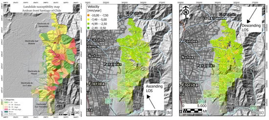
Figure 8.
(a) Landslide susceptibility map (modified from Celis, C. [86]), (b) LOS displacement map for ascending orbit, and (c) LOS displacement map for descending orbit, with ALOS DEM 30 mts used as background.
From the geometric relationship, it can be known that in the area of visibility, the closer the slope is to the angle of incidence of the satellite, the more LOS deformation can reflect the real deformation; under this assumption we have selected the descending LOS to continue our analysis. A one-dimensional component along the LOS is suitable for rotational landslides, but not translational landslides. In the study area, the most representative processes are debris flows, which have parallel movements along the direction of the steepest slope. In this case, we project the slope along the steepest slope under the formula proposed by Cascini et al. [71], Colesanti and Wasowski [87], and Plank et al. [88]. The slope and aspect values were calculated in GIS and then used in the calculation of the estimated velocity strain along the steepest slope velocity direction (Vslope) in the post-processing phase, where the velocity targets were recalculated. PSI is presented in Figure 9c. For Vslope projection, we consider the Slope (β) > 40° and the values of the slope directions aspect (γ) in the northwest, southwest, and northeast, located in the white box (Figure 9b). We notice that Vslope velocity ranges increased along the slope and were mostly recorded on rocky slopes and soils located on higher slopes (Figure 9a). Thesse results confirmed the correspondence of the most susceptible landslides in the highest areas of the ravines (Figure 8a) and the usefulness of the DInSAR approach to identify regions susceptible to landslide processes.
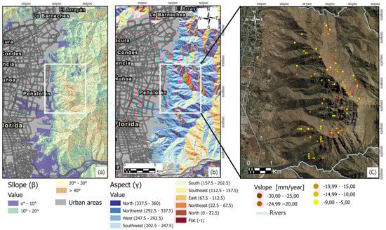
Figure 9.
(a) Slope map with the highest values in pink color, (b) Aspect map indicating the values of the direction of the slopes, with ALOS DEM 30 mts used as background, and (c) Velocities along steepest slope (Vslope map), with Maxar image (source Esri) used as background.
5. Conclusions
The metropolitan area of Santiago de Chile is exposed to numerous natural and anthropic processes that induce regional and local deformations that affect the stability of the basin and its surrounding foothills. GNSS-derived velocities show that the Santiago Basin is tectonically stable, showing typical patterns of interseismic deformation, such as slow eastward motion and uplift. DInSAR allowed us to quantify with excellent spatial resolution areas with local subsidence within the Santiago Basin and landslides in mountainous regions. This allowed us to map the Santiago Basin’s ground stability and investigate the mechanisms responsible for these surface-level variations. Therefore, our study highlights the use of the SAR interferometry technique for the detection of subsidence caused by groundwater exploitation and geohazards related to landslides. Our estimates of surface level changes in the Santiago basin will also be of great importance for urban planning; these results emphasize the mechanical effect of sediment thickness on surface stability and demonstrate how groundwater extraction induces significant land subsidence.
In general, DInSAR shows that the ground surface level in the Santiago basin is relatively stable, but there are areas showing anomalous subsidence. These areas are located in places where groundwater is exploited at the expense of non-renewable storage in aquifer systems, which causes land subsidence and other environmental impacts such as the degradation of water quality, spring discharge, and flow reduction from the rivers. In Quilicura, north of Santiago, the exploitation and compaction of the aquifer is more evident, and a criticality is noted. For Paine, the southern area of Santiago, the deformations have been more evident in recent years, which are influenced by intensive agriculture in the area. On the other hand, although the area is located in the Chilean subduction area, there is no evidence of large deformations influenced by tectonic movement, in particular, movement linked to the San Ramon fault activity. However, we do not rule out that the fault is active and that more observation time is needed to estimate potential deformations across the fault.
Our results show a constant evolution in the subsidence of the anomalous zones, indicating that water withdrawals have continued to affect soil stability during the observed period. This work also provides semi-theoretical relationships in Section 4.3.1 to link information on metropolitan-scale groundwater use with compaction and storage loss, which could allow predictions of subsidence rates and volumes for different groundwater management scenarios.
In the reliefs of the Andes mountain range, using SAR interferometry, we were able to record information in places with difficult access, quickly and efficiently, and detect numerous control points obtained with the SAR sensor. Based on the Vslope projection, we were able to estimate the velocities and determine the status of the movement of the slopes, comparing them with the susceptibility catalogs of landslides to obtain reliable results. Our results highlight the potential of interferometry to identify landslides; however, more information, such as materials, type of geomorphological units, and meteorological data, is required in situ in order to confirm and define more precisely the activity of the phenomenon and the types of movements present in the area. Our study demonstrates that InSAR provides a spatial accuracy that allows for the detection of ground instabilities in areas above ~500 m2. The interferograms have an excellent consistency in the analyzed urban areas of the Santiago basin. In mountainous regions there may be topographic effects that incorporate noise into ground motion estimates, which is why we limited ourselves to using only the descending orbit for landslide identification. Furthermore, the integration of geological information enabled us to interpret the observed ground elevation anomalies in the Santiago Basin. Our results highlight that the thickness of the basin is a key factor for ground stability; in contrast, groundwater extraction induces local instability. These results are fundamental for urban territorial planning in the city of Santiago and demonstrate the importance of geodetic measurements in assessing the impact of climate change on groundwater storage and how this affects the ground surface elevation.
Author Contributions
Conceptualization, F.O., M.M. and G.Y.; methodology, F.O., M.M. and G.Y.; SAR data processing, F.O., validation G.Y. and M.M.; writing F.O., M.M. and G.Y.; supervision, M.M. and G.Y. All authors have read and agreed to the published version of the manuscript.
Funding
This study was supported by the Millennium Nucleus CYCLO (The Seismic Cycle Along Subduction Zones) (ICM) grant NC160025.
Data Availability Statement
The geological maps in Yanez et al. [3]. The catalog of active faults is available at: https://fallasactivas.cl/ (accessed on 10 September 2022, under license https://creativecommons.org/licenses/by/4.0/. The Hydrogeological Data are available on the portal of the DGA 2000, Chilean public water directorate https://dga.mop.gob.cl/servicioshidrometeorologicos/Paginas/default.aspx (accessed on 15 September 2022). Landslide catalogs are available in the master thesis under license https://creativecommons.org/licenses/by-nc-nd/3.0/cl/ (accessed on 10 October 2022).
Acknowledgments
F.O. acknowledges support from the ESA NoR Project ID: 65514. M.M. acknowledges support from the ANID PIA Anillo ACT192169, and National Research Center for Integrated Natural Disaster Management (CIGIDEN).
Conflicts of Interest
The authors declare no conflict of interest.
References
- National Institute of Statistics of Chile, Census Report 2017. Available online: https://www.ine.cl/censo (accessed on 31 October 2022).
- Pastén, C.; Sáez, M.; Ruiz, S.; Leyton, F.; Salomón, J.; Poli, P. Deep characterization of the Santiago Basin using HVSR and cross-correlation of ambient seismic noise. Eng. Geol. 2016, 201, 57–66. [Google Scholar] [CrossRef]
- Yáñez, G.; Muñoz, M.; Flores Aqueveque, V.; Bosch, A. Gravity derived depth to basement in Santiago Basin, Chile: Implications for its geological evolution, hydrogeology, low enthalpy geothermal, soil characterization and geo-hazards. Andean Geol. 2015, 42, 147–172. [Google Scholar] [CrossRef]
- González, F.A.; Maksymowicz, A.; Díaz, D.; Villegas, L.; Leiva, M.; Blanco, B.; Bonvalot, S. Characterization of the depocenters and the basement structure, below the central Chile Andean Forearc: A 3D geophysical modelling in Santiago Basin area. Basin Res. 2018, 30, 799–815. [Google Scholar] [CrossRef]
- Leyton, F.; Sepúlveda, S.A.; Astroza, M.; Rebolledo, S.; Acevedo, P.; Ruiz, S.; Foncea, C. Seismic zonation of the Santiago basin, Chile. In Proceedings of the 5th International Conference on Earthquake Geotechnical Engineering, Santiago, Chile, 10–13 January 2011. [Google Scholar]
- Leyton, F.; Pérez, A.; Campos, J.; Rauld, R.; Kausel, E. Anomalous seismicity in the lower crust of the Santiago Basin, Chile. Phys. Earth Planet. Inter. 2009, 175, 17–25. [Google Scholar] [CrossRef]
- Armijo, R.; Rauld, R.; Thiele, R.; Vargas, G.; Campos, J.; Lacassin, R.; Kausel, E. The West Andean thrust, the San Ramon fault, and the seismic hazard for Santiago, Chile. Tectonics 2010, 29. [Google Scholar] [CrossRef]
- Vargas, G.; Klinger, Y.; Rockwell, T.K.; Forman, S.L.; Rebolledo, S.; Baize, S.; Armijo, R. Probing large intraplate earthquakes at the west flank of the Andes. Geology 2014, 42, 1083–1086. [Google Scholar] [CrossRef]
- Estay, N.P.; Yanez, G.A.; Maringue, J.I. TEM prospection on quaternary faults: The case of San Ramón Fault (SRF), Central Chile. In AGU Fall Meeting Abstracts; American Geophysical Union: Washington, DC, USA, 2016; Volume 2016, p. NH11A-1716. [Google Scholar]
- Yáñez, G.; Perez-Estay, N.; Araya-Vargas, J.; Sanhueza, J.; Figueroa, R.; Maringue, J.; Rojas, T. Shallow anatomy of the San Ramón Fault (Chile) constrained by geophysical methods: Implications for its role in the Andean deformation. Tectonics 2020, 39, e2020TC006294. [Google Scholar] [CrossRef]
- van Dinther, Y.; Preiswerk, L.E.; Gerya, T.V. A secondary zone of uplift due to megathrust earthquakes. Pure Appl. Geophys. 2019, 176, 4043–4068. [Google Scholar] [CrossRef]
- Mosca, I.; Console, R.; d’Addezio, G. Renewal models of seismic recurrence applied to paleoseismological and historical observations. Tectonophysics 2012, 564, 54–67. [Google Scholar] [CrossRef]
- Santibáñez, I.; Cembrano, J.; García-Pérez, T.; Costa, C.; Yáñez, G.; Marquardt, C.; González, G. Crustal faults in the Chilean Andes: Geological constraints and seismic potential. Andean Geol. 2018, 46, 32–65. [Google Scholar] [CrossRef]
- Peltier, W.R. Global glacial isostasy and the surface of the ice-age Earth: The ICE-5G (VM2)model and GRACE. Annu. Rev. Earth Planet. Sci. 2004, 32, 111–149. [Google Scholar] [CrossRef]
- Kooi, H.; de Vries, J. Land subsidence and hydrodynamic compaction of sedimentarybasins. Hydrol. Earth Syst. Sci. 1998, 2, 159–171. [Google Scholar] [CrossRef]
- White, A.M.; Gardner, W.P.; Borsa, A.A.; Argus, D.F.; Martens, H.R. A review of GNSS/GPS in hydrogeodesy: Hydrologic loading applications and their implications for water resource research. Water Resour. Res. 2022, 58, e2022WR032078. [Google Scholar] [CrossRef] [PubMed]
- Minderhoud, P.; Middelkoop, H.; Erkens, G.; Stouthamer, E. Groundwater extraction may drown mega-delta: Projections of extraction-induced subsidence and elevation of the Mekong delta for the 21st century. Environ. Res. Commun. 2019, 2, 011005. [Google Scholar] [CrossRef]
- Chen, B.; Gong, H.; Chen, Y.; Li, X.; Zhou, C.; Lei, K.; Zhu, L.; Duan, L.; Zhao, X. Land subsidence and its relation with groundwater aquifers in Beijing Plain of China. Sci. Total Environ. 2020, 735, 139111. [Google Scholar] [CrossRef]
- Turner, R.E.; Mo, Y. Salt Marsh Elevation limit determined after subsidence from hydrologic change and hydro-carbon extraction. Remote Sens. 2021, 13, 49. [Google Scholar] [CrossRef]
- Singh, A.; Rao, G.S. Crustal structure and subsidence history of the Mannar basin through potential field modelling and backstripping analysis: Implications on basin evolution and hydrocarbon exploration. J. Pet. Sci. Eng. 2021, 206, 109000. [Google Scholar] [CrossRef]
- Gahramanov, G.; Babayev, M.; Shpyrko, S.; Mukhtarova, K. Subsidence history and hydrocarbon migration modeling in south caspian basin. Visnyk Taras Shevchenko Natl. Univ. Kyiv. Geol. 2020, 1, 82–91. [Google Scholar] [CrossRef]
- Stramondo, S.; Bozzano, F.; Marra, F.; Wegmuller, U.; Cinti, F.; Moro, M.; Saroli, M. Subsidence induced by urbanisation in the city of Rome detected by advanced InSAR technique and geotechnical investigations. Remote Sens. Environ. 2008, 112, 3160–3172. [Google Scholar] [CrossRef]
- Manunta, M.; Marsella, M.; Zeni, G.; Sciotti, M.; Atzori, S.; Lanari, R. Two-scale surface deformation analysis using the SBAS-DInSAR technique: A case study of the city of Rome, Italy. Int. J. Remote Sens. 2008, 29, 1665–1684. [Google Scholar] [CrossRef]
- Abidin, H.Z.; Andreas, H.; Djaja, R.; Darmawan, D.; Gamal, M. Land subsidence characteristics of Jakarta between 1997 and 2005, as estimated using GPS surveys. GPS Solut. 2008, 12, 23–32. [Google Scholar] [CrossRef]
- Orellana, F.; Blasco, J.D.; Foumelis, M.; D’Aranno, P.; Marsella, M.; Di Mascio, P. DInSAR for Road Infrastructure Monitoring: Case Study Highway Network of Rome Metropolitan (Italy). Remote Sens. 2020, 12, 3697. [Google Scholar] [CrossRef]
- Chang, L.; Dollevoet, R.P.B.J.; Hanssen, R.F. Monitoring Line-Infrastructure with Multisensor SAR Interferometry: Products and Performance Assessment Metrics. IEEE J. Sel. Top. Appl. Earth Obs. Remote Sens. 2018, 11, 1593–1605. [Google Scholar] [CrossRef]
- Li, S.; Xu, W.; Li, Z. Review of the SBAS InSAR Time-series algorithms, applications, and challenges. Geod. Geodyn. 2021, 13, 114–126. [Google Scholar] [CrossRef]
- Orellana, F.; Hormazábal, J.; Montalva, G.; Moreno, M. Measuring Coastal Subsidence after Recent Earthquakes in Chile Central Using SAR Interferometry and GNSS Data. Remote Sens. 2022, 14, 1611. [Google Scholar] [CrossRef]
- Delouis, B.; Nocquet, J.M.; Vallée, M. Slip distribution of the February 27, 2010 Mw = 8.8 Maule earthquake, central Chile, from static and high-rate GPS, InSAR, and broadband teleseismic data. Geophys. Res. Lett. 2010, 37, 17. [Google Scholar] [CrossRef]
- van Natijne, A.L.; Bogaard, T.A.; van Leijen, F.J.; Hanssen, R.F.; Lindenbergh, R.C. World-wide insar sensitivity index for landslide deformation tracking. Int. J. Appl. Earth Obs. Geoinf. 2022, 111, 102829. [Google Scholar] [CrossRef]
- Fobert, M.A.; Singhroy, V.; Spray, J.G. InSAR monitoring of landslide activity in Dominica. Remote Sens. 2021, 13, 815. [Google Scholar] [CrossRef]
- Moretto, S.; Bozzano, F.; Mazzanti, P. The role of satellite InSAR for landslide forecasting: Limitations and openings. Remote Sens. 2021, 13, 3735. [Google Scholar] [CrossRef]
- De Corso, T.; Mignone, L.; Sebastianelli, A.; del Rosso, M.P.; Yost, C.; Ciampa, E.; Ullo, S. Application of DInSAR technique to high coherence satellite images for strategic infrastructure monitoring. In IGARSS 2020-2020 IEEE International Geoscience and Remote Sensing Symposium; IEEE: Piscataway, NJ, USA, 2020; pp. 4235–4238. [Google Scholar] [CrossRef]
- D’Aranno, P.; Di Benedetto, A.; Fiani, M.; Marsella, M. Remote sensing technologies for linear infrastructure monitoring. Int. Arch. Photogramm. Remote Sens. Spat. Inf. Sci. 2019, 42, 461–468. [Google Scholar] [CrossRef]
- Bonì, R.; Herrera, G.; Meisina, C.; Notti, D.; Béjar-Pizarro, M.; Zucca, F.; González, P.J.; Palano, M.; Tomás, R.; Fernández, J.; et al. Twenty-year advanced DInSAR analysis of severe land subsidence: The Alto Guadalentín Basin (Spain) case study. Eng. Geol. 2015, 198, 40–52. [Google Scholar] [CrossRef]
- Ezquerro, P.; Tomás, R.; Béjar-Pizarro, M.; Fernández-Merodo, J.A.; Guardiola-Albert, C.; Staller, A.; Sánchez-Sobrino, J.A.; Herrera, G. Improving multi—Technique monitoring using Sentinel-1 and Cosmo-SkyMed data and upgrading groundwater model capabilities. Sci. Total Environ. 2019, 703, 134757. [Google Scholar] [CrossRef] [PubMed]
- Taftazani, R.; Kazama, S.; Takizawa, S. Spatial Analysis of Groundwater Abstraction and Land Subsidence for Planning the Piped Water Supply in Jakarta, Indonesia. Water 2022, 14, 3197. [Google Scholar] [CrossRef]
- Ferretti, A.; Prati, C.; Rocca, F. Permanent scatterers in SAR interferometry. IEEE Trans. Geosci. Remote Sens. 2001, 39, 8–20. [Google Scholar] [CrossRef]
- Berardino, P.; Fornaro, G.; Lanari, R.; Sansosti, E. A new algorithm for surface deformation monitoring based on small baseline differential SAR interferograms. IEEE Trans. Geosci. Remote Sens. 2002, 40, 2375–2383. [Google Scholar] [CrossRef]
- Crosetto, M.; Monserrat, O.; Cuevas-González, M.; Devanthéry, N.; Crippa, B. Persistent Scatterer Interferometry: A Review. ISPRS J. Photogramm. Remote Sens. 2016, 115, 78–89. [Google Scholar] [CrossRef]
- Ferretti, A.; Fumagalli, A.; Novali, F.; Prati, C.; Rocca, F.; Rucci, A. A New Algorithm for Processing Interferometric Data-Stacks: SqueeSAR. IEEE Trans. Geosci. Remote Sens. 2011, 49, 3460–3470. [Google Scholar] [CrossRef]
- Hooper, A.J. A Multi-Temporal InSAR Method Incorporating Both Persistent Scatterer and Small Baseline Approaches. Geophys. Res. Lett. 2008, 35. [Google Scholar] [CrossRef]
- Casu, F.; Elefante, E.; Imperatore, P.; Zinno, I.; Manunta, M.; De Luca, C.; Lanari, R. SBAS-DInSAR Parallel Processing for Deformation Time Series Computation. IEEE JSTARS 2004, 7, 3285–3296. [Google Scholar] [CrossRef]
- European Space Agency. Sentinel-1—Missions—Sentinel. Available online: https://sentinel.esa.int/web/sentinel/missions/sentinel-1 (accessed on 13 July 2022).
- Manunta, M.; De Luca, C.; Zinno, I.; Casu, F.; Manzo, M.; Bonano, M.; Fusco, A.; Pepe, A.; Onorato, G.; Berardino, P.; et al. The Parallel SBAS Approach for Sentinel-1 Interferometric Wide Swath Deformation Time-Series Generation: Algorithm Description and Products Quality Assessment. IEEE Trans. Geosci. Remote Sens. 2019, 57, 6259–6281. [Google Scholar] [CrossRef]
- De Luca, C.; Cuccu, R.; Elefante, S.; Zinno, I.; Manunta, M.; Casola, V.; Rivolta, G.; Lanari, R.; Casu, F. An On-Demand Web Tool for the Unsupervised Retrieval of Earth’s Surface Deformation from SAR Data: The P-SBAS Service within the ESA G-POD Environment. Remote Sens. 2015, 7, 15630–15650. [Google Scholar] [CrossRef]
- Manunta, M.; Casu, F.; Zinno, I.; de Luca, C.; Pacini, F.; Brito, F.; Blanco, P.; Iglesias, R.; Lopez, A.; Briole, P.; et al. The Geohazards Exploitation Platform: An advanced cloud-based environment for the Earth Science community. In Proceedings of the 19th EGU General Assembly, EGU2017, Vienna, Austria, 23–28 April 2017; p. 14911. [Google Scholar]
- Foumelis, M.; Papadopoulou, T.; Bally, P.; Pacini, F.; Provost, F.; Patruno, J. Monitoring Geohazards Using On-Demand and Systematic Services on Esa’s Geohazards Exploitation Platform. In Proceedings of the IGARSS 2019, IEEE International Geoscience and Remote Sensing Symposium, Yokohama, Japan, 28 July–2 August 2019; IEEE: Piscataway, NJ, USA, 2019; pp. 5457–5460. [Google Scholar] [CrossRef]
- Galve, J.P.; Pérez-Peña, J.V.; Azañón, J.M.; Closson, D.; Calò, F.; Reyes-Carmona, C.; Jabaloy, A.; Ruano, P.; Mateos, R.M.; Notti, D.; et al. Evaluation of the SBAS InSAR Service of the European Space Agency’s Geohazard Exploitation Platform (GEP). Remote Sens. 2017, 9, 1291. [Google Scholar] [CrossRef]
- Reyes-Carmona, C.; Galve, J.P.; Barra, A.; Monserrat, O.; María Mateos, R.; Azañón, J.M.; Perez-Pena, J.V.; Ruano, P. The Sentinel-1 CNR-IREA SBAS service of the European Space Agency’s Geohazard Exploitation Platform (GEP) as a powerful tool for landslide activity detection and monitoring. In Proceedings of the EGU General Assembly, Vienna, Austria, 3–8 May 2020; p. 19410. [Google Scholar]
- Moreno, M.; Rosenau, M.; Oncken, O. Maule earthquake slip correlates with pre-seismic locking of Andean subduction zone. Nature 2010, 467, 198–202. [Google Scholar] [CrossRef] [PubMed]
- Tilmann, F.; Zhang, Y.; Moreno, M.; Saul, J.; Eckelmann, F.; Palo, M.; Deng, Z.; Babeyko, A.; Chen, K.; Báez, J.C.; et al. The 2015 Illapel earthquake, central Chile: A type case for a characteristic earthquake? Geophys. Res. Lett. 2016, 43, 574–583. [Google Scholar] [CrossRef]
- Carvajal, M.; Cisternas, M.; Catalán, P.A. Source of the 1730 Chilean earthquake from historical records: Implications for the future tsunami hazard on the coast of Metropolitan Chile. J. Geophys. Res. Solid Earth 2017, 122, 3648–3660. [Google Scholar] [CrossRef]
- Sippl, C.; Moreno, M.; Benavente, R. Microseismicity appears to outline highly coupled regions on the Central Chile megathrust. J. Geophys. Res. Solid Earth 2021, 126, e2021JB022252. [Google Scholar] [CrossRef]
- Maldonado, V.; Contreras, M.; Melnick, D. A comprehensive database of active and potentially-active continental faults in Chile at 1:25,000 scale. Sci. Data 2021, 8, 20. [Google Scholar] [CrossRef]
- Donoso, F.; Moreno, M.; Ortega-Culaciati, F.; Bedford, J.; Benavente, R. Automatic Detection of Slow Slip Events Using the PICCA: Application to Chilean GNSS Data. Front. Earth Sci. 2021, 9, 788054. [Google Scholar] [CrossRef]
- Charrier, R.; Farías, M.; Maksaev, V. Evolución tectónica, paleogeográfica y metalogénica durante el Cenozoico en los Andes de Chile norte y central e implicaciones para las regiones adyacentes de Bolivia y Argentina. Rev. Asoc. Geológica Argent. 2009, 65, 5–35. [Google Scholar]
- Pardo-Casas, F.; Molnar, P. Relative motion of the Nazca (Farallon) and South American plates since Late Cretaceous time. Tectonics 1987, 6, 233–248. [Google Scholar] [CrossRef]
- Godoy, E.; Lara, L. Segmentación estructural andina a los 33-34: Nuevos datos en la Cordillera Principal. In Congreso Geológico Chileno; Universidad de Concepción, Departamento Ciencias de la Tierra: Concepción, Chile, 1994; pp. 1344–1348. [Google Scholar]
- Wyss, A.R.; Flynn, J.J.; Norell, M.; Swisher, C.C.; Novacek, M.J.; McKenna, M.C.; Charrier, R. Paleogene mammals from the Andes of central Chile: A preliminary taxonomic, biostratigraphic, and geochronologic assessment. Am. Mus. Novit. 1994, 5, 3098. [Google Scholar]
- Charrier, R.; Baeza, O.; Elgueta, S.; Flynn, J.J.; Gans, P.; Kay, S.M.; Zurita, E. Evidence for Cenozoic extensional basin development and tectonic inversion south of the flat-slab segment, southern Central Andes, Chile (33–36 SL). J. South Am. Earth Sci. 2002, 15, 117–139. [Google Scholar] [CrossRef]
- Charrier, R.; Bustamante, M.; Comte, D.; Elgueta, S.; Flynn, J.J.; Iturra, N.; Wyss, A.R. The Abanico extensional basin: Regional extension, chronology of tectonic inversion and relation to shallow seismic activity and Andean uplift. Neues Jahrb. Für Geol. Und Paläontologie Abh. 2005, 236, 43–77. [Google Scholar] [CrossRef]
- Fock, A.; Charrier, R.; Farías, M.; Muñoz, M. Fallas de vergencia oeste en la Cordillera Principal de Chile Central: Inversión de la cuenca de Abanico (33-34 S). Rev. Asoc. Geológica Argent. Publicación Espec. 2006, 6, 48–55. [Google Scholar]
- Moreno, T.; Gibbons, W.; Cembrano, J.; Lavenue, A.; Yáñez, G. (Eds.) The Geology of Chile, Chapter 9; Geological Society of London: London, UK, 2007. [Google Scholar]
- Farías, M.; Vargas, G.; Tassara, A.; Carretier, S.; Baize, S.; Melnick, D.; Bataille, K. Land-level changes produced by the M w 8.8 2010 Chilean earthquake. Science 2010, 329, 916. [Google Scholar] [CrossRef] [PubMed]
- Garreaud, R.D.; Alvarez-Garreton, C.; Barichivich, J.; Boisier, J.P.; Christie, D.; Galleguillos, M.; LeQuesne, C.; McPhee, J.; Zambrano-Bigiarini, M. The 2010–2015 megadrought in central Chile: Impacts on regional hydroclimate and vegetation. Hydrol. Earth Syst. Sci. 2017, 21, 6307–6327. [Google Scholar] [CrossRef]
- Torres, R.; Snoeij, P.; Geudtner, D.; Bibby, D.; Davidson, M.; Attema, E.; Rostan, F. GMES Sentinel-1 mission. Remote Sens. Environ. 2012, 120, 9–24. [Google Scholar] [CrossRef]
- Cigna, F.; Tapete, D. Sentinel-1 big data processing with P-SBAS InSAR in the geohazards exploitation platform: An experiment on coastal land subsidence and landslides in Italy. Remote Sens. 2021, 13, 885. [Google Scholar] [CrossRef]
- Farr, T.G.; Rosen, P.A.; Caro, E.; Crippen, R.; Duren, R.; Hensley, S.; Kobrick, M.; Paller, M.; Rodriguez, E.; Roth, L.; et al. The Shuttle Radar Topography Mission. Rev. Geophys. 2007, 45, RG2004. [Google Scholar] [CrossRef]
- Yague-Martinez, N.; De Zan, F.; Prats-Iraola, P. Coregistration of Interferometric Stacks of Sentinel-1 TOPS Data. IEEE Geosci. Remote Sens. Lett. 2017, 14, 1002–1006. [Google Scholar] [CrossRef]
- Cascini, L.; Fornaro, G.; Peduto, D. Advanced low- and full-resolution DInSAR map generation for slow-moving landslide analysis at different scales. Eng. Geol. 2010, 112, 29–42. [Google Scholar] [CrossRef]
- Cigna, F.; Bianchini, S.; Casagli, N. How to assess landslide activity and intensity with Persistent Scatterer Interferometry (PSI): The PSI-based matrix approach. Landslides 2013, 10, 267–283. [Google Scholar] [CrossRef]
- Barría, P.; Chadwick, C.; Ocampo-Melgar, A.; Galleguillos, M.; Garreaud, R.; Díaz-Vasconcellos, R.; Poblete-Caballero, D. Water management or megadrought: What caused the Chilean Aculeo Lake drying? Reg. Environ. Chang. 2021, 21, 19. [Google Scholar] [CrossRef]
- Ocampo-Melgar, A.; Barria, P.; Chadwick, C.; Villoch, P. Restoration perceptions and collaboration challenges under severe water scarcity: The Aculeo Lake process. Restor. Ecol. 2021, 29, e13337. [Google Scholar] [CrossRef]
- DGA. Modelo de Simulación Hidrológico Operacional: Cuencas de los ríos Maipo y Mapocho; Ayala, Cabrera y Asociados; Series SIT; Dirección General de Aguas, Ministerio de Obras Públicas: Santiago, Chile, 2000; p. 87.
- Terzaghi, K. Principles of soil mechanics: IV. Settlement and consolidation of clay. Erdbaummechanic 1925, 95, 874–878. [Google Scholar]
- Biot, M. General theory of three-dimensional consolidation. J. Appl. Phys. 1941, 12, 155–164. [Google Scholar] [CrossRef]
- Castellazzi, P.; Martel, R.; Rivera, A.; Huang, J.; Pavlic, G.; Calderhead, A.I.; Chaussard, E.; Garfias, J.; Salas, J. Groundwater depletion in Central Mexico: Use of GRACE and InSAR to support water resources management. Water Resour. Res. 2016, 52, 5985–6003. [Google Scholar] [CrossRef]
- Mourad, M.; Tsuji, T.; Ikeda, T.; Ishitsuka, K.; Senna, S.; Ide, K. Mapping Aquifer Storage Properties Using S-Wave Velocity and InSAR-Derived Surface Displacement in the Kumamoto Area, Southwest Japan. Remote Sens. 2021, 13, 4391. [Google Scholar] [CrossRef]
- Miller, M.M.; Shirzaei, M.; Argus, D. Aquifer mechanical properties and decelerated compaction in Tucson, Arizona. J. Geophys. Res. Solid Earth 2017, 122, 8402–8416. [Google Scholar] [CrossRef]
- Antinao, J.; Fernández, J.C.; Naranjo, J.A.; Villarroel, P. Peligro de Remociones en Masa e Inundaciones de la Cuenca de Santiago, Región Metropolitana. Servicio Nacional de Geología y Minería, Carta Geológica de Chile, Serie Geología Ambiental 2, 1 Mapa Escala 1:100,000. Santiago 2003. Available online: https://snia.mop.gob.cl/repositoriodga/handle/20.500.13000/3929 (accessed on 15 September 2022).
- Sepúlveda, S.A.; Padilla, C. Rain-induced debris and mudflow triggering factors assessment in the Santiago cordilleran foothills, Central Chile. Nat. Hazards 2008, 47, 201–215. [Google Scholar] [CrossRef]
- Naranjo, J.A.; Varela, J. Flows of debris and mud that affected the eastern sector of Santiago on May 3, 1993. Natl. Serv. Geol. Min. Bull. 1996, 47, 42. [Google Scholar]
- Lara, M.; Sepúlveda, S.A.; Celis, C.; Rebolledo, S.; Ceballos, P. Landslide susceptibility maps of Santiago city Andean foothills, Chile. Andean Geol. 2018, 45, 433–442. [Google Scholar] [CrossRef]
- Sepúlveda, S.A.; Moreiras, S.M.; Lara, M.; Alfaro, A. Debris flows in the Andean ranges of central Chile and Argentina triggered by 2013 summer storms: Characteristics and consequences. Landslides 2015, 12, 115–133. [Google Scholar] [CrossRef]
- Celis Saez, C. Susceptibility of Mass Removals and Danger of Flows in the Andean Front of Santiago, Metropolitan Region. 2018. Available online: https://repositorio.uchile.cl/handle/2250/168618 (accessed on 10 October 2022).
- Colesanti, C.; Wasowski, J. Investigating landslides with space-borne Synthetic Aperture Radar (SAR) interferometry. Eng. Geol. 2006, 88, 173–199. [Google Scholar] [CrossRef]
- Plank, S.; Singer, J.; Minet, C.; Thuro, K. Pre-survey suitability evaluation of the differential synthetic aperture radar interferometry method for landslide monitoring. Int. J. Remote Sens. 2012, 33, 6623–6637. [Google Scholar] [CrossRef]
Publisher’s Note: MDPI stays neutral with regard to jurisdictional claims in published maps and institutional affiliations. |
© 2022 by the authors. Licensee MDPI, Basel, Switzerland. This article is an open access article distributed under the terms and conditions of the Creative Commons Attribution (CC BY) license (https://creativecommons.org/licenses/by/4.0/).