Article

Autoencoder Neural Network-Based STAP Algorithm for Airborne Radar with Inadequate Training Samples

1
National Laboratory of Radar Signal Processing, Xidian University, Xi’an 710071, China
2
Computer Science Program, University of Southampton Malaysia, Nusajaya 79100, Malaysia
*
Author to whom correspondence should be addressed.
Remote Sens. 2022, 14(23), 6021; https://doi.org/10.3390/rs14236021
Submission received: 14 October 2022 / Revised: 18 November 2022 / Accepted: 23 November 2022 / Published: 28 November 2022
(This article belongs to the Special Issue Small or Moving Target Detection with Advanced Radar System)

Abstract

:
Clutter suppression is a key problem for airborne radar, and space-time adaptive processing (STAP) is a core technology for clutter suppression and moving target detection. However, in practical applications, the non-uniform time-varying environments including clutter range dependence for non-side-looking radar lead to the training samples being unable to satisfy the sample requirements of STAP that they should be independent identical distributed (IID) and that their number should be greater than twice the system’s degree of freedom (DOF). The lack of sufficient IID training samples causes difficulty in the convergence of STAP and further results in a serious degeneration of performance. To overcome this problem, this paper proposes a novel autoencoder neural network for clutter suppression with a unique matrix designed to be decoded and encoded. The main challenges are improving the accuracy of the estimation of the clutter-plus-noise covariance matrix (CNCM) for STAP convergence, designing the form of the data input to the network, and making the network successfully explored to the improvement of CNCM. For these challenges, the main proposed solutions include designing a unique matrix with a certain dimension and a series of covariance data selections and matrix transformations. Consequently, the proposed method compresses and retains the characteristics of the covariances, and abandons the deviations caused by the non-uniformity and the deficiency of training samples. Specifically, the proposed method firstly develops a unique matrix whose dimension is less than half of the DOF, meanwhile, it is based on a processing of the selected clutter-plus-noise covariances. Then, an autoencoder neural network with l 2 regularization and the sparsity regularization is proposed for the unique matrix to be decoded and encoded. The training of the proposed autoencoder can be achieved by reducing the total loss function with the gradient descent iterations. Finally, an inverted processing for the autoencoder output is designed for the reconstruct ion of the clutter-plus-noise covariances. Simulation results are used to verify the effectiveness and advantages of the proposed method. It performs obviously superior clutter suppression for both side-looking and non-side-looking radars with strong clutter, and can deal with the insufficient and the non-uniform training samples. For these conditions, the proposed method provides the relatively narrowest and deepest IF notch. Furthermore, on average it improves the improvement factor (IF) by 10 dB more than the ADC, DW, JDL, and original STAP methods.

1. Introduction

Airborne radar has huge advantages over ground-based radar in far sight and flexibility. When looking down, radar on a moving platform suffers from the core problem of clutter suppression because the ground clutter is strong and its Doppler spectrum is seriously widened due to the platform movement, which further causes the Doppler spectrum of the target to be drowned in the clutter spectrum [1,2,3,4]. For this, the space-time adaptive processing (STAP) of airborne radar has become the core technology for clutter suppression and target detection. With the space-time two-dimensional spectral domain, it obtains a better performance than the traditional one-dimensional processing [4,5,6].
However, estimating the clutter-plus-noise covariance matrix (CNCM) accurately is essential for STAP, which requires that the number of the independent and identically distributed (IID) samples should be greater than twice the system’s degrees of freedom (DOF) to achieve an output signal-to-clutter-plus-noise ratio (SCNR) loss within 3 dB [7]. Unfortunately, due to the array configurations and the complex clutter environment, sufficient training samples are difficult to obtain in non-uniform time-varying environments [8,9]. In particular, as a phenomenon of clutter non-uniformities, the clutter range dependence occurs when the configuration of the array antenna is non-side-looking, which directly results in the training samples failing to meet the IID condition [10]. Therefore, in applications, the difficulty in obtaining enough IID training samples makes the performance of STAP degrade significantly.
Reducing the dimension or rank is often used to solve the problems mentioned above, by decreasing the system’s DOF and selecting parts of the training sample data to estimate the CNCM of the cell to be detected [11,12,13,14]. For example, in STAP dimension reduction methods with fixed structure, the auxiliary channel processing (ACP) method [15] has been proposed by means of setting the two-dimensional beam near the clutter ridge as the auxiliary beam. It reduces the DOF from MN to M+N-1. Utilizing the two-dimensional Fourier transform and simultaneously dealing with beamforming and Doppler frequency processing, a joint domain localized (JDL) [16] method that selects a rectangle joint processing local area is proposed. It reduces the dimension of adaptive processing to the product of length and width of the selected processing local area. Besides, for limited IID training samples, STAP based on the sparse representation (SR) theory called SR-STAP are proposed [17,18,19]. In addition, sparse Bayesian learning (SBL) [20]-based STAP has also received attention because of its robustness. However, their performance relies on the match between the sparse representation of the clutter and the setting of the dictionary matrix; meanwhile, at present most of STAP methods for clutter suppression are based on the side-looking array whose samples are theoretically IID.
Although the above-mentioned methods reduce the consequences of the insufficiency and non-uniformity of the training samples, STAP with low degrees of freedom or reduced samples leads to performance degradation.
For the clutter non-uniformity caused by the clutter range dependence, it can also be solved by range distance compensation and scale transition [21,22,23,24]. Clutter range compensation mainly compensates the clutter spectra of adjacent training cells so that the space-time distribution characteristics of the clutter after compensation are as consistent as possible to those to be detected. Thus, the performance of the clutter suppression of the follow-up STAP processing can be improved. For example, Borsari proposed the Doppler warping (DW) algorithm [25,26] based on the non-side-looking array. The Doppler frequencies of the range cells to be detected and compensated are obtained by using the inertial navigation parameters of the radar system. The two-dimensional clutter spectra of the range cells to be compensated for are shifted into one dimension so that in the Doppler frequency direction, they coincide with the clutter spectrum of the range cell to be detected. Then, the correlation of the range distance of the clutter is eliminated. Furthermore, Klemm proposes an angle-Doppler compensation (ADC) method [27] which obtains the Doppler frequency of each range cell through adaptive estimation of the echo data, rather than through the inertial navigation parameters of the system. Additionally, Pearson proposed the high-order Doppler warping (HODW) method [28], which compensates the adjacent range cells from multiple spatial angle directions. However, the existing methods are hardly able to take both the insufficiency of training samples and the non-uniformity, such as the clutter range dependence caused by the non-side-looking array, into consideration at the same time.
In this paper, we propose an autoencoder neural network-based STAP algorithm for airborne radar with inadequate training samples. The aim of this paper is to overcome the lack of sufficient IID training samples, and even to overcome the non-uniform samples that cannon obey the IID condition. The novel method firstly based on a processing of the selected clutter-plus-noise covariances designs a unique matrix whose dimension is less than half of the DOF. Next, an autoencoder neural network with l 2 regularization and sparsity regularization is proposed for the unique matrix to be decoded and encoded. Then, the training of neural network of the proposed autoencoder is achieved by reducing the total loss function with the gradient descent iterations. Finally, the invert processing for the output of the autoencoder is designed for the reconstruction of the clutter-plus-noise covariances. Compared to the conventional methods, it performs obviously superior clutter suppression for both side-looking and non-side-looking radars with strong clutter and improves the improvement factor (IF) greatly. The proposed method can adapt better to non-uniform clutter environments and non-ideal sample conditions. In this paper, the non-uniformity of samples mainly refers to those caused by clutter range dependence in non-side-looking arrays.
Notation: ( · ) H , ( · ) 1 and ( · ) * denote conjugate-transpose, inverse, and conjugate operators, respectively. ⊗ and ⊙ denote the Kronecker and the Khatri–Rao product operators, respectively. ( · ) ( · ) denotes the derivative. C K × 1 denotes the K × 1 dimension.

2. Signal Model

Consider an airborne monostatic radar system equipped witha uniform linear array (ULA) whose number of the receiving array elements is N. The elements are half-wavelength d = λ / 2 inner spaced, and K pulses are transmitted at a constant pulse repetition frequency (PRF) f P R F during a coherent processing interval (CPI). A range cell is composed of all the clutter scattering cells which hold the same slant distance as the antenna array, and the components from different scatterers in the clutter echo are independent of each other. For the antenna array and the clutter scatterers, it is assumed that the platform is moving at a uniform speed v a , and the angle (non-side-looking angle) between the ULA and the moving direction of the platform is ϑ . Moreover, the angle between the clutter scatterers and the antenna array is α , and the angle between the clutter scatterers and the moving direction of the platform is β . Furthermore, relative to the speed vector of the platform, the elevation angle and the azimuth angle of the clutter scatterers are θ and φ , respectively. Then, each column of N × K dimensional echo data matrix collected from K pulses in a CPI is stacked to obtain a vector x c n , l , as follows [29,30]
x c n , l = i = 1 N c ξ i , l a s t ( f s , i , f d , i ) + n l
where N c is the total number of the clutter blocks in the clutter cell, and ξ i , l is the complex amplitude of the ith clutter block in the clutter cell. The l stands for the lth range cell. Meanwhile, a s t ( f s , i , f d , i ) is the space-time steering vector of the ith clutter block, and n l is the zero-mean noise vector. In Equation (1), the space-time two-dimensional steering vector a s t ( f s , i , f d , i ) can be expressed in detail as
a s t ( f s , i , f d , i ) = a t ( f d , i ) a s ( f s , i )
in which the temporal steering vector a t ( f d , i ) is expressed as
a t ( f d , i ) = [ 1 , e j 2 π f d , i f P R F , , e j 2 π ( K 1 ) f d , i f P R F ] C K × 1
and the spatial steering vector a s ( f s , i ) is
a s ( f s , i ) = [ 1 , e j 2 π f s , i , , e j 2 π ( N 1 ) f s , i ] C N × 1
where f d , i f P R F and f s , i are the normalized spatial frequency and Doppler frequency, respectively. According to the spatial geometric relationship, the Doppler frequency f d , i of the clutter scatterer can be written as
f d , i = 2 v a λ cos ( θ i ) cos ( φ i ) = 2 v a λ cos ( β i )
where β i is the spatial cone angle. In addition, the spatial frequency of the scatterer is
f s , i = d λ cos ( α i ) = d λ cos ( θ i ) cos ( φ i ϑ i )
The all-space-time adaptive processing means that all the space and the time degrees of freedom are used in the process of clutter suppression. The purpose of STAP is to suppress clutter as much as possible and keep the target gain of the output unchanged. Thus, according to the linear constraint minimum variance (LCMV) criterion, the adaptive optimal weight vector w o p t can be obtained from the following formula
min w w H R X w , s . t . w H a s t ( f s 0 , f d 0 ) = 1
where a s t ( f s 0 , f d 0 ) is the space-time steering vector of the target and f d 0 and f s 0 are its temporal frequency and spatial frequency. According to the Lagrange multiplier method, the optimal weight vector w o p t can be obtained from
w o p t = R X 1 a s t ( f s 0 , f d 0 ) a s t H ( f s 0 , f d 0 ) R X 1 a s t ( f s 0 , f d 0 )
where w o p t is the weight vector of STAP and a s t ( f s 0 , f d 0 ) is the space-time vector with N K × 1 dimension. R X is the covariance matrix, and in practical applications, R X is unknown. Therefore, maximum likelihood estimation is usually used to estimate the covariance matrix, as follows [31]:
R X R ^ X = 1 L l = 1 L x ( l ) x H ( l )
where x ( l ) for l = 1 , 2 , , L are the training samples near the cell to be detected and they exclude samples with a strong clutter scattering point or suspected target pollution. L is the total number of the training samples used to estimate R ^ X . By solving Equation (7) with R ^ X , the optimal space-time weight vector w o p t can be obtained.
It should be mentioned that according to the formula transformation of the sum-difference angle, for the clutter scatterer, the relationship between its spatial frequency and Doppler frequency is
[ f d f d m cos ( α ) cos ( ϑ ) ] 2 + cos 2 ( α ) sin 2 ( ϑ ) = cos 2 ( θ ) sin 2 ( ϑ )
When the antenna is a positive side-looking structure with ϑ = 0 , which means that the array direction is consistent with the moving direction of platform, the clutter spectrum is linearly distributed on the space-time two-dimensional plane and has range stability. When the antenna is a forward-looking structure, that is ϑ = 90 , the trajectory of the clutter spectrum in the space-time two-dimensional plane is a cluster of ellipses, and the radii of the ellipses change with distance. When the antenna is a non-side-looking structure with 0 < ϑ < 90 , the clutter spectrum in the space-time two-dimensional plane presents an oblique elliptical distribution, and the radii of the ellipses change with distance. Therefore, the corresponding training samples do not meet the IID condition.

3. The Proposed Algorithm

For the covariance matrix R ^ X c n ( i , j ) of clutter-plus-noise, its element can by calculated by
R ^ X c n ( i , j ) = X c n ( i , : ) X c n H ( j , : ) = 1 L l = 1 L X c n ( i , l ) X c n * ( j , l ) ( 1 i , j N K )
where T ¯ ( k 1 , k 2 ) generally stands for the element of T ¯ located at the k 1 th row and the k 2 th column, and T ¯ ( k 1 , : ) is the k 1 th row of the matrix T ¯ . X c n is composed of X c n = [ x c n , 1 , , x c n , L ] . The proposed method designs a unique sub-matrix to be decoded and encoded based on the following construction
R ^ X c n = R ^ ( 1 ) c n C p × ( N K p ) R ^ ( 2 ) c n C p × p R ^ ( 3 ) c n C ( N K p ) × ( N K p ) R ^ ( 4 ) c n C ( N K p ) × p , p < N K 2
where the size of the dimension p is designed as p < N K / 2 in the proposed method, which means that p is a positive integer that is not too large and less than half of the system’s degree of freedom. In detail, the expression of R ^ ( 2 ) c n is
R ^ ( 2 ) c n = 1 L l = 1 L X c n ( 1 , l ) X c n * ( N K p + 1 , l ) X c n ( 1 , l ) X c n * ( N K p + 2 , l ) X c n ( 1 , l ) X c n * ( N K , l ) X c n ( 2 , l ) X c n * ( N K p + 1 , l ) X c n ( 2 , l ) X c n * ( N K p + 2 , l ) X c n ( 2 , l ) X c n * ( N K , l ) X c n ( p , l ) X c n * ( N K p + 1 , l ) X c n ( p , l ) X c n * ( N K p + 2 , l ) X c n ( p , l ) X c n * ( N K , l )
where R ^ ( 2 ) c n contains parts of the clutter-plus-noise covariances. Then, for the reconstruction of the CNCM, a unique matrix is proposed as follows:
C r e = [ R ^ ( 2 ) c n M ¯ ] [ p i = 1 p ( R ^ ( 2 ) c n ( i , 1 ) M ¯ ( i , 1 ) ) 2 I o n e , , p i = 1 p ( R ^ ( 2 ) c n ( i , p ) M ¯ ( i , p ) ) 2 I o n e ] = [ R ^ ( 2 ) c n M ¯ ] M v a
where I o n e = [ 1 ; 1 ; ; 1 ] C p × 1 , and the p × p dimensional matrix M ¯ is
M ¯ = 1 p i = 1 p R ^ ( 2 ) c n ( i , 1 ) , i = 1 p R ^ ( 2 ) c n ( i , 2 ) i = 1 p R ^ ( 2 ) c n ( i , p ) i = 1 p R ^ ( 2 ) c n ( i , 1 ) , i = 1 p R ^ ( 2 ) c n ( i , 2 ) i = 1 p R ^ ( 2 ) c n ( i , p ) i = 1 p R ^ ( 2 ) c n ( i , 1 ) , i = 1 p R ^ ( 2 ) c n ( i , 2 ) i = 1 p R ^ ( 2 ) c n ( i , p )
Therefore, the numerical magnitude and variance of the elements C r e ( p 1 , p 2 ) for 1 p 1 , p 2 p are standardized, by which the covariances are processed and transformed to better adapt to the network in the proposed method. Then, a unique matrix to be decoded and encoded for covariance reconstruction and clutter suppression is proposed as
C r e r = real { C r e }
where real { · } is the real part of { · } , and C r e is obtained from Equations (12) and (14). With C r e r , the proposed method further designs the autoencoder network, which firstly defines
H ( : , p 2 ) = ( C r e r ( : , p 2 ) ) = ϝ ( W C r e r ( : , p 2 ) + b )
where H denotes the output of the encoder, and ϝ ( · ) is its activation function. Moreover, W and b are the weight matrix and the bias coefficient vector of the encoding layer, respectively. It is worth noting that at the same time, the output H is the input of the decoder, which is expressed as
C ^ r e r ( : , p 2 ) = g ( H ( : , p 2 ) ) = £ ( U H ( : , p 2 ) + f )
where C ^ r e r is the output of the decoder, and £ ( · ) is its activation function, which is different from ϝ ( · ) . U and f are the weight matrix and the bias coefficient vector of the decoding layer, respectively. For the activation function, based on the positive saturating transfer, it is chosen as
H ( i , p 2 ) = 0 , if [ W C r e r ( : , p 2 ) + b ] ( i ) 0 W ( i , : ) C r e r ( : , p 2 ) + b ( i ) , if 0 < [ W C r e r ( : , p 2 ) + b ] ( i ) 1 1 , if [ W C r e r ( : , p 2 ) + b ] ( i ) > 1
and based on the nonlinear logistic sigmoid function, the decoder is designed as
C ^ r e r ( : , p 2 ) = 1 1 + e [ U H ( : , p 2 ) + f ] = 1 1 + e [ U ϝ ( W C r e r ( : , p 2 ) + b ) + f ]
where the expression of C ^ r e r represents the estimation of the originated input C r e r , because the proposed autoencoder neural network makes its covariance estimation output approximate its input C r e r as close as possible by means of the encoding and decoding. As a consequence, the criterion of the loss function of autoencoder network can be written as [32]
Θ l o s s ( C r e r , C ^ r e r ) = Δ ( C r e r , C ^ r e r ) 0
which is represented as the following problem [33,34]:
( W ^ , b ^ , U ^ , f ^ ) = arg min W , b , U , f [ Δ ( C r e r , C ^ r e r ) ]
To further solve the problem of Equation (22), the loss function is deduced and analyzed in detail. The total loss function can be divided into three parts, and the criterion of Equation (22) directly results in the first part as follows:
E 0 = 1 p p 2 = 1 p E 0 p 2 = 1 2 p p 1 = 1 p p 2 = 1 p | C r e r ( p 1 , p 2 ) C ^ r e r ( p 1 , p 2 ) | 2
where 1 p 1 , p 2 p with p defined in Equation (12). In order to avoid the phenomenon of overfitting and improve the generalization ability of the network, the l 2 weight regularization term is brought in as follows:
E 1 = 1 2 { i = 1 h n j = 1 p [ W ( i , j ) ] 2 + i = 1 p j = 1 h n [ U ( i , j ) ] 2 }
where h n is the chosen number of neurons in the hidden layer. Then, in order to enforce a constraint on the sparsity of the output from the hidden layer and encourage a better compression that benefits for the characteristic extraction, a sparsity regularization term is introduced as
E 2 = i = 1 h n KL ( β β i ^ ) = i = 1 h n [ β log ( β β i ^ ) + ( 1 β ) log ( 1 β 1 β i ^ ) ]
where KL ( · ) is the function of Kullback–Leibler divergence measured how different two distributions are. It takes the value zero when β i ^ = β ; otherwise, it becomes larger. Furthermore, β ^ is the average activation value of [ C r e r ( : , p 2 ) ] in Equation (17) for p 2 = 1 , 2 , , p , and β i ^ is the ith element of β ^ . Meanwhile, β is the desired value of β ^ . As a result, with E 0 , E 1 and E 2 , the total loss function is
L o s s = E 0 + η E 1 + λ E 2 = 1 2 p p 1 = 1 p p 2 = 1 p | C r e r ( p 1 , p 2 ) C ^ r e r ( p 1 , p 2 ) | 2 + η 2 { i = 1 h n j = 1 p [ W ( i , j ) ] 2 + i = 1 p j = 1 h n [ U ( i , j ) ] 2 } + λ i = 1 h n [ β log ( β β i ^ ) + ( 1 β ) log ( 1 β 1 β i ^ ) ]
where η and λ are the coefficients for the l 2 weight regularization and the sparsity regularization, respectively. To further train the autoencoder and obtain the desired network coefficients for reconstructing C r e r ( p 1 , p 2 ) making use of the gradient descent method, each iteration that updates W ( i , j ) and b ( i ) is as follows [35]
W ( i , j ) = W ( i , j ) ϵ L o s s W ( i , j )
for the weight matrix of encoder and
b ( i ) = b ( i ) ϵ L o s s b ( i )
for the bias matrix of encoder, and ( · ) ( · ) and ϵ are the derivative and learning rate, respectively. For the decoder, the weight matrix U and the bias matrix f are updated the same as W and b . Next, L o s s W ( i , j ) is derived in detail, as follows:
L o s s W ( i , j ) = E 0 p 2 W ( i , j ) + η E 1 W ( i , j ) + λ E 2 W ( i , j ) = 1 p p 2 = 1 p E 0 [ p 1 = 1 p W ( i , p 1 ) C r e r ( p 1 , p 2 ) + b ( i ) ] [ p 1 = 1 p W ( i , p 1 ) C r e r ( p 1 , p 2 ) + b ( i ) ] W ( i , j ) + η [ 1 2 { i = 1 h n j = 1 p [ W ( i , j ) ] 2 + i = 1 p j = 1 h n [ U ( i , j ) ] 2 } ] W ( i , j ) + λ { i = 1 h n [ β log ( β β ^ i ) + ( 1 β ) log ( 1 β 1 β ^ i ) ] } W ( i , j ) = 1 p p 2 = 1 p C r e r ( j , p 2 ) ξ i , p 2 + η W ( i , j ) + λ W ( i , j ) { β ( log β log β ^ i ) + ( 1 β ) [ log ( 1 β ) log ( 1 β ^ i ) ] } = 1 p p 2 = 1 p C r e r ( j , p 2 ) ξ i , p 2 + η W ( i , j ) + λ ( β β ^ i + 1 β 1 β ^ i ) γ ^ i
where the brief representation ξ i , p 2 and γ ^ i are ξ i , p 2 = E 0 p 2 [ p 1 = 1 p W ( i , p 1 ) C r e r ( p 1 , p 2 ) + b ( i ) ] = E 0 p 2 Z ( i , p 2 ) and γ ^ i = β ^ i W ( i , j ) . Then, the proposed method further deduces ξ i , p 2 step by step, as follows
ξ i , p 2 = [ 1 2 p p 1 = 1 p | C r e r ( p 1 , p 2 ) C ^ r e r ( p 1 , p 2 ) | 2 ] [ p 1 = 1 p W ( i , p 1 ) C r e r ( p 1 , p 2 ) + b ( i ) ] = 1 2 [ Z ( i , , p 2 ) ] { j = 1 p [ C r e r ( j , p 2 ) £ ( Z ˜ ( j , p 2 ) ) ] 2 } = j = 1 p { [ C r e r ( j , p 2 ) £ ( Z ˜ ( j , p 2 ) ) ] [ £ ( Z ˜ ( j , p 2 ) ) ] Z ˜ ( j , p 2 ) } Z ˜ ( j , p 2 ) Z ( i , p 2 ) = j = 1 p ξ ˜ i , p 2 u [ k = 1 h n U ( j , k ) ϝ ( Z ( k , p 2 ) ) + f ( j ) ] Z ( i , p 2 ) = j = 1 p ξ ˜ i , p 2 u U ( j , i ) ϝ ( Z ( i , p 2 ) )
where Z ˜ ( j , p 2 ) = k = 1 h n U ( j , k ) ϝ ( Z ( k , p 2 ) ) + f ( j ) , and Z ( i , p 2 ) = p 1 = 1 p W ( i , p 1 ) C r e r ( p 1 , p 2 ) + b ( i ) . Additionally, ξ ˜ i , p 2 u = [ C r e r ( j , p 2 ) £ ( Z ˜ ( j , p 2 ) ) ] £ ( Z ˜ ( j , p 2 ) ) . ϝ ( Z ( i , p 2 ) ) and £ ( Z ˜ ( j , p 2 ) ) are the derivatives with regard to Z ( i , p 2 ) and Z ˜ ( j , p 2 ) , respectively. In Equation (29), with the average activation value β ^ obtained from [ C r e r ( : , p 2 ) ] , that is
β ^ i = 1 p p 2 = 1 p i [ C r e r ( : , p 2 ) ] = 1 p p 2 = 1 p ϝ [ Z ( i , p 2 ) ] = 1 p p 2 = 1 p ϝ [ p 1 = 1 p W ( i , p 1 ) C r e r ( p 1 , p 2 ) + b ( i ) ]
the detailed derivation of γ ^ i = β ^ i W ( i , j ) in Equation (29) is
γ ^ i = 1 p p 2 = 1 p ϝ [ Z ( i , p 2 ) ] [ p 1 = 1 p W ( i , p 1 ) C r e r ( p 1 , p 2 ) + b ( i ) ] W ( i , j ) = 1 p p 2 = 1 p ϝ [ Z ( i , p 2 ) ] C r e r ( j , p 2 )
On the other hand, for Equation (29), the derivative for the bias of the network, is deduced as follows:
L o s s b ( i ) = E 0 b ( i ) + η E 1 b ( i ) + λ E 2 b ( i ) = 1 p p 2 = 1 p E 0 p 2 [ p 1 = 1 p W ( i , p 1 ) C r e r ( p 1 , p 2 ) + b ( i ) ] [ p 1 = 1 p W ( i , p 1 ) C r e r ( p 1 , p 2 ) + b ( i ) ] b ( i ) + η [ 1 2 { i = 1 h n j = 1 p [ W ( i , j ) ] 2 + i = 1 p j = 1 h n [ U ( i , j ) ] 2 } ] b ( i ) + λ { i = 1 h n [ β log ( β β ^ i ) + ( 1 β ) log ( 1 β 1 β ^ i ) ] } b ( i ) = ξ i , p 2 + ( β β ^ i + 1 β 1 β ^ i ) γ ˜ i
where ξ i is achieved from Equation (30). Meanwhile different from γ ^ i in Equation (29), γ ˜ i is
γ ˜ i = β ^ i b ( i ) = 1 p p 2 = 1 p ϝ [ Z ( i , p 2 ) ] [ p 1 = 1 p W ( i , p 1 ) C r e r ( p 1 , p 2 ) + b ( i ) ] b ( i ) = 1 p p 2 = 1 p ϝ [ Z ( i , p 2 ) ]
At this point, utilizing Equations (27)–(34), W and b can be updated. Hence, by repeating the iterative steps of the gradient descent method and reducing the total loss function gradually, the neural network of the proposed autoencoder with the designed C r e r from Equations (11)–(16), can be acquired. Therefore, after the encoding and decoding, the reconstructed p < N K 2 dimensional matrix C r e r based on the processing of the selected covariances is proposed as
C ^ ˜ r e r = C ^ r e r [ i = 1 p ( R ^ ( 2 ) c n ( i , 1 ) M ¯ ( i , 1 ) ) 2 p I o n e , , i = 1 p ( R ^ ( 2 ) c n ( i , p ) M ¯ ( i , p ) ) 2 p I o n e ] + M ¯
where M ¯ is calculated by Equation (15). Then based on Equation (16), the final design of the covariance reconstruction R ^ ( 2 ) c n is
R ^ ˜ ( 2 ) c n = C ^ ˜ r e r + imag { C r e }
where C r e is the same with that in Equation (14), and imag { · } represents its imaginary part. With the reconstructed and corrected R ^ ˜ ( 2 ) c n and the structure R ^ ˜ X c n = [ R ^ ( 1 ) c n , R ^ ˜ ( 2 ) c n ; R ^ ( 3 ) c n , R ^ ( 4 ) c n ] in Equation (12), the weight vector of STAP as Equation (8) can be exploited to suppress the clutter and obtain better performance. The proposed method is summarized in Table 1.

4. Simulation Results

In this section, some simulations performed to verify the effectiveness and advantages of the proposed method are discussed. Consider an airborne radar system that has a number of receiving array elements, number of pulses in a CPI, height of the airborne platform, pulse repetition frequency, distance between elements, and wavelength of N = 8 , K = 9 , H = 6000 m , f P R F = 9 , d = 0.3 m , and λ = 0.15 m , respectively. In addition, for the proposed method, the transfer functions of the encoder and the decoder are set as Equations (22) and (23), and the coefficient for the l 2 weight regularizer is η = 0.01 . Meanwhile, the sparsity regularization is set as λ = 15 , and the maximum number of epochs is 300. The noise power is fixed, and the scattering coefficients of clutter patches are subject to the complex Gaussian distribution with the amplitude determined by the clutter-to-noise ratio (CNR). When comparing the clutter suppression performance of the proposed method with that of different representative methods, the improvement factor (IF) given by IF = | w H s | 2 w H R w trace ( R ) s H s is exploited. Other parameters used to measure the comprehensive performance will be introduced in detail in each of the following simulations.

4.1. Space-Time Distributions of Clutter and Two Dimensional Frequency Response

Figure 1 depicts the space-time distributions of the clutter spectra for the original STAP method and the proposed method, where a side-looking radar with the angle between its antenna axis and the velocity of the airborne platform being ϑ = 0 is considered, and its velocity is v a = 70 m / s . Additionally, the number of the training range cells is L = 40 , and the clutter-to-noise ratio is CNR = 50 dB . For the proposed method, the number of neurons in the hidden layer is set as h n = 10 , and the sparsity proportion is s p = 0.01 . This simulation verifies that the proposed method effectively obtains a high-accuracy estimation of the clutter spectrum and overcomes the relatively low accuracy with the broadened clutter ridge provided by the original data of STAP method.
Figure 2 demonstrates the space-time distributions of non-uniform clutter caused by non-side-looking array with data of the original STAP (left columns in Figure 2a,b) and the proposed method (right columns in Figure 2a,b). In Figure 2a, non-side-looking radars with non-side-looking angles ϑ = 60 (upper row) and ϑ = 75 (lower row) are considered, respectively. Meanwhile, the velocity of the airborne platform is v a = 70 m / s , and the number of the training samples is L = 40 . In addition, CNR = 60 dB . To further measure the effectiveness of the proposed method for different non-uniform clutter caused by different non-side-looking arrays and conditions, in Figure 2b, ϑ = 15 , v a = 80 m / s , L = 60 are considered. Furthermore, the echo of a target with speed v = 120 m / s is contained to show its effect. It can be directly observed from Figure 2a,b that, different from Figure 1 with a small number of IID samples, when considering non-uniform clutter caused by different non-side-looking arrays, the proposed method is still effective. With this kind of non-uniform clutter, the clutter ridge provided by the proposed method becomes narrower and clearer. This indicates that the proposed method improves the estimation accuracy of CNCM, which can be used to bring in better clutter suppression. At the same time, Figure 2b emphasizes that at this condition when the spectrum contains the target, the proposed algorithm simultaneously overcomes the broadening phenomena of the clutter ridge and the target to contribute to better clutter suppression.
Figure 3 shows the frequency response of the space-time two-dimensions for the original STAP method and the proposed method. In Figure 3, the subfigures on the top left and on the bottom left are the frequency responses of the original STAP method with CNR = 50 dB and CNR = 60 dB , respectively. Furthermore, for comparison, the subfigures on the top right and on the bottom right are those of the proposed method with CNR = 50 dB and CNR = 60 dB , respectively. The other conditions remain the same as Figure 1. It can be seen that in the corresponding clutter region, a deep notch of the space-time frequency response is achieved by the proposed method along the clutter oblique band. However, the performance of the original STAP method degrades severely because of the insufficiency of the training samples. This means that the proposed method can filter out the clutter effectively and improve the performance of processor greatly.

4.2. Improvement Factor Results

Figure 4 demonstrates the IF versus normalized Doppler frequency for different methods with a non-side-looking radar, whose angle between the antenna axis and the platform velocity is ϑ = 60 . Other simulation conditions are the same as those in Figure 1. Under the condition of non-side-looking that faces the clutter range dependence, due to the different space-time distributions of clutter spectra of the range cells, averaging the samples from the adjacent range cells leads to the serious broadening of the clutter spectrum. This indicates serious degradation of the clutter suppression performance of STAP method, especially the clutter suppression performance of the main lobe. After the range compensations by the DW method and ADC method, the non-uniformity level of clutter is improved. On average, the IF curve obtained by the proposed algorithm is higher and narrower than the other IF curves of STAP method, JDL method, DW method, and ADC method. Then, the proposed algorithm achieves better clutter suppression performance than the other methods.
To compare the influence of different platform parameters, Figure 5 shows the IF versus normalized Doppler frequency for different methods under the same condition with Figure 4 except for the velocity of the airborne platform v t = 170 m / s . In Figure 5, the range dependence and the deficiency of training samples cause the relatively shallow notches in the IF curves of DW method and ADC method. In contrast, the IF notch of the proposed method remains simultaneously deep and narrow. Furthermore, the proposed method improves the IF more than 10 dB than the others, on average. Figure 4 and Figure 5 indicate that in the presence of the non-uniformity and the deficiency of training samples, the proposed method has a better ability to suppress the strong clutters.
Figure 6 verifies the IF versus normalized Doppler frequency for different methods, where a side-looking radar with ϑ = 0 , and different clutter-to-noise ratios CNR = 40 dB and CNR = 60 dB are considered. As shown in Figure 6, for all the methods, an increase in CNR corresponds to an improvement in IF. For different CNRs, compared with the other methods, the proposed method provides the narrowest and deepest IF notch. The obvious superiority of the proposed method results from the designed p-dimensional matrix C ^ ˜ r e r based on the processed and selected covariances; meanwhile, it results from its automatic encoded and decoded reconstruction that compresses the characteristics of CNCM and abandons the deviations caused by the non-uniformity and the deficiency of training samples.
Figure 7a,b show the IFs of different methods versus normalized Doppler frequency, where for a forward-looking radar with 90 and v a = 150 m / s , CNR is fixed at CNR = 50 dB. For the proposed method, to compare the influence of different dimensions of the designed matrix C r e r C p × p to be decoded and encoded, three contrasts p = 25 , p = 31 and p = 35 are considered. In regard to the number of the training samples obtained from the corresponding range cells, L = 50 is used in Figure 7a, while L = 60 is used in Figure 7b. Figure 7 verifies for different numbers of the training samples, the proposed method maintains superior performance. In addition, Figure 7a,b demonstrates that the dimension of C r e r has an effect on the clutter suppression performance. A small dimension of C r e r results in the degraded performance of clutter suppression because of the inadequate reconstruction of CNCM, whereas the overlarge dimension of C r e r is also unsuitable on account of the incompetence of the reconstruction with excessive characteristics and deviations.

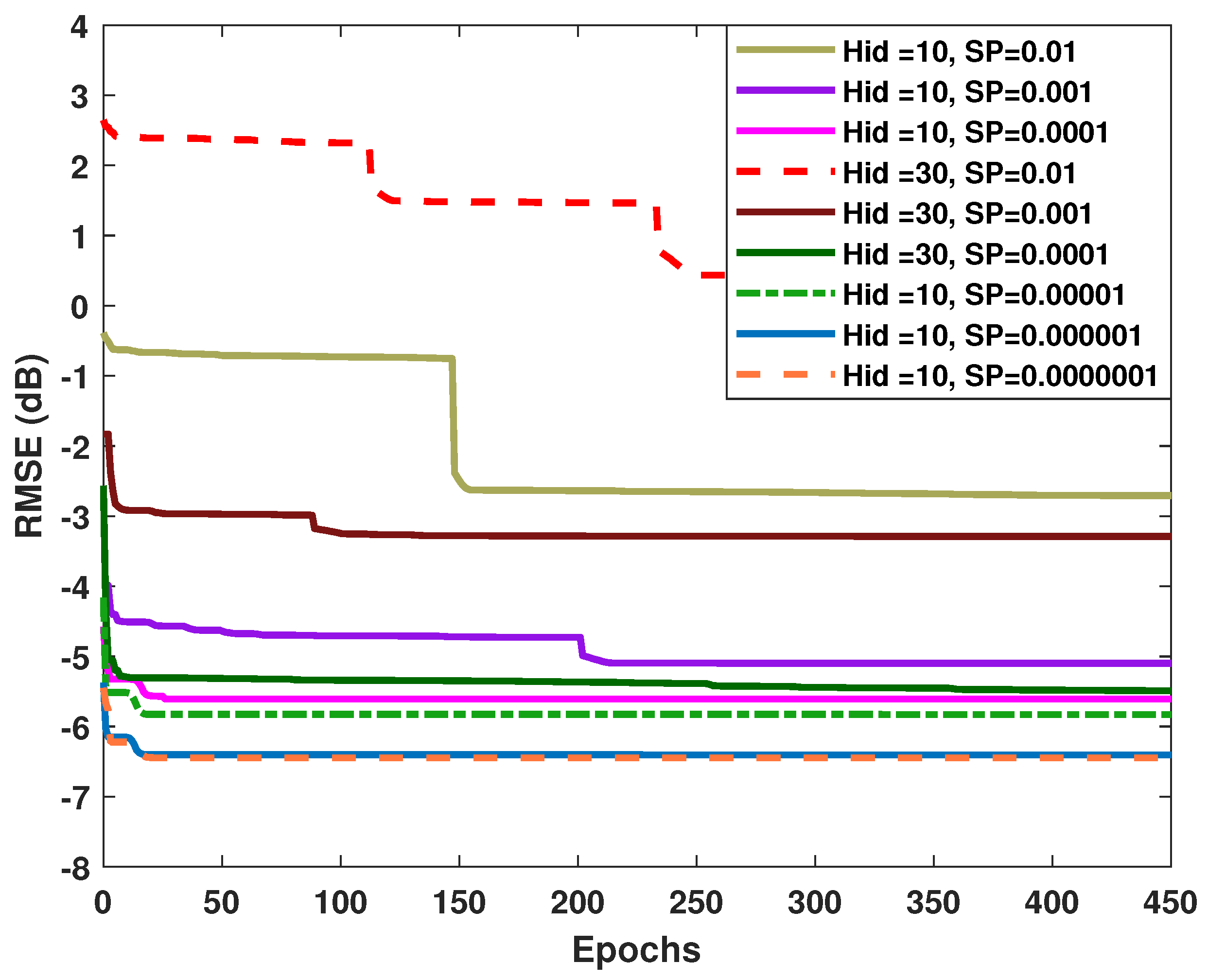
4.3. Convergence Results of the Proposed Algorithm

Figure 8 shows the root mean square error (RMSE) between the output of the proposed autoencoder neural network and its input versus the number of epochs. Specifically, the input is the designed p × p dimensional C r e r based on the processed and selected covariances, and the output is its reconstructed data C ^ r e r after the encoding and decoding by the proposed method. Large RMSE means relatively large differences between C r e r and C ^ r e r . It can be seen that the RMSE drops dramatically at about n e p = 100 to n e p = 250 epochs, and then, with the increased number of epochs, the RMSE remains unchanged. For different CNRs, the convergence of network training can be obtained by the proposed method. Once converged, more epochs are not helpful in improving the accuracy of the reconstruction.
Figure 9 illustrates the RMSE of the proposed network versus the number of epochs, where different numbers of hidden neurons and sparsity proportions are analyzed for comparison. Under different parameter settings, the proposed method can converge with a certain number of the hidden neurons. It can be observed in Figure 9 that the setting of s p = 0.0001 provides the lowest RMSE and the fastest convergence, which can be achieved when the number of epochs reaches just n e p = 5 to n e p = 30 . Additionally, with the same s p , the number of the hidden neurons H i d d e n s i z e = 30 leads to a higher RMSE than H i d d e n s i z e = 10 . For these reasons, a lower sparsity proportion encourages the higher degree of sparsity. Furthermore, within the proper limits, higher sparsity with lower s p and fewer hidden neurons force the proposed network to capture only the more important characteristics and be less sensitive to the deviations of the inaccurate samples. This is beneficial to a more accurate reconstruction of C r e r . With regard to the proper limits of the sparsity at this condition, as can be seen from Figure 9, when the proportion s p drops down to s p = 0.000001 , higher sparsity with lower s p cannot result in a better RMSE between the output of the proposed autoencoder network and its input. However, lower sparsity with s p = 0.01 is improper because of the corresponding large RMSEs. Therefore, 0.01 s p 0.000001 can be used to be the sparsity proportion for the proposed network.

4.4. Computation Time of the Proposed Algorithm

Figure 10 shows the computation time of the proposed method versus the total number of epochs n e p , with different parameter settings of p, H i d d e n s i z e , and s p . Moreover, the computation time of the other analyzed methods versus the number of the training samples L is also shown in Figure 10. Different from the other analyzed methods whose computation complexity is mainly affected by L, the computational burden of the proposed method mainly comes from the total number of epochs. In Figure 10, with the reduction of the epochs n e p , the speed is improved gradually and obviously. The setting of s p = 0.0001 acquires obvious advantages when the epochs n e p > 50 . Additionally, at the same s p , fewer dimensions of the designed C r e r and fewer hidden neurons can contribute to lowering the computation time of the proposed method. However, as can also be seen from Figure 10, compared with the DW, ADC, JDL, and STAP methods, the proposed method is obviously slower because of the network training for the reconstruction of clutter-plus-noise covariances.

5. Discussion

With the designed unique matrix, the proposed method compresses and retains the characteristics of the covariances and abandons the deviations caused by the deficiency of IID training samples. The design of the dimension p of the unique matrix in the proposed method is less than half of the DOF, that is p < N K / 2 . This is because, according to the properties of clutter-plus-noise covariances and the structure of CNCM, p < N K / 2 can ensure that the clutter-plus-noise power { R ^ X c n ( i , i ) } i = 1 , 2 , , N K located at the diagonal position is excluded from the selected covariances. This protects the most important power characteristics of CNCM and avoids the characteristic losses caused by the reconstruction process. Therefore, as the input of the network, the unique matrix with a certain dimension and matrix transformations allows the nonlinearity of the network be successfully explored and contributed to the improvement of CNCM.
Traditional dimension or rank reduction methods and distance compensation methods try to adapt to the inadequate IID training samples at the cost of reducing the degree of freedom of the system, giving up part of the sample data or relying on the inertial navigation system parameters. These disadvantages make the performance of clutter suppression and target detection not ideal and make the level of self-adaptability low. In contrast, the proposed method overcomes the above deficiencies, and it improves self-adaptability without reducing the degree of freedom. For different conditions of inadequate IID training samples, including the non-uniformity caused by the clutter range dependence of non-side-looking radar and the insufficient quantity, the proposed method provides obviously better clutter suppression performance. However, the proposed method has relatively high computational complexity, as shown in the simulations. The main cost of computing time is network training containing gradient descent process with iterations. As a result, DW, ADC, JDL, and STAP algorithms, which are without iterations, are faster than the proposed method. For further improvement of computing time, faster network training methods can be used to replace the gradient descent method. Moreover, controlling the total number of iterations can also make a contribution.

6. Conclusions

In this paper, we propose an autoencoder neural network-based STAP algorithm for airborne radar with inadequate training samples. In the proposed method, a matrix to be decoded and encoded whose dimension is less than half of the DOF is designed by processing of the selected clutter-plus-noise covariances. Then, by training the proposed autoencoder neural network and the invert processing for its output, the reconstruction of the clutter-plus-noise covariances is achieved for STAP. The simulation results have verified that the proposed method performs obviously superior clutter suppression for both side-looking and non-side-looking radars with strong clutter. Moreover, the proposed method can better adapt to the non-ideal sample conditions including the non-uniform clutter environments and inadequate training samples.

Author Contributions

Conceptualization, J.L. and G.L.; methodology, J.L.; software, J.L. and F.H.J.; resources, J.L., G.L., J.X. and C.Z.; writing—original draft preparation, J.L.; writing—review and editing, J.L. and J.X.; supervision, S.Z. and F.H.J.; funding acquisition, G.L., J.X., S.Z., J.L. and C.Z. All authors have read and agreed to the published version of the manuscript.

Funding

This work was supported by the National Natural Science Foundation of China (NSFC) under Grants 61901340, 61931016, and 62071344, the Young Talent Starlet in Science and Technology in Shaanxi under Grant No. 2022KJXX-38, the Fundamental Research Funds for the Central Universities under Grant JB210212, the Science and Technology Innovation Team of Shaanxi Province under Grant 2022TD-38, and the stabilization support of National Radar Signal Processing Laboratory under Grant KGJ202X0X.

Conflicts of Interest

The authors declare no conflict of interest.

References

  1. Kang, M.S.; Kim, K.T. Automatic SAR Image Registration via Tsallis Entropy and Iterative Search Process. IEEE Sens. J. 2020, 20, 7711–7720. [Google Scholar] [CrossRef]
  2. Gong, M.G.; Cao, Y.; Wu, Q.D. A Neighborhood-Based Ratio Approach for Change Detection in SAR Images. IEEE Geosci. Remote Sens. Lett. 2012, 9, 307–311. [Google Scholar] [CrossRef]
  3. Hakim, W.L.; Achmad, A.R.; Eom, J.; Lee, C.W. Land Subsidence Measurement of Jakarta Coastal Area Using Time Series Interferometry with Sentinel-1 SAR Data. J. Coast. Res. 2020, 102, 75–81. [Google Scholar] [CrossRef]
  4. Ward, J. Space-Time Adaptive Processing for Airborne Radar; Technical Report; MIT Lincoln Laboratory: Lexington, KY, USA, 1998. [Google Scholar]
  5. Klemm, R. Principles of Space-Time Adaptive Processing; The Institution of Electrical Engineers: London, UK, 2002. [Google Scholar]
  6. Guerci, J.R. Space-Time Adaptive Processing for Radar; Artech House: Norwood, MA, USA, 2003. [Google Scholar]
  7. Reed, I.S.; Mallett, J.D.; Brennan, L.E. Rapid convergence rate in adaptive arrays. IEEE Trans. Aerosp. Electron. Syst. 1974, AES-10, 853–863. [Google Scholar] [CrossRef]
  8. Zhang, Q.; Mikhael, W.B. Estimation of the clutter rank in the case of subarraying for space-time adaptive processing. Electron. Lett. 1997, 35, 419–420. [Google Scholar] [CrossRef]
  9. Melvin, W.L. Space-time adaptive radar performance in heterogeneous clutter. IEEE Trans. Aerosp. Electron. Syst. 2000, 36, 621–633. [Google Scholar] [CrossRef]
  10. Lapierre, F.D.; Ries, P.; Verly, J.G. Foundation for mitigating range dependence in radar space-time adaptive processing. IET Radar Sonar Navig. 2009, 3, 18–29. [Google Scholar] [CrossRef] [Green Version]
  11. Guerci, J.R.; Goldstein, J.S.; Reed, I.S. Optimal and adaptive reduced-rank STAP. IEEE Trans. Aerosp. Electron. Syst. 2000, 36, 647–663. [Google Scholar] [CrossRef]
  12. Liao, G.S.; Bao, Z.; Xu, Z.Y. A framework of rank-reduced space-time adaptive processing for airborne radar and its applications. Sci. China Ser. E Technol. Sci. 1997, 40, 505–512. [Google Scholar] [CrossRef]
  13. Zhang, L.; Bao, Z.; Liao, G.S. A comparative study of eigenspace based rank reduced STAP methods. Acta Electron. Sin. 2000, 28, 27–30. [Google Scholar]
  14. Goldstein, J.S. Reduced rank adaptive filtering. IEEE Trans. Signal Process. 1997, 45, 492–496. [Google Scholar] [CrossRef]
  15. Wang, W.L.; Liao, G.S.; Zhang, G.B. Improvement on the performance of the auxiliary channel STAP in the non-homogeneous environment. J. Xidian Univ. 2004, 20, 426–429. [Google Scholar]
  16. Wang, Y.; Peng, Y. Space-time joint processing method for simultaneous clutter and jamming rejection in airborne radar. Electron. Lett. 1996, 32, 258. [Google Scholar] [CrossRef]
  17. Yang, Z.C.; Li, X.; Wang, H.Q.; Jiang, W.D. On clutter sparsity analysis in space-time adaptive processing airborne radar. IEEE Geosci. Remote Sens. Lett. 2013, 10, 1214–1218. [Google Scholar] [CrossRef]
  18. Sun, K.; Meng, H.; Wang, Y.; Wang, X. Direct data domain STAP using sparse representation of clutter spectrum. Signal Process. 2011, 91, 2222–2236. [Google Scholar] [CrossRef] [Green Version]
  19. Yang, Z.C.; Lamare, R.; Liu, W. Sparsity-based STAP using alternating direction method with gain/phase errors. IEEE Trans. Aerosp. Electron. Syst. 2017, 53, 2756–2768. [Google Scholar]
  20. Ji, S.; Xue, Y.; Carin, L. Bayesian compressive sensing. IEEE Trans. Signal Process. 2008, 56, 2346–2356. [Google Scholar] [CrossRef]
  21. Lim, C.H.; Mulgrew, B. Filter banks based JDL with angle and separate Doppler compensation for airborne bistatic radar. In Proceedings of the International Radar Symposium India, Bangalore, India, 18–22 December 2005; pp. 583–587. [Google Scholar]
  22. Lapierre, F.; Droogenbroeck, M.V.; Verly, J.G. New methods for handling the dependence of the clutter spectrum in non-sidelooking monostatic STAP radars. In Proceedings of the IEEE Acoustics, Speech, and Signal Processing Conference, Hong Kong, China, 6–10 April 2003; pp. 73–76. [Google Scholar]
  23. Lapierre, F.; Verly, J.G. Registration-based range dependence compensation for bistatic STAP radars. EURASIP J. Appl. Signal Process. 2005, 1, 85–98. [Google Scholar] [CrossRef] [Green Version]
  24. Lapierre, F.; Verly, J.G. Computationally-efficient range dependence compensation method for bistatic radar STAP. In Proceedings of the IEEE International Radar Conference, Arlington, VA, USA, 9–12 May 2005; pp. 714–719. [Google Scholar]
  25. Borsari, G.K. Mitigating effects on STAP processing caused by an inclined array. In Proceedings of the 1998 IEEE Radar Conference, Dallas, TX, USA, 11–14 May 1998; pp. 135–140. [Google Scholar]
  26. Kreyenkamp, O.; Klemm, R. Doppler compensation in forward-looking STAP radar. IEE Proc. Radar Sonar Navig. 2001, 148, 253–258. [Google Scholar] [CrossRef]
  27. Himed, B.; Zhang, Y.; Hajjari, A. STAP with angle-Doppler compensation for bistatic airborne radars. In Proceedings of the IEEE Radar Conference, Long Beach, CA, USA, 25 April 2002; pp. 311–317. [Google Scholar]
  28. Pearson, F.; Borsari, G. Simulation and analysis of adaptive interference suppression for bistatic surveillance radars. In Proceedings of the Adaptive Sensor Array Process, Lexington, MA, USA, 5–6 June 2007; LincoIn Laboratory: VIrkshop, MA, USA, 2007. [Google Scholar]
  29. Liu, K.; Wang, T.; Wu, J.; Liu, C.; Cui, W. On the Efficient Implementation of Sparse Bayesian Learning-Based STAP Algorithms. Remote Sens. 2022, 14, 3931. [Google Scholar] [CrossRef]
  30. Xu, J.W.; Liao, G.S.; Huang, L.; Zhu, S.Q. Joint magnitude and phase constrained STAP approach. Digit. Signal Process. 2015, 46, 32–40. [Google Scholar] [CrossRef]
  31. Ottersten, B.; Stoica, P.; Roy, R. Covariance matching estimation techniques for array signal processing applications. Digit. Signal Process. 1998, 8, 185–210. [Google Scholar] [CrossRef]
  32. Bengio, Y.; Courville, A.; Vincent, P. Representation learning: A review and new perspectives. IEEE Trans. Pattern Anal. Mach. Intell. 2013, 35, 1798–1828. [Google Scholar] [CrossRef] [PubMed]
  33. Goodfellow, I.; Bengio, Y.; Courville, A. Deep Learning; MIT Press: Cambridge, UK, 2016; Volume 1, Chapter 14; pp. 499–507. [Google Scholar]
  34. Gregor, K.; Lecun, Y. Learning fast approximations of sparse coding. In Proceedings of the 27th International Conference on International Conference on Machine Learning, Haifa, Israel, 21–24 June 2010; pp. 399–406. [Google Scholar]
  35. Zhang, S.X.; Choromanska, A.; Yann, L.C. Deep learning with Elastic Averaging SGD. Adv. Neural Inf. Process. Syst. 2015, 28, 1–24. [Google Scholar]
Figure 1. Space-time distributions of clutter spectra with data of original STAP (left) and proposed method (right).
Remotesensing 14 06021 g001
Figure 2. (a) Space-time distributions of non-uniform clutter caused by non-side-looking array with data of original STAP and proposed method. (b) Space-time distributions of target and non-uniform clutter.
Remotesensing 14 06021 g002
Figure 3. Frequency response of space-time two dimensions for original STAP method (left) and proposed method (right).
Remotesensing 14 06021 g003
Figure 4. IF versus normalized Doppler frequency for non-side-looking radar.
Remotesensing 14 06021 g004
Figure 5. IF versus normalized Doppler frequency for different platform parameters.
Remotesensing 14 06021 g005
Figure 6. IF versus normalized Doppler frequency for side-looking radar.
Remotesensing 14 06021 g006
Figure 7. IF versus normalized Doppler frequency for CNR = 50 dB. (a) The number of training samples is L = 50 . (b) The number of training samples is L = 60 .
Remotesensing 14 06021 g007
Figure 8. RMSE between the output and the original input versus the number of epochs.
Remotesensing 14 06021 g008
Figure 9. RMSE of the proposed network versus the number of epochs for different hidden sizes and sparsity proportions.
Remotesensing 14 06021 g009
Figure 10. Computation time versus the total number of epochs.
Remotesensing 14 06021 g010
Table 1. Summary of the proposed method.
(1)
By matching filter processing and pulse stacking, the received data are obtained as Equation (1).
(2)
According to the space-time covariance, a unique matrix is proposed.
(a)
The dimension of the unique matrix is designed as less than half of the DOF as Equations (11)–(13);
(b)
A series of covariance data selections and matrix transformations are proposed, as Equations (14)–(16).
(3)
Designing the unique matrix as the input, the proposed method further constructs the autoencoder network for it with l 2 regularization and sparsity regularization.
(a)
The activation functions are obtained from Equations (17)–(20);
(b)
The loss function is obtained from Equations (21)–(26).
(4)
Training the proposed network by means of reducing the total loss function with gradient descent iterations as Equations (27)–(34).
(5)
Taking advantage of the designed structure of the unique matrix and the output of the proposed network, the inverse matrix transformation is brought in and covariances are reconstructed, as Equations (35)–(36).
(6)
Performing STAP with the reconstructed clutter-plus-noise covariances, clutter suppression can be achieved by Equations (7) and (8).
Publisher’s Note: MDPI stays neutral with regard to jurisdictional claims in published maps and institutional affiliations.

