Article

Retrieving Soil Moisture in the Permafrost Environment by Sentinel-1/2 Temporal Data on the Qinghai–Tibet Plateau

1
School of Geographical Sciences, Nanjing University of Information Science & Technology, Nanjing 210044, China
2
University of Chinese Academy of Sciences, Beijing 100049, China
3
Cryosphere Research Station on Qinghai-Tibet Plateau, State Key Laboratory of Cryospheric Sciences, Northwest Institute of Eco-Environment and Resources, Chinese Academy of Sciences, Lanzhou 730000, China
4
Department of Geography, Ludwig-Maximilians-Universität München, 80333 Munich, Germany
*
Author to whom correspondence should be addressed.
Remote Sens. 2022, 14(23), 5966; https://doi.org/10.3390/rs14235966
Submission received: 14 October 2022 / Revised: 19 November 2022 / Accepted: 21 November 2022 / Published: 25 November 2022

Abstract

:
Soil moisture (SM) products presently available in permafrost regions, especially on the Qinghai–Tibet Plateau (QTP), hardly meet the demands of evaluating and modeling climatic, hydrological, and ecological processes, due to their significant bias and low spatial resolution. This study developed an algorithm to generate high-spatial-resolution SM during the thawing season using Sentinel-1 (S1) and Sentinel-2 (S2) temporal data in the permafrost environment. This algorithm utilizes the seasonal backscatter differences to reduce the effect of surface roughness and uses the normalized difference vegetation index (NDVI) and the normalized difference moisture index (NDMI) to characterize vegetation contribution. Then, the SM map with a grid spacing of 50 m × 50 m in the hinterland of the QTP with an area of 505 km × 246 km was generated. The results were independently validated based on in situ data from active layer monitoring sites. It shows that this algorithm can retrieve SM well in the study area. The coefficient of determination (R2) and root-mean-square error (RMSE) are 0.82 and 0.06 m3/m3, respectively. This study analyzed the SM distribution of different vegetation types: the alpine swamp meadow had the largest SM of 0.26 m3/m3, followed by the alpine meadow (0.23), alpine steppe (0.2), and alpine desert (0.16), taking the Tuotuo River basin as an example. We also found a significantly negative correlation between the coefficient of variation (CV) and SM in the permafrost area, and the variability of SM is higher in drier environments and lower in wetter environments. The comparison with ERA5-Land, GLDAS, and ESA CCI showed that the proposed method can provide more spatial details and achieve better performance in permafrost areas on QTP. The results also indicated that the developed algorithm has the potential to be applied in the entire permafrost regions on the QTP.

1. Introduction

Soil moisture (SM) is an essential component of the terrestrial hydrological cycle ecosystem [1,2]. In ecology, SM affects the growth and activity of vegetation and microorganisms by controlling the division of water [3], and can also mitigate changes in soil organic carbon content caused due to climate warming [4]. In hydrology, SM is not only an important parameter of the water cycle but is also used to infer surface- and ground-water exchanges [5]. In climatology, SM affects regional climate through changing surface albedo, evapotranspiration intensity, and sensible and latent heat fluxes [6]. In the permafrost environment of the Qinghai–Tibet Plateau (QTP), the SM in the active layer is significantly altered by the seasonal freezing and thawing processes and influences the energy exchange between permafrost terrain and the atmosphere [7,8]. The accurate information on the spatial and temporal distribution of SM helps advance hydrological, ecological, and climatological studies in permafrost areas [9].
In the permafrost area of 1.06 × 10⁶ km2 of the QTP [10], it is critical for various scientific studies to obtain accurate spatial distribution data of SM on a large scale. Due to the harsh environment and inconvenience of accessing the QTP, the traditional methods of obtaining SM by sampling measurement and monitoring are limited. Several meteorological and hydrological stations have been deployed over the past few decades, and data scarcity has been filled to a degree [11]. These restricted sites are unevenly distributed on the edge of permafrost areas or on seasonally frozen ground areas, which makes it challenging to study SM with high spatial heterogeneity [6,12]. Remote sensing technology has achieved significant advances in SM monitoring, with its unique large-area observation capabilities, and some remote sensing products and reanalysis data have been produced, such as the fifth generation of the land component of the European Centre for Medium-Range Weather Forecast atmospheric reanalysis (ERA5-Land) [13], the European Space Agency Climate Change Initiative (ESA CCI) [14], and the Noah land surface model driven by Global Land Data Assimilation System (GLDAS-Noah) [15]. Xing et al. evaluated seven SM data products (SMAP, SMOS-IC, ASCAT, ERA5-Land, ESA CCI, LPRM, AMSR2) over the permafrost region of the QTP based on in situ SM measurements and found that the SM data of ESA CCI had the highest accuracy [16]. Due to the lack of adequate measurement data, SM products generated by the model assimilation are significantly biased in the QTP [17]. In addition, the SM product data at a spatial resolution of tens of kilometers are affected by mixed pixels and do not accurately describe the SM distribution. The coefficient of variation (CV) analysis is often used to describe significant patterns in regional mean SM content, with the relationship between CV and SM often showing a hysteresis pattern in spatial variability [18,19,20]. The spatial–temporal SM variations have never been revealed over the permafrost area in the QTP, where the relationship between the CV and mean SM is similar to that found in other regions is unclear [21,22]. The lack of high-spatial-resolution SM data in the permafrost region of the QTP greatly limits the studies of the spatial–temporal distribution characteristics of SM. Few studies are able to analyze the spatial–temporal variations of SM in permafrost areas on a fine scale.
Synthetic Aperture Radar (SAR) has proven its high potential for retrieving high-spatial-resolution SM using the backscatter coefficient (σ°) [23,24]. Some empirical [25,26], semi-empirical [27], and physical scattering models [28] have been developed to relate backscattering with surface SM, roughness, and vegetation. Surface scattering models are commonly used for bare soil including the semi-empirical Dubios model [29], the Oh model [30], and the physically based Integrate Equation Model (IEM) [31]. These are usually integrated with vegetation scattering models, such as semi-empirical water cloud models (WCM), to predict scattering from vegetated areas [32,33]. Studies have developed algorithms for retrieving SM based on IEM or WCM inversion using minimization, LUT, and machine learning approaches. In 2014, He et al. estimated SM in the alpine meadow region by coupling the IEM and the WCM with R2 and RMSE reaching 0.71 and 0.03 m3/m3, respectively [34]. In 2017, Bai et al. first estimated SM in the alpine steppe region of Magu using Sentinel-1 (S1) data with the WCM [35]. In 2021, Yang et al. coupled the improved Oh model in 2004 and WCM to estimate SM in the Nagqu region based on S1 data and MODIS optical data with the assumption of constant surface roughness [36]. Despite the significant advance in scattering modeling, SM inversion from these microwave scattering models are commonly ill-posed and complicated [37,38]. Besides utilizing microwave scattering, several algorithms have been successively developed and widely used to retrieve SM, such as change detection (CD) and neural network (NN) [39,40,41]. NN are mathematical models that are commonly trained by vegetation coefficients, backscatter coefficients, and other parameters in studies of SM retrieval using SAR data, which have high requirements for the data volume. However, the NN method requires a large amount of data for training and validation, which greatly limits its application in the permafrost region of the QTP. The principle of the CD algorithm is based on the assumption that by differencing the backscattering coefficients in two periods, the effect of soil roughness and vegetation is reduced, and the backscatter difference is mainly due to the changes in SM [39]. Thus, it is more suitable than the NN algorithm for permafrost areas where a large amount of training data acquirement is difficult. Gao et al. mapped SM distributions at a 100 m spatial resolution located in Urgell using a CD algorithm by combining S1 and Sentinel-2 (S2) data [40]. Bauer-Marschallinger et al. used the CD algorithm to build the first global SM dataset with 1 km spatial resolution, which greatly advanced the progress of SM studies [42]. Zhu et al. proposed an unsupervised CD method as a pre-processing procedure for multi-temporal retrieval and improved the accuracy of the CD algorithm by reducing the uncertainty caused by changes in vegetation and roughness [43,44].
Over the QTP, studies of SM retrieval using SAR data have also been conducted in recent years. Yang et al. and Bai et al. estimated SM in alpine grassland environments in Nagqu and Magu, respectively, both with favorable results [35,36]. In the Beiluhe, Zhang et al. used estimated SM in alpine meadows and alpine deserts and improved the accuracy of estimating SM by the WCM and CD algorithms [45]. However, these SM retrieving studies on the QTP were conducted outside or in the margin/border of the permafrost area or within a very small permafrost region. The study area was very small, i.e., covering only a few square kilometers, and the effectiveness and accuracy of the retrieving algorithms or models were not tested in other areas. To our knowledge, no SM retrieving study has yet been conducted on the large-scale hinterland permafrost regions.
The freeze–thaw cycle of active layer soils and the water barrier of the frozen layer in the permafrost area play an active role in determining vegetation growth and SM retention [46,47]. It implies that in areas with high SM, the vegetation cover has significant interference with the radar signal. The vegetation canopy complicates the extraction of underlying soil water, as the canopy contains water and can also block or scatter radar signals [48]. Therefore, in the retrieval process, vegetation is another important factor that affects the radar signal in addition to SM. In the many ecological, hydrological, and agricultural studies, the vegetation canopy is usually expressed by the vegetation indices, such as Leaf Area Index (LAI), Normalized Difference Vegetation Index (NDVI), and the Enhanced Vegetation Index (EVI), biomass, vegetation height, etc. [35,45,49,50,51,52]. Several studies have shown that NDVI is easier to derive and has fewer errors than other vegetation indices and is widely used in SM retrieval studies [50,53]. In addition, in partially vegetated areas, Bao et al. found that Normalized Difference Moisture Index (NDMI) can also perform well in SM retrieval studies based on S1 data [54].
In the permafrost region on the QTP, the ground has a distinct freeze–thaw cycle process. The soil water is in a liquid state during summer and in a state of combination of ice and unfrozen water in other seasons [9]. The real implication of SM values obtained by in situ monitoring and sampling drying measurements could be different. In situ monitoring measures the unfrozen water (liquid water) content by monitoring the dielectric constant in the soil, such as the Hydra soil moisture sensor. The field-oven sampling acquires the total soil water content (unfrozen water and ice) by collecting in the field and then calculating the volumetric water content from the wet and dry weight of the soil. Meanwhile, σ° is sensitive to unfrozen soil water, and the frozen part is neglected in the retrieval process. The σ° could not represent the gross soil water content in all seasons except for the thawing season. Therefore, we need to be careful when choosing field “SM” data in developing and training SM retrieving algorithms [55].
In summary, a retrieval algorithm for SM is urgently needed to obtain SM spatial data which could promote hydrological, ecological, climatic, and engineering studies in the permafrost region of the QTP. In this study, the hinterland of the QTP was selected for SM retrieval, where a variety of surface types are included. The retrieval algorithm is trained and validated using multi-year in situ observations of different surface environments. We chose the months of July and August as the study period, which can reduce the errors caused by the freeze–thaw process of the soil. The SM retrieval during the thawing season could represent the gross soil water content. In addition, the CD algorithm is a promising method for SM retrieval in the permafrost region where a priori knowledge is scarce [39,40]. The liquid soil water is very small in the coldest winter season, by reference to the CD algorithm, the effect of surface roughness is minimized. Then, the vegetation effect is further represented and reduced by vegetation indexes (NDVI, NDMI) from optical data. Finally, the objectives of this study are: (1) to develop an SM retrieval algorithm suitable for permafrost environments on the QTP using high spatial-resolution SAR data to obtain spatial data of SM for the thawing season; and (2) to explore the spatial–temporal distribution characteristics of SM on the large extent of permafrost region on the QTP.

2. Materials and Methods
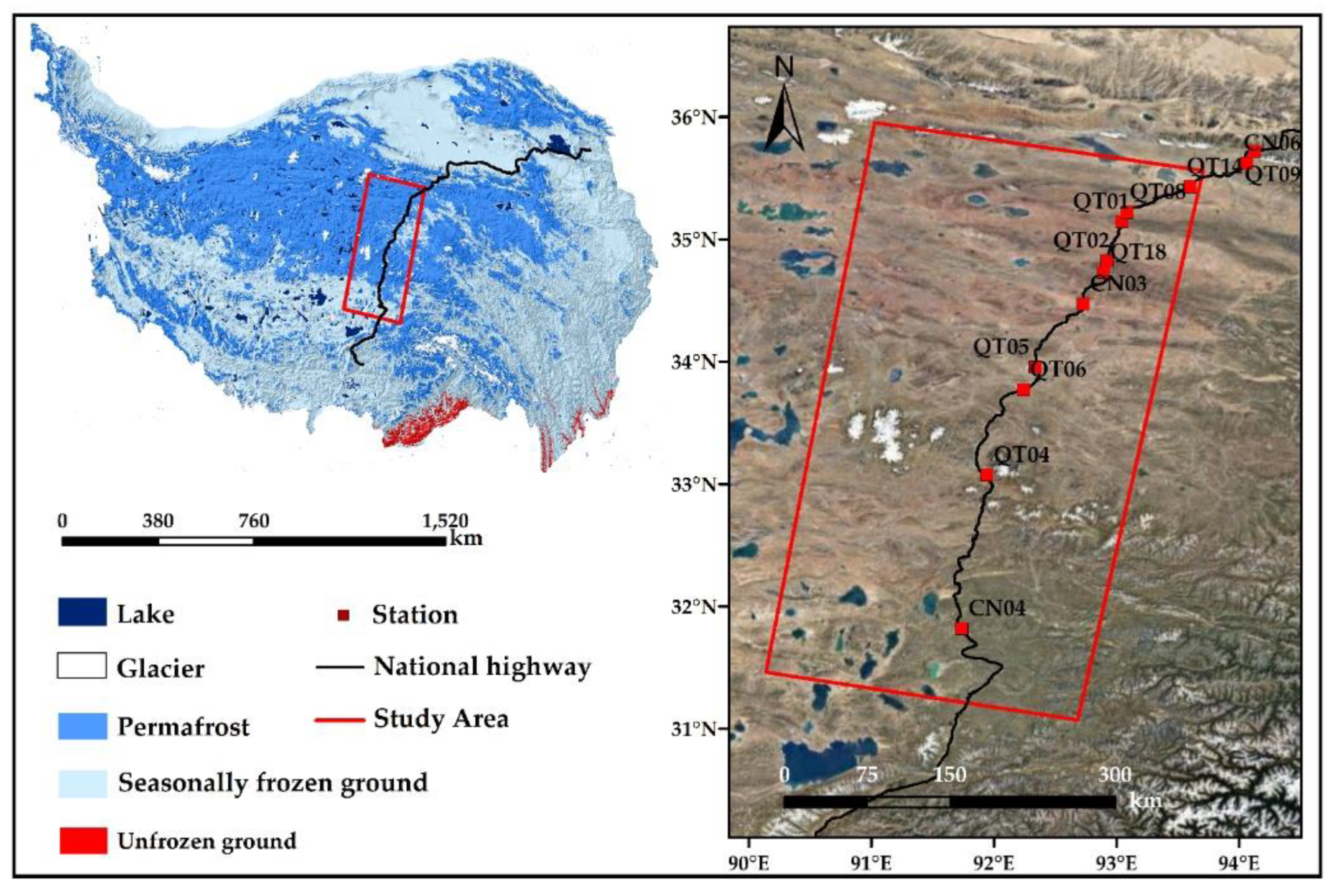
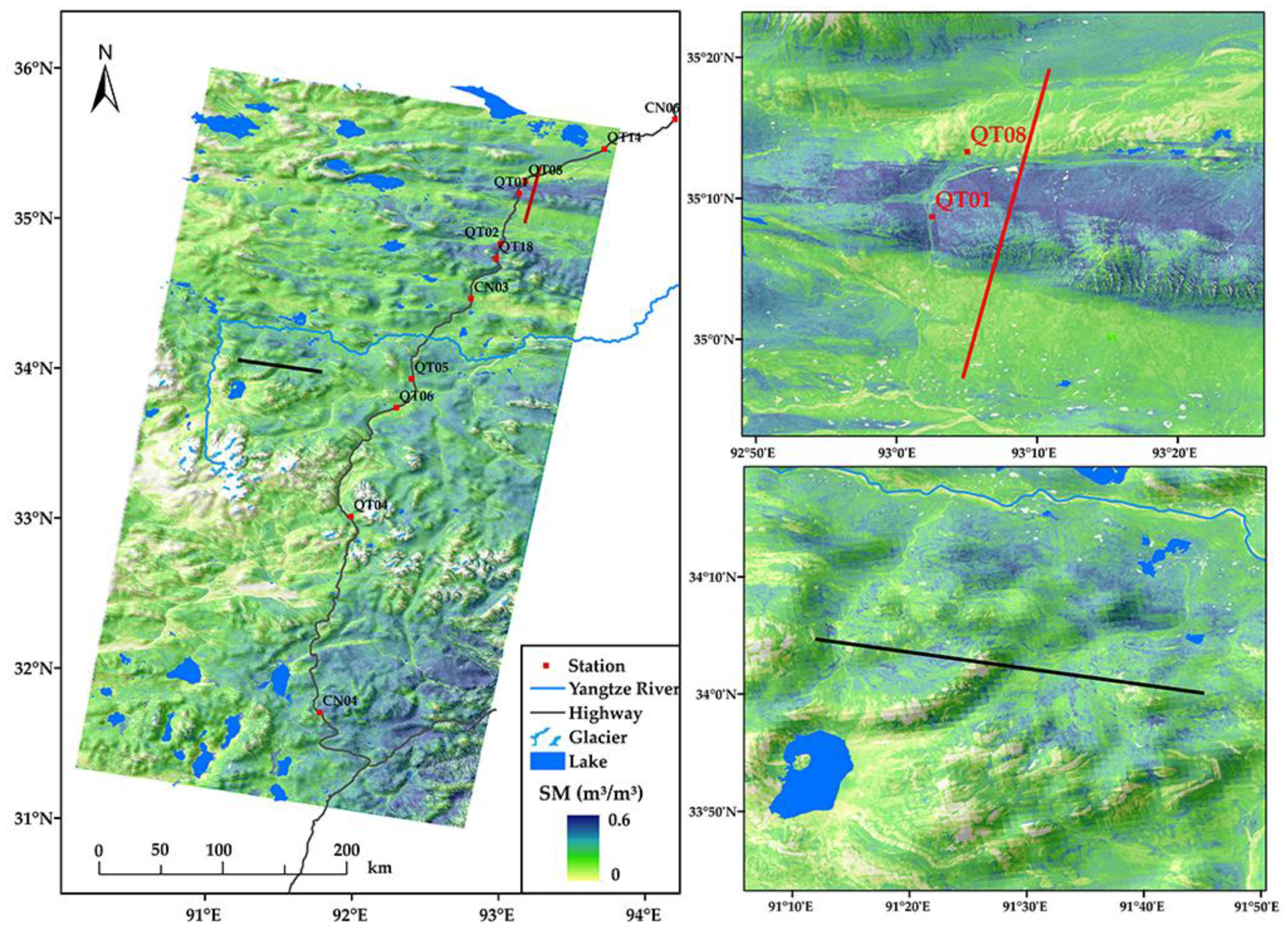
2.1. Study Area

In this study, an area of 505 km × 246 km in the hinterland of QTP along the Qinghai–Tibet Highway was selected as the study area, as shown in Figure 1. This area covers most of the stations of the SM and temperature monitoring of the permafrost networks [11]. The study area includes typical permafrost regions and seasonally frozen ground regions with an altitude between 4189 m and 6402 m a.s.l. The average annual temperature in this region is between −5.8 °C and −2.4 °C, and the trend of temperature increase is consistent, with an average rate of change of about 0.05 °C/a. The annual precipitation is in the range of approximately 210–580 mm, with sizeable interannual variation [56,57]. The precipitation is mainly concentrated between May and September, and there is an apparent upward fluctuation in annual precipitation, with an average variable rate of 7.49 mm/a from 2004 to 2016 [58].
The vegetation types in the study area are classified as alpine swamp meadows, alpine meadows, alpine steppes, and alpine deserts. The alpine meadows cover the largest areas, followed by alpine steppes and alpine swamp meadows at the least [59]. The degradation of the permafrost has affected the ecological situation in the QTP. The vegetation ecosystem degradation is significant, mainly manifested as the degradation of alpine swamp meadow to the alpine meadow and alpine meadow to alpine steppe [59].
The frozen ground undergoes seasonal freeze–thaw cycles [8]. On the QTP, the thawing process begins in mid-to-late May and lasts until late September to early November each year [58,60,61]. The effect of water transport during soil freezing and thawing on SM distribution is very significant. The measured data in the in situ show that the SM in the thawing season varies roughly between 0.1 m3/m3 and 0.5 m3/m3. When the soil is frozen in winter, the unfrozen water content is low.

2.2. Datasets

2.2.1. In Situ Observations

The in situ SM measurements are acquired from the SM and temperature observation network built by the Chinese Academy of Sciences (CAS) [11]. SM was measured by a Hydra soil moisture sensor and recorded by a CR10X/CR1000/CR3000 data logger, with an accuracy of ±2.5%. Table 1 shows detailed information on the stations used in the study. The elevation of these stations ranges from 4468 m to 5100 m a.s.l and spans about 420 km from north to south. The sites also contain several typical vegetation types of the QTP, including alpine swamp meadows, alpine meadows, and alpine steppes. They could represent the varied permafrost environment on the QTP to some extent. We collected 129 in situ SM data during the thawing season (months July, and August) from 2016 to 2019 at these sites, of which 100 were used for training the model and 29 for validation.

2.2.2. Sentinel-1

The Sentinel-1 (S1) satellites were launched by the European Space Agency (ESA) in the frame of Europe’s Copernicus program, including Sentinel-1A (S1A) and Sentinel-1B (S1B). The orbital period of S1A is 98.6 min, the revisit period is 12 days, and the combined AB satellite is 6 days. The interferometric wide (IW) imaging model with a spatial resolution of 5 m × 20 m provides a more accurate σ° and better meets the needs of this study [50].
We use the ground range detection (GRD) products of S1 in IW acquisition mode with the VV and VH polarizations from Google Earth Engine (GEE). Compared to the VH polarization of S1, the VV polarization has greater potential for SM retrieval [40,65,66,67]. Some researchers have used both VV and VH in SM retrieval studies and characterized the effect of vegetation by the ratio of VV and VH [41,68]. However, in the study, only VV single polarized data is acquired before February 2017. Therefore, the optical vegetation index NDVI is used in this study for characterizing vegetation. The backscattered images of VV polarization in the completely thawed season (months July, and August) and the completely frozen season (January to February) from 2016 to 2019, in a total of 89 acquisitions, are employed for the SM retrieval algorithm development and validation.

2.2.3. Sentinel-2

Sentinel-2 (S2) is a high-resolution imaging satellite that carries a multi-spectral imager (MSI). The revisit period for one satellite is 10 days, and the revisit period for two satellites is 5 days [69,70]. In this study, cloud-free S2 TOA Level-1C data one week before and after the S1 acquisition is selected to calculate vegetation and water indices using the green band (B3: Green), red band (B4: Red), near-infrared band (B8: NIR), and short-wave infrared (B11: SWIR) [71].

2.2.4. SRTM DEM

Shuttle Radar Topography Mission (SRTM) data is mainly measured jointly by the National Aeronautics and Space Administration (NASA) and the National Imagery and Mapping Agency (NIMA). Interferometric radar data is captured using dual radar antennas and converted into digital terrain data. This study uses the “NASA SRTM Digital Elevation 30-m” elevation dataset provided by the GEE platform [64].

2.2.5. SM Data Products
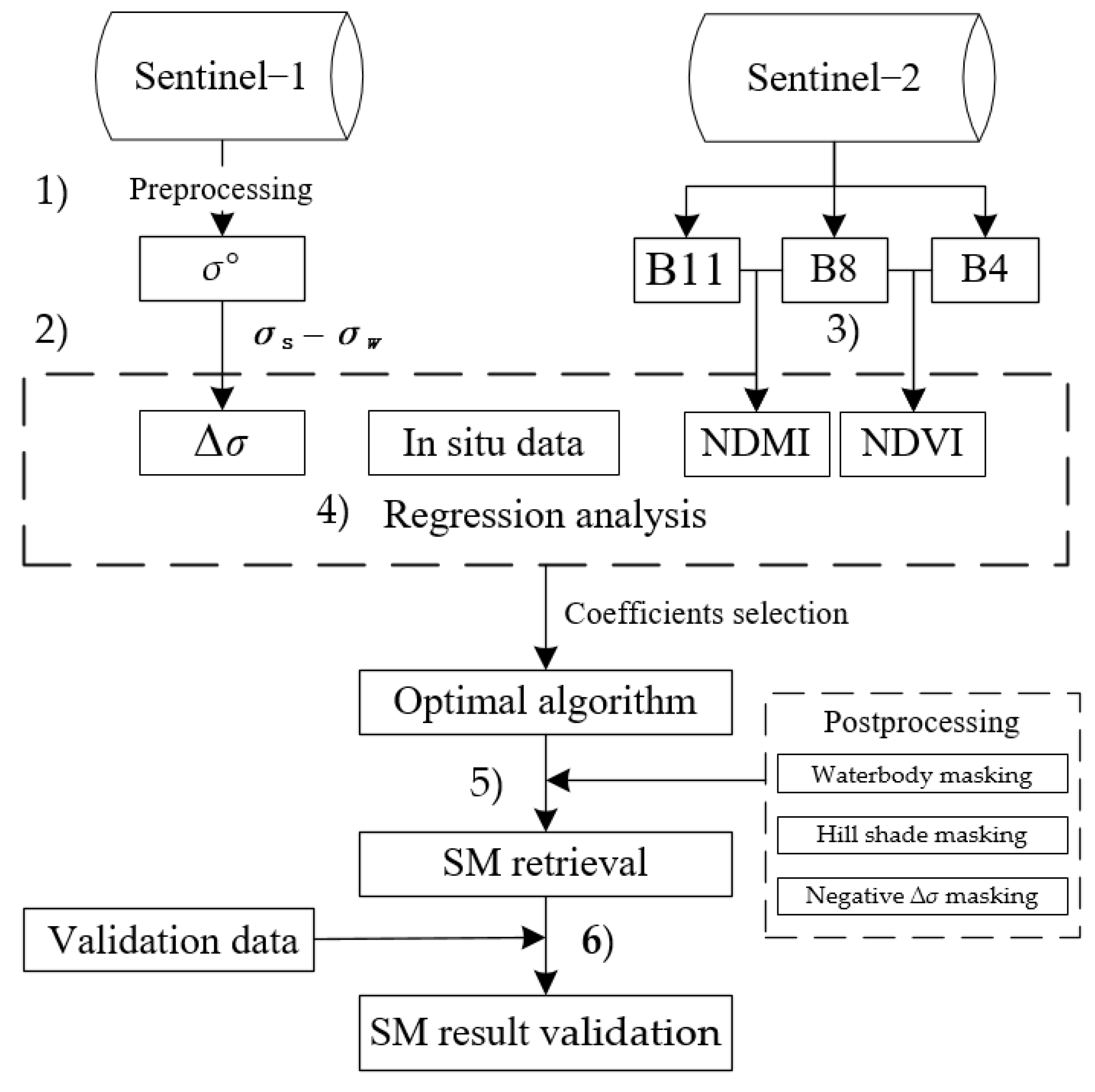
In this study, we also compared the retrieval SM with three SM data products, such as the fifth generation of the land component of the European Centre for Medium-Range Weather Forecasts atmospheric reanalysis (ERA5-Land) [13], the Noah land surface model driven by Global Land Data Assimilation System (GLDAS-Noah) [15], and the European Space Agency Climate Change Initiative (ESA CCI) [14]. The specific information of the three datasets and the first layer of the depth range are shown in Table 2. In this study, the SM product data for 2 July and 19 August 2018 were selected for comparing the spatial distribution and average SM content with the retrieval results.

2.3. Methods

The workflow of the SM retrieval algorithm development is illustrated in Figure 2. The main steps are summarized as (1) S1 backscatter preprocessing; (2) Reducing the effect of surface roughness; (3) Reducing the effect of vegetation; (4) SM retrieval algorithm construction; (5) SM result post-processing; and (6) Retrieval result validation.

2.3.1. S1 Backscatter Preprocessing

Data preprocessing was performed on the GEE platform [72]. GEE has performed some preprocessing of the S1 data using the ESA S1 Toolbox (S1TBX), including applying orbit files, removing thermal noise, removing GRD border noise, radiometric calibration, and Range-Doppler terrain correction. Furthermore, the S1 incident angle normalization and spatial filtering are needed to make the data as correct as possible.
  • S1 incident angle normalization
The σ° is affected by the incidence angle (θ0) of S1 and has a slight deviation from the actual situation. There is a certain correlation between θ0 and σ°, which can be expressed as a slope β [73,74]. This study chose the central incidence angle of the study area (38°) as the reference angle to reduce the overall error caused by extrapolation [42]. Therefore, as shown in Equation (1), we uniformly correct the σ to the value corresponding to the incident angle of 38° (σ° (38°)).
σ°(38°) = σ° (θ0) − β (θ0 − 38°) [dB].
The calculation of Equation (1) can be performed on the GEE.
  • Refined Lee Filtering
In order to reduce the speckle noise in the image while preserving the image edge information, the Refined Lee filter with a window size of 7 × 7 is used in this study [75,76].

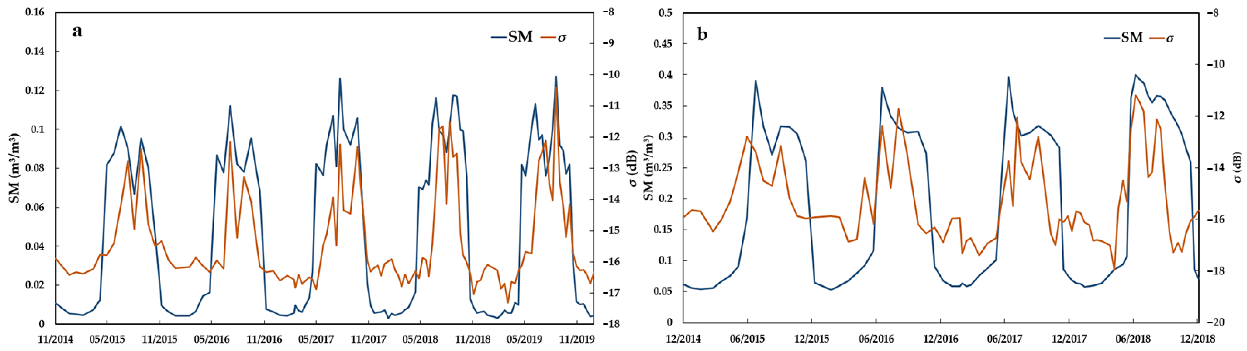
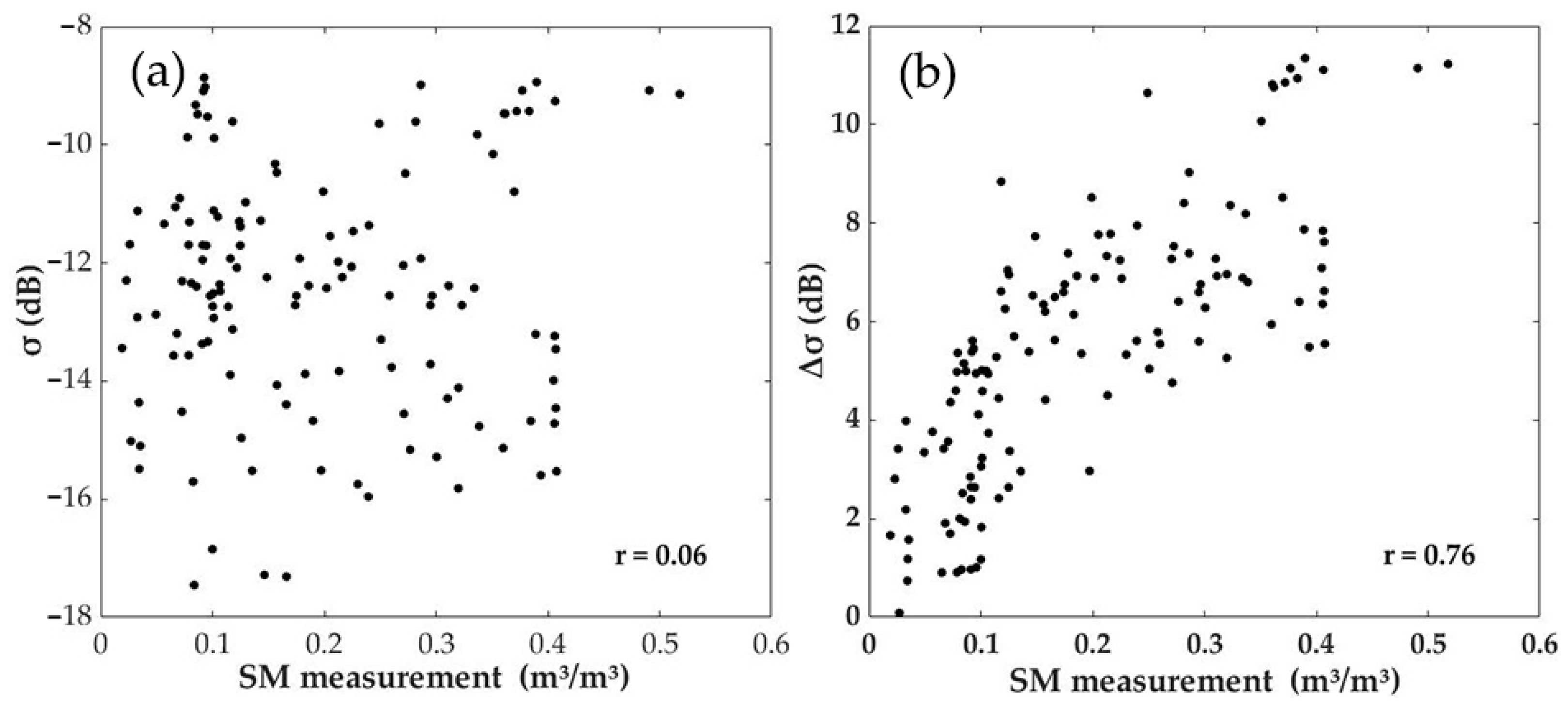
2.3.2. Sensitivity of Backscattering Coefficient to Soil Liquid Water

The correlation between SM and σ° in the permafrost region was analyzed at sites QT08 and QT09. As shown in Figure 3, the σ° and SM at both stations showed obvious seasonal variations, i.e., high in summer and low in winter. When the soil freezes, the soil’s liquid water content decreases sharply, and therefore, the dielectric constant decreases, and consequently, the σ° drops significantly.
Figure 3 also revealed that the same σ° corresponded to different SM values at the two sites. At site QT08, the σ° was in the range of −17 to −10 dB, corresponding to SM of about 0.003 to 0.13 m3/m3, while at site QT09, the σ° range was −17 to −11 dB, corresponding to the SM range of about 0.05 to 0.4 m3/m3. This shows that the range of σ° does not vary much between the two sites, but the corresponding SM ranges are dramatically different. Many studies have demonstrated that surface roughness and vegetation are the major factors affecting the correlation between surface backscatter intensity and SM [77]. Therefore, it is critical to reduce the effects of surface roughness and vegetation in the retrieval process to improve accuracy.

2.3.3. Reducing the Effect of Surface Roughness

The CD algorithm originally proposed by Wagner et al. determines the SM by linearly scaling the observed backscatter between that at the driest and wettest conditions [78]. The algorithm has been validated and used in many regions in SM retrieval studies in recent years, including semi-arid areas and mountainous areas [42,79]. Rignot EJM et al. conducted experiments in a mountainous region of the Katmai National Park and Preserve in Alaska and found that the CD algorithm is effective in removing the topographic influences [80]. Therefore, this study refers to the principle of the CD algorithm to eliminate the effect of topography in permafrost areas.
According to the characteristics of soil liquid water in the permafrost regions of QTP, the soil surface is mostly frozen in winter and holds little liquid water. Meanwhile, due to low precipitation during the period of January–February, the snowmelt or wet snowfall effect is limited, and the change in surface roughness in winter is not significant compared to the melting season. We assumed that the smallest σ° in winter of its temporal curves could represent the lowest liquid water content of the soil during this period. Therefore, we took the smallest value of σ° in the freezing season (January, February) as the reference value and subtracted it from the backscatter signal during the thawing season. The backscatter difference (Δσ) between the freezing and thawing seasons (months July, and August) represents the changes in SM and vegetation. It can be expressed as:
Δσ = σsσw
where σs is the σ° of the thawing season, and σw is the σ° of the freezing season. Figure 4 shows the distribution and details of σs, σw, and Δσ in the study area. In the case of Figure 4a,b, the topographic factor has a significant effect on the backscattered signal. Figure 4c shows that the method of calculating the σ° difference between summer and winter is effective in weakening this effect.

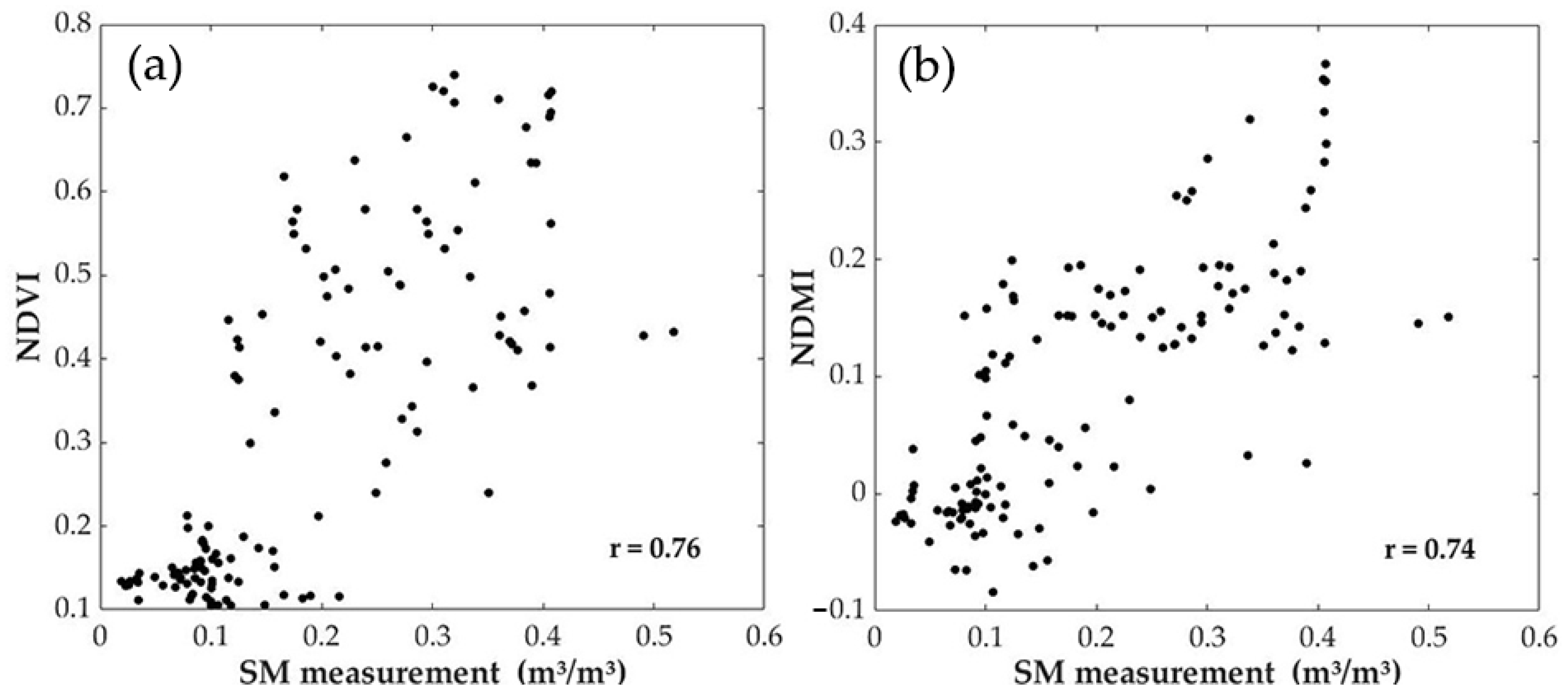
2.3.4. Reduce the Effect of Vegetation

We applied NDVI and NDMI to reflect vegetation characteristics and the water content in vegetation and proposed to use the combination of NDVI and NDMI to characterize the effect of vegetation on the σ. These vegetation indices were calculated as follows:
NDVI = (ρnir − ρred)/(ρnir + ρred)
NDMI = (ρnir − ρswir)/(ρnir + ρswir)
where ρred, ρnir, and ρswir are the reflection value in the red spectrum, the near-infrared spectrum, and the shortwave infrared spectrum, respectively. It is noteworthy that the contribution of soil to NDMI is primarily negative for some areas, while the contribution of green vegetation is mostly positive [81].

2.3.5. SM Retrieval Algorithm Construction

We collected 129 datasets (in situ data, and corresponding Δσ, NDVI, NDMI) during the thawing season (months July and August) from 2016 to 2019. A multiple linear regression model was constructed based on the linear relationship between SM and the Δσ, NDVI, and NDMI, and the SM retrieval algorithm can be expressed as follows:
SM = a × △σ + b × NDVI + c × NDMI + d
where a, b, and c are the coefficients of the three variables (△σ, NDVI, NDMI), respectively, and d is a constant. In order to ensure the universality of the retrieval algorithm, we arrange the in situ data of different years together and then performed 10,000 random divisions with a ratio of nearly 8 to 2 for determining the optimal coefficient. One part is used to obtain model coefficients (a, b, c, d). The other is used to verify the accuracy of retrieved SM. Thus, we can obtain 10,000 sets of coefficients, training, and validation of R2. Finally, we calculate the sum of R2 for training and validation processes using their sample size as the weights. The coefficients corresponding to the maximum sum of R2 are determined as the optimal coefficient.

2.3.6. SM Result Post-Processing

There are some outlier regions in the retrieval results, which are removed in the post-processing steps.
  • Waterbody masking
The sensitivity of the σ° to soil liquid water is its advantage of SM retrieval, but σ° will present an anomaly and deviate from the normal range when the sensor scans water bodies such as rivers and lakes. The normalized difference water index (NDWI) is calculated using the green band, and the near-infrared band can effectively identify the water body information [82]. The NDWI is calculated as follows:
NDWI = (ρgreen − ρnir)/(ρgreen + ρnir)
In Equation (6), ρgreen is the reflection in the green spectrum, corresponding to the B3 band of the S2. Then, a mask is created with 0 as the threshold to remove the water body part of the retrieved results.
  • Shadow masking
It is found that the σ° in the hillside or foothills usually shows outliers in our study area due to the radar signal being obscured and distorted in these areas. The local incidence angle (θ) can be calculated by using the zenith angle and azimuth angle of S1 to represent the illumination condition of the radar signal, expressed in Equation (7),
cosθ = cosθza × cosS + sinθza × sinS × cos(θaaA)
where θza is the zenith angle, which is the same angle as θ0, θaa is the azimuth angle, S is the slope, and A is the aspect. The pixels with θ smaller than a threshold to be defined are masked out. According to a visual comparison of shadow outliers and local incidence masks, the threshold of 15° is adopted in our study.
  • Negative ∆σ masking
Theoretically, there is a positive correlation between the σ° and the SM, and the σ° in the thawing season should be higher than that in winter. Hence, the area where the ∆σ is less than zero is considered abnormal and masked out during the post-processing.

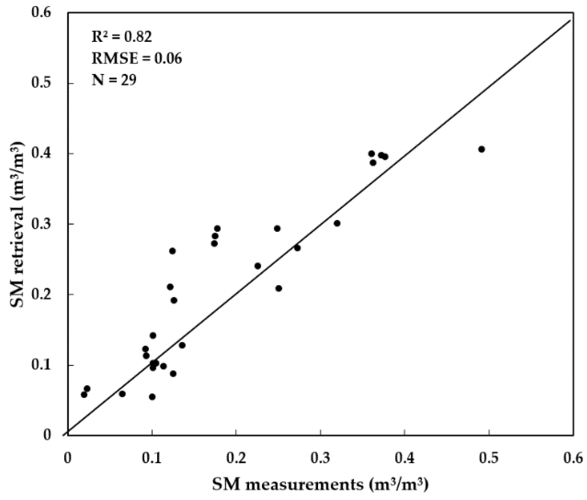
2.3.7. SM Retrieval Algorithm Validation

In all, 29 samples were used to evaluate the accuracy of the retrieved SM using the proposed algorithm. The root-mean-square error (RMSE) and coefficient of determination (R2) are applied to indicate the accuracy of the SM retrieval result.

3. Results

3.1. Reduce the Effects of Surface Roughness and Vegetation

Figure 5 shows the correlation of σ° and Δσ with the SM observations. There is no apparent correlation between the original σ° and SM, with a Pearson correlation coefficient (r) of 0.06. However, after subtracting the winter reference σw, the r between Δσ and SM reached 0.76. In Figure 5a, the sensitivity of the radar signal to SM is weakened by the effect of surface roughness. The comparison of SM with σ° and Δσ has proven that our method is able to reduce the effect of surface roughness and essentially improve the sensitivity of radar signals to SM.
NDVI and NDMI jointly characterize the contribution of vegetation to the retrieval of SM. As shown in Figure 6, NDVI and NDMI have high correlations with SM, with r of 0.76 and 0.74, respectively. The results indicate that NDVI and NDMI are suitable for characterizing the vegetation contribution in σ° of the study area.

3.2. SM Retrieval Algorithm and Validation

Table 3 lists the model coefficients and R2 value of 10,000 regressions. The coefficients which generate the highest weighted R2 were set as the optimal coefficients. The SM retrieval algorithm is expressed as follows:
SM = 0.02 × ∆σ + 0.24 × NDVI + 0.28 × NDMI + 0.003
As illustrated in Table 3 and Figure 7, the retrieved result is satisfactory, with R2 and RMSE reaching 0.82 and 0.07 m3/m3, respectively. As shown in Table 3, the mean values of the 10,000 sets of regression coefficients are very close to the optimal values, and the standard deviation is also relatively small. It indicates that the model coefficients are relatively stable, and not largely influenced by different divisions of training and validation samples, which demonstrates the robustness of the model.

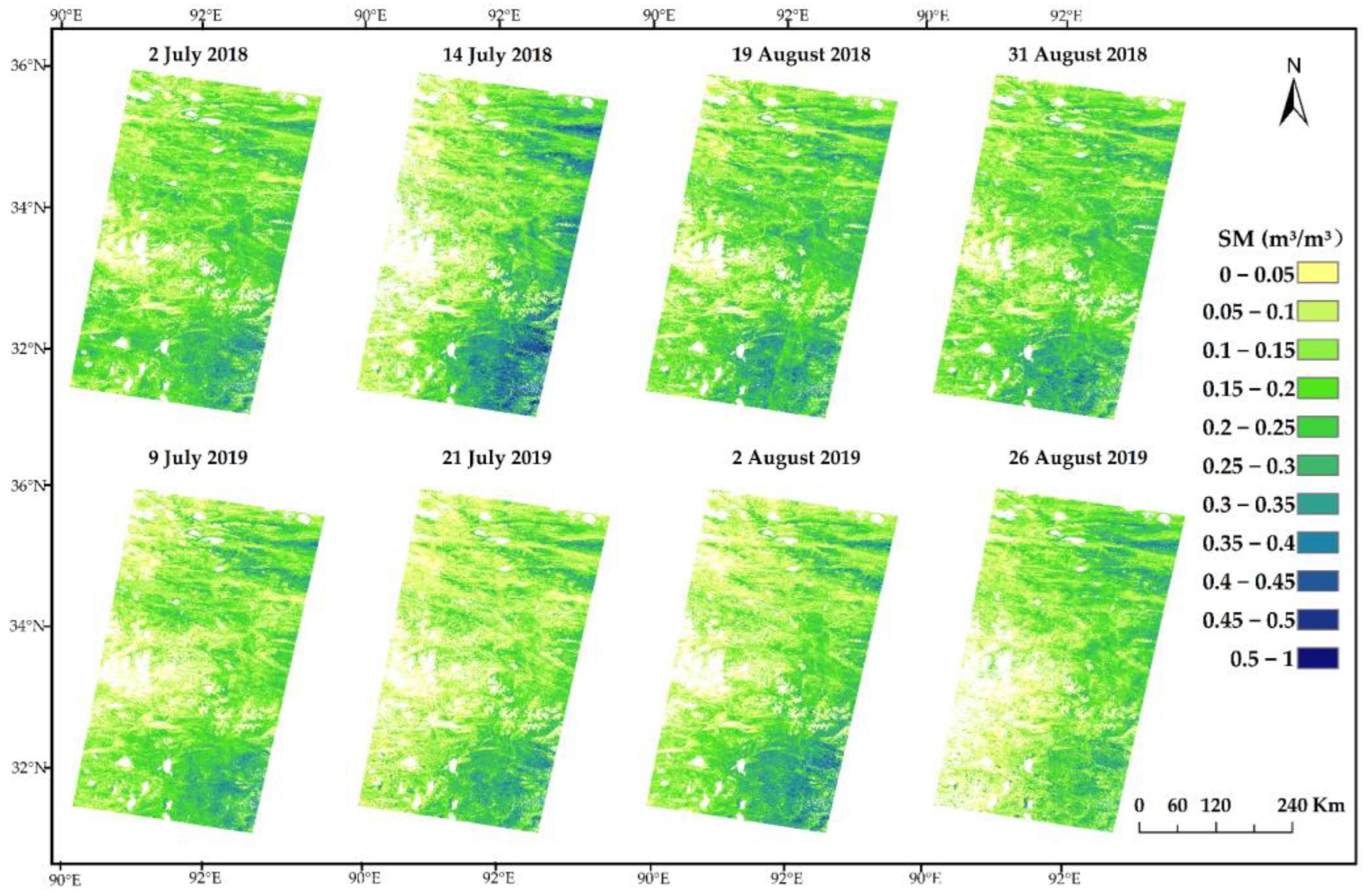
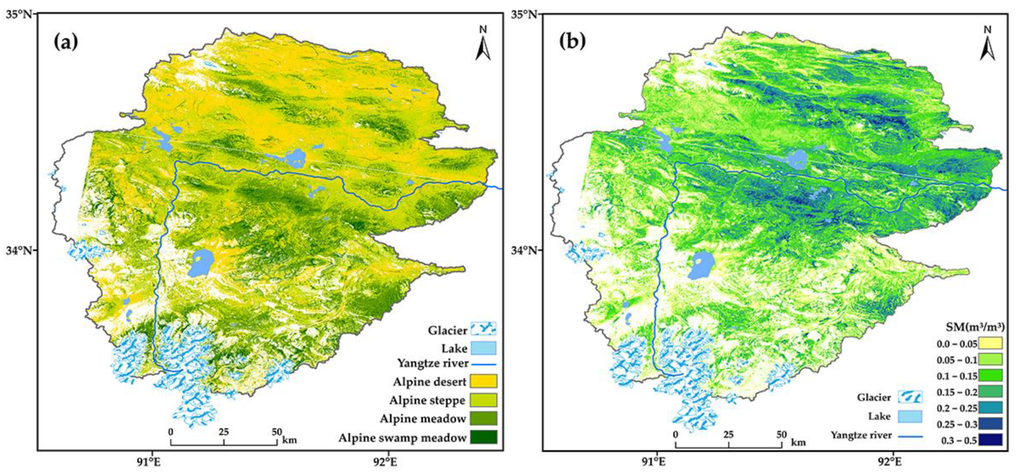
3.3. Map of Retrieved SM

Figure 8 shows retrieved SM on eight days of S1 acquisitions with the grid spacing of 50 m × 50 m. The white areas in the retrieval results are caused by post-processing, where water bodies, mountain shadows, and anomalous areas are masked. To better show the spatial distribution characteristics of SM, Figure 9 was made by overlaying the spatial distribution map of SM with the topographic map. In hill areas with undulating terrain, SM is usually higher. In order to show the complexity of the spatial distribution of SM in mountainous areas of the permafrost region, this study designed two transect lines to further show the SM variation in the hill areas and extracted the SM values corresponding to the two transect lines, as shown in Figure 10. The variability of SM in hill areas is well presented. It demonstrates the high variability of SM, which could not be revealed by coarse SM products.
Figure 11 shows the relationship between the spatial and temporal CV and the mean SM in this study area. The CV tends to decrease with increasing mean SM in both spatial and temporal dimensions, which shows that the variability of SM is higher in drier environments and lower in wetter environments. This pattern is related to the water-holding capacity of the soil and its spatial variability [83]. The large differences in the CV in different regions are related to the soil water content, bulk density, and soil texture [22,84,85]. In permafrost areas, the physicochemical properties of soils vary greatly in different areas of topography and vegetation cover, resulting in a high spatial heterogeneity of SM. In addition, the high CV in areas of low SM may also be explained by frequent precipitation and strong evapotranspiration during the thawing season.

4. Discussion

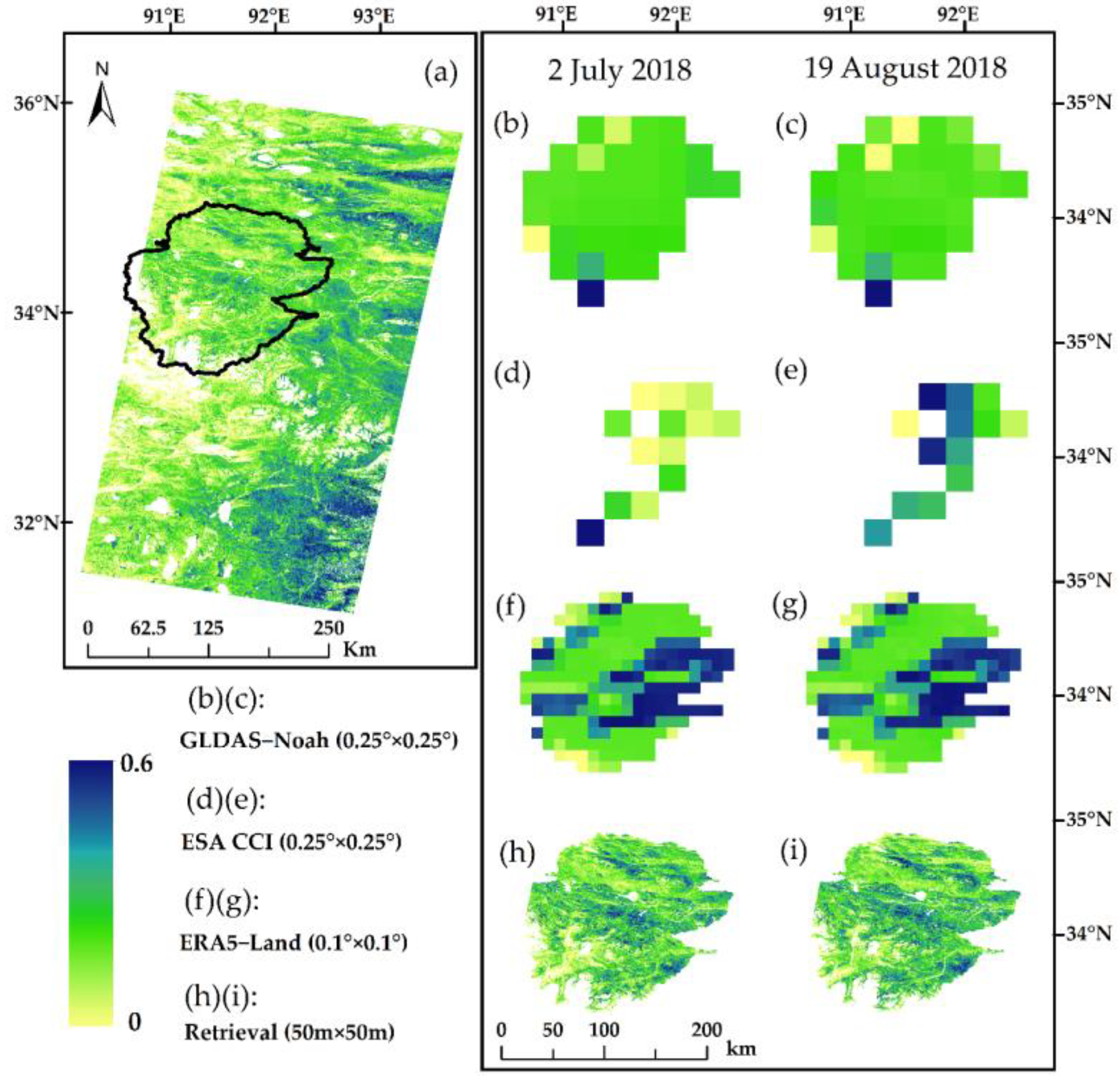
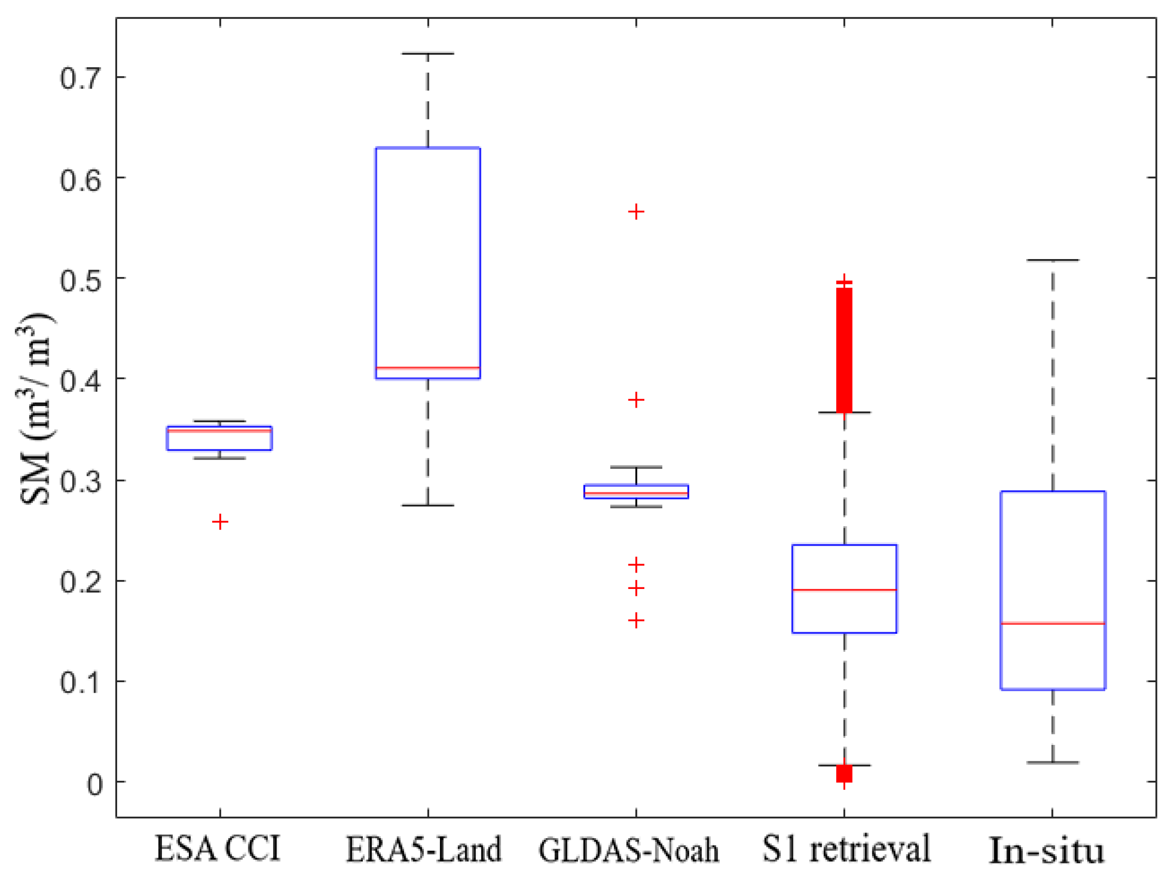
4.1. Comparison of S1-Retrieved SM with SM Products

We chose the Tuotuo River basin as an example, where the detailed investigation was conducted, to compare with widely used SM products, such as GLDAS-Noah, ESA CCI, and ERA5-Land (Figure 12). At the local scale, the retrieval results can present the distribution characteristics of SM in different surface environments. The widely used SM data products are unable to characterize the heterogeneity of SM spatial distribution in detail. For example, the GLDAS and CCI can only identify high SM in the southernmost glacial regions, while the distribution of SM in other areas is varied. They can only give a very rough description of the moisture distribution over tens of kilometers limited by its coarse resolution, and the details on SM distribution are lost. In addition, the distribution of the three SM products in this region is also different, which also confirms the demand for high-accuracy SM data in the QTP.
Figure 13 shows the statistics of SM distribution in the study area on 2 July 2018, from three SM products and S1 retrieval results. The average SM content of ESA CCI, ERA5-Land, GLDAS-Noah, and retrieval result is 0.34, 0.5, 0.29, and 0.19, respectively. The upper and lower quartiles of the in situ SM for the thawing season are 0.29 and 0.09, respectively. Compared with the in situ data, the SM values of the three products are significantly overestimated, while the retrieval results are in a reasonable range. In addition, previous research found that the SM data of the ESA CCI product has the best accuracy on the QTP compared with in situ observations, with an r of 0.63 [16]. In terms of accuracy, our SM retrieval results also showed substantially higher accuracy, and r reached 0.9.

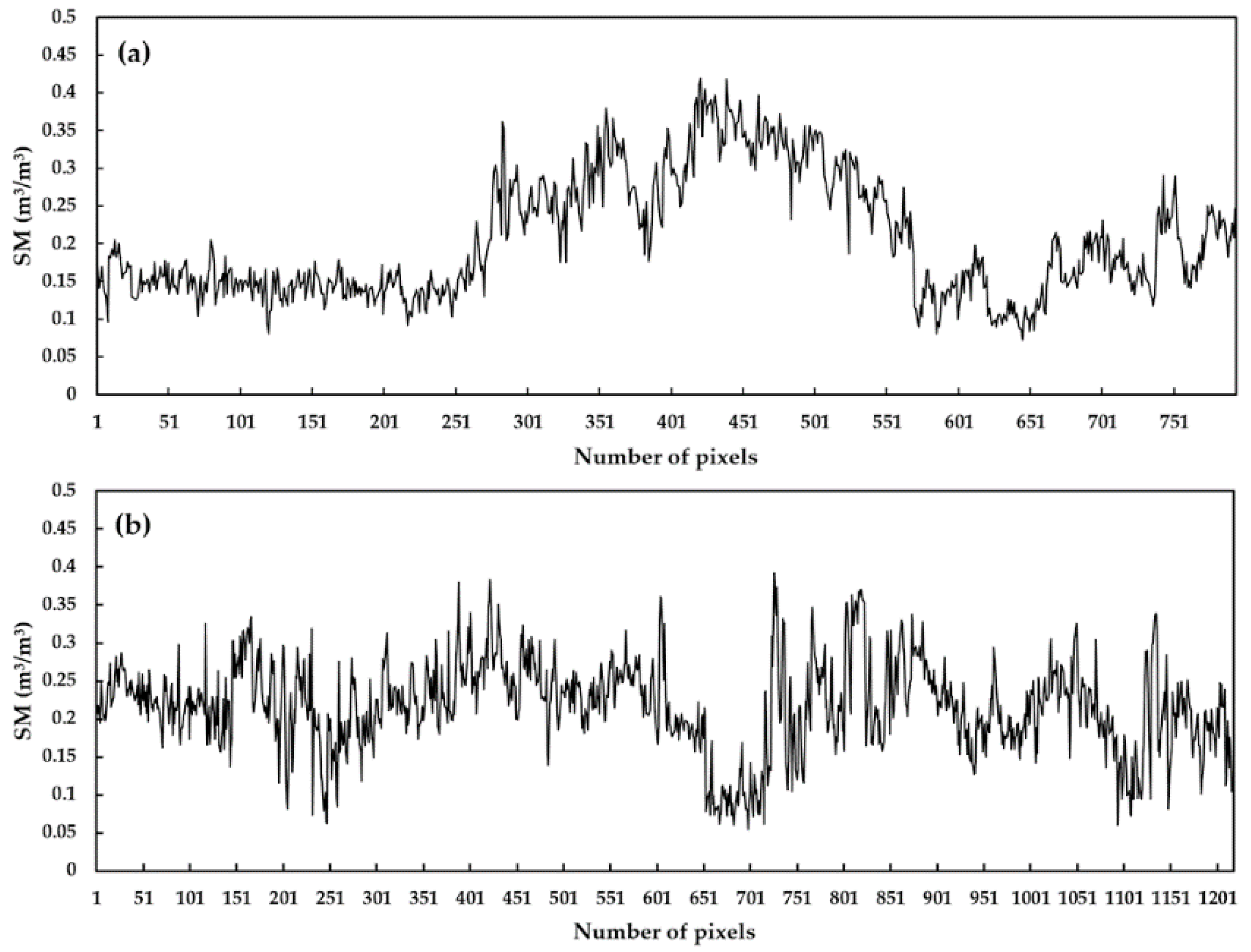
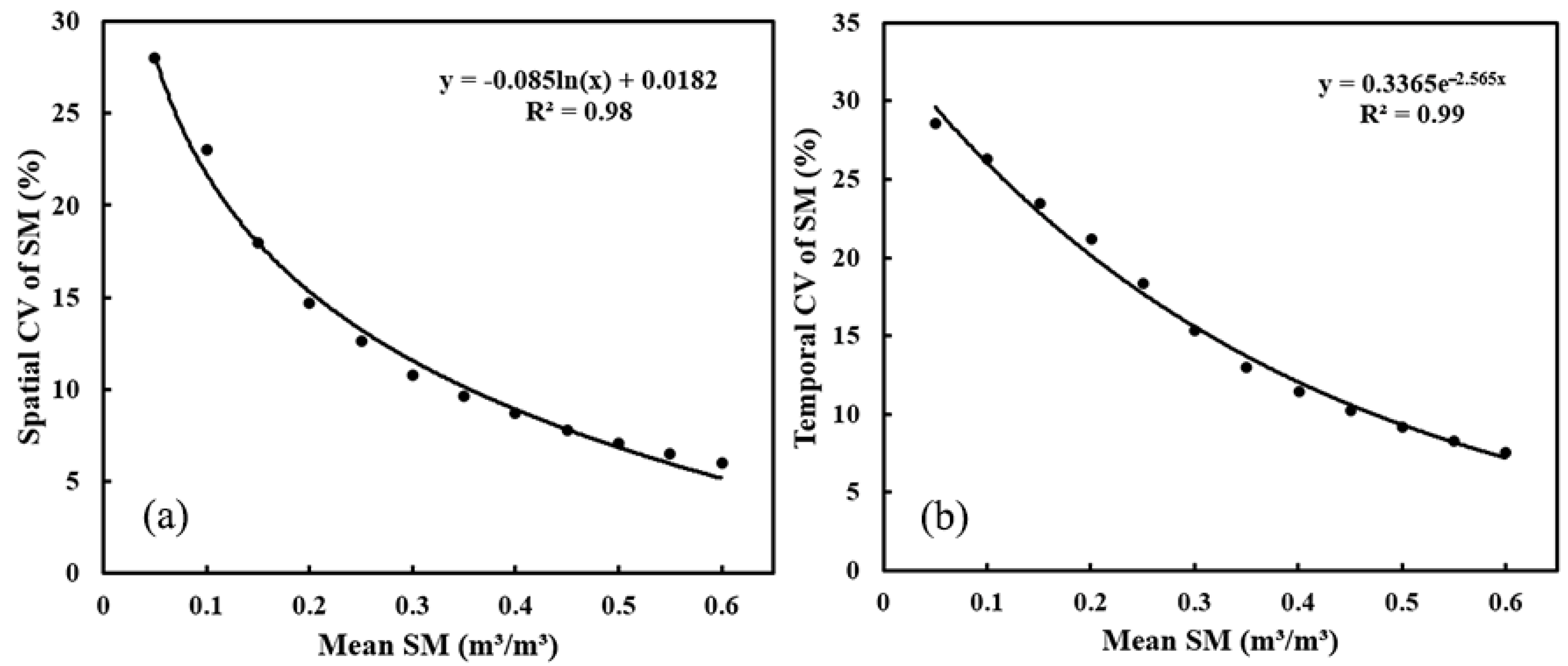
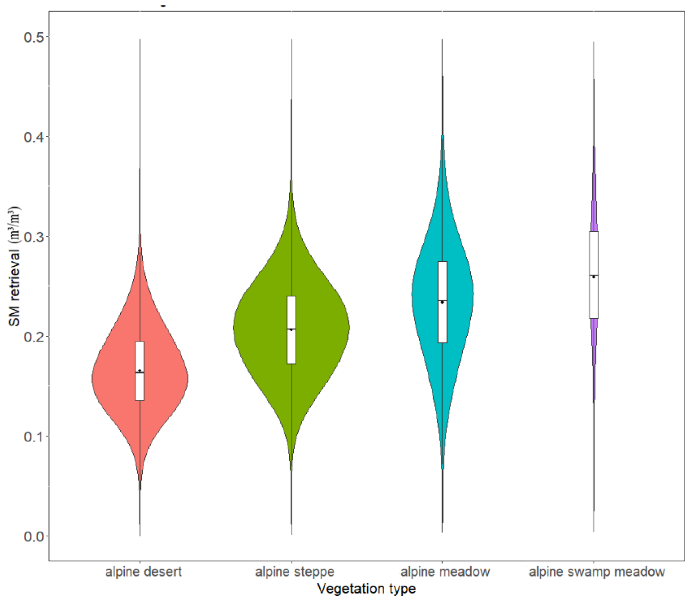
4.2. SM Distribution Characteristics at the Local Scale

Figure 14 shows the spatial distribution of different vegetation types [86] and SM in the Tuotuo River basin. We summarized the characteristics of SM over different vegetation types, as shown in Figure 15. In areas with high vegetation cover, such as alpine swamp meadows and alpine meadow areas, the SM content is significantly higher than in alpine steppe and alpine desert areas. The average SM content over different vegetation types from high to low is alpine swamp meadow (0.26), alpine meadow (0.23), alpine steppe (0.20), and alpine desert (0.16).

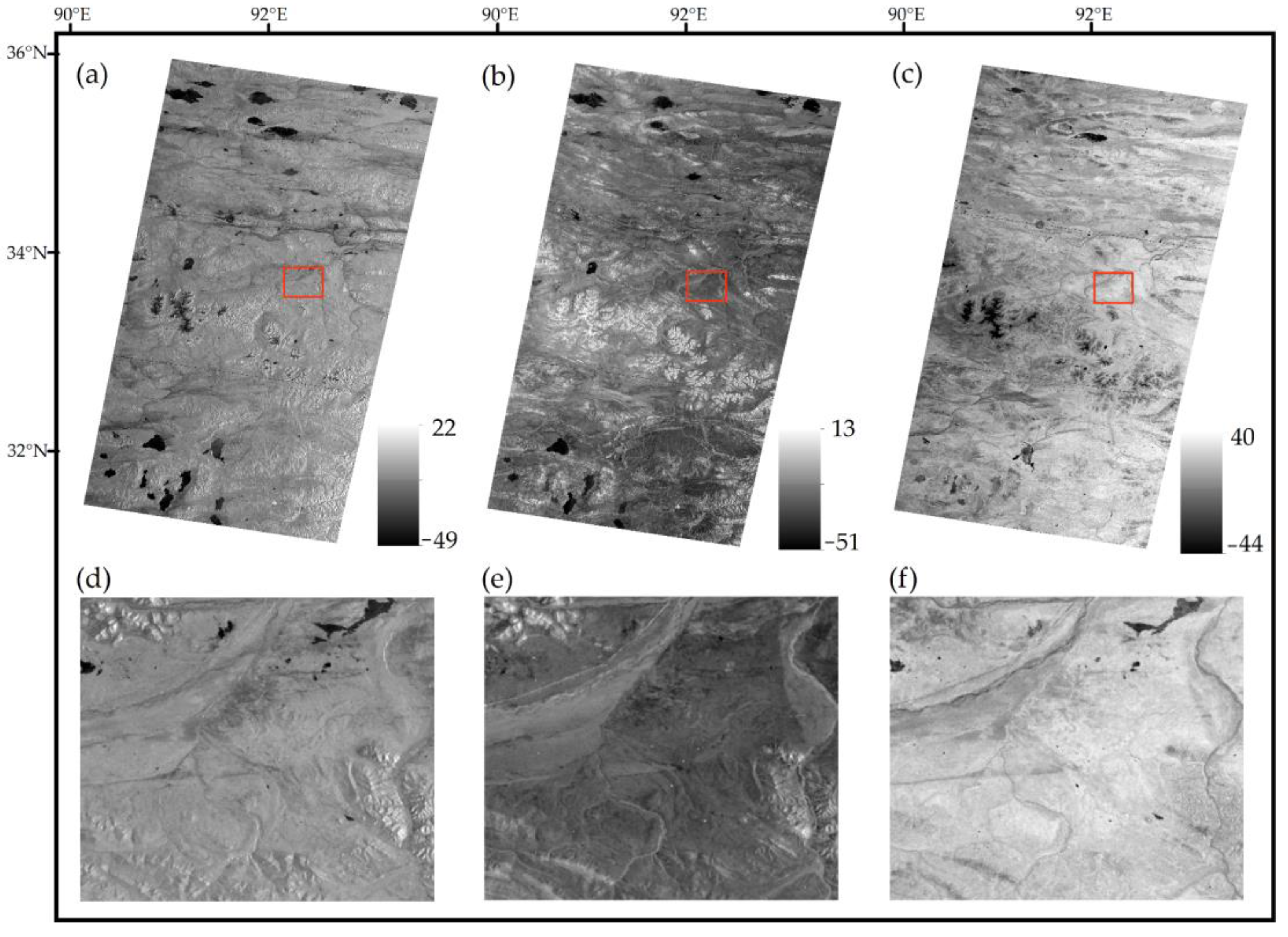
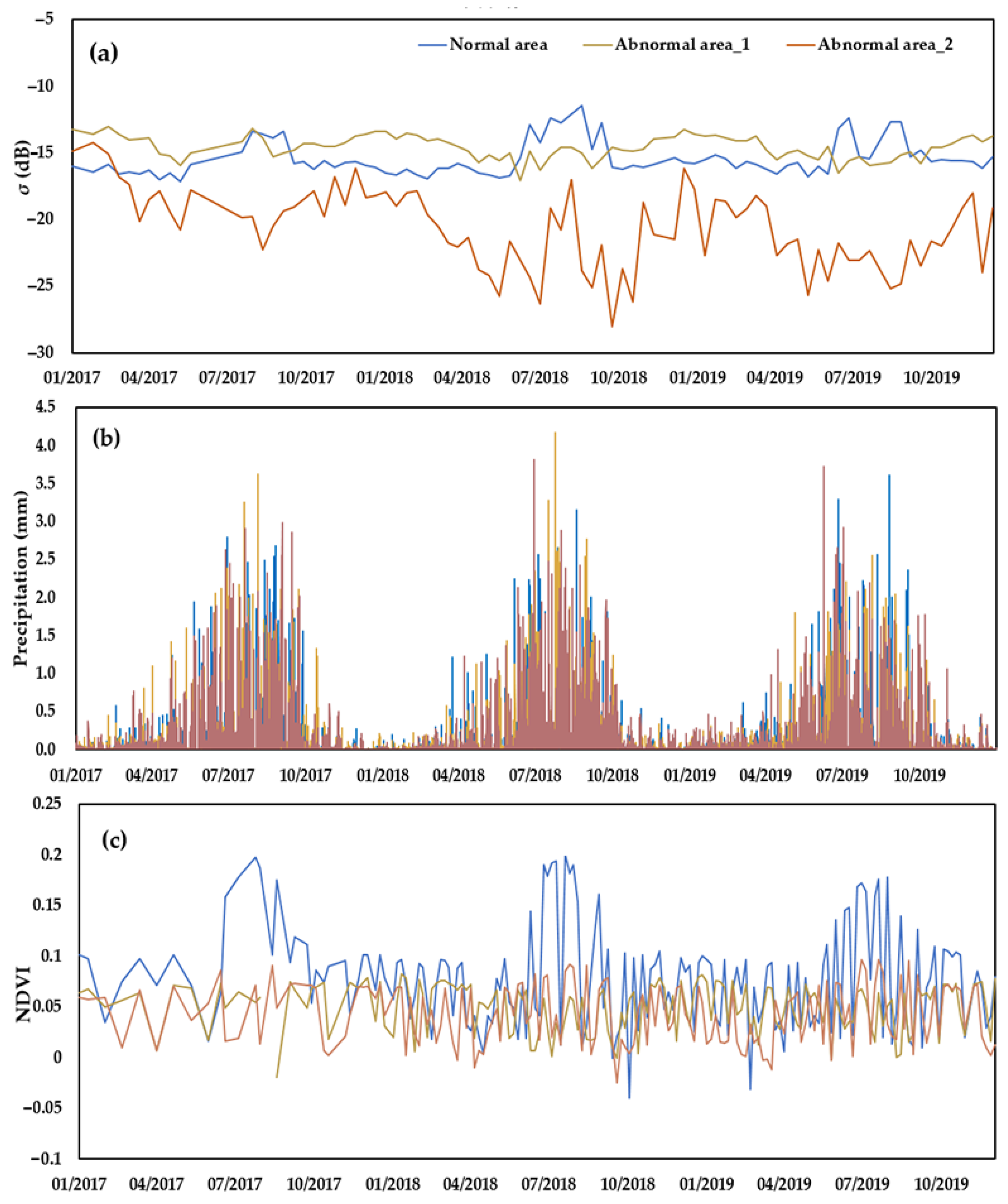
4.3. Regions with Very Low σ° in the Thawing Season

Normally, the value of σ° in the thawing season is higher than that in winter because the liquid water content in the thawing state is usually higher than in the frozen state [87]. However, during the SM retrieving process, we noticed that σ° during the thawing season in some regions is close to or even lower than σ° in winter. Therefore, we tried to find the reason by comparing the variation of the backscattering coefficients for long time series. As shown in Figure 16a, we consider the regions with significant seasonal variations in the σ° as normal areas, i.e., σ° is higher in summer than in winter, and the disordered areas as abnormal areas. To explain the potential reasons for this phenomenon, we further examined the precipitation, vegetation, and soil texture in these particular regions.
  • Precipitation
The precipitation process during the thawing season is one of the main reasons for SM variations [88]. During precipitation events, the wet or flooded ground surface will cause the σ° to deviate from its normal range. We examined the precipitation conditions in three regions as in Figure 16a to test the possibility of this conjecture. The precipitation data is from ERA5-Land precipitation reanalysis data [13], and the temporal curves are shown in Figure 16b. The average annual precipitation of the three regions is 606 mm, 574 mm, and 624 mm, respectively, with little difference in precipitation. Therefore, precipitation is not the cause of low σ° in the thawing season, and the speculation that the wet ground surface causes low σ° is not true. The inference of the abnormal σ° caused by the accumulation of surface water is also not valid.
  • Vegetation and soil texture
The impact of vegetation coverage and soil texture on SM content should not be neglected [89,90,91]. We found some differences between the two regions by examining the temporal changes in the NDVI values in the normal and abnormal regions. As shown in Figure 16c, the NDVI values in the abnormal areas are all relatively low (smaller than 0.1) and do not exhibit seasonal variations. Meanwhile, we referred to the soil texture dataset published by Liu et al. [92,93] and combined it with the field records in the anomaly areas. We found that the soil in this abnormal area is composed of sand. There is a big chance that these abnormal areas are bare ground and are extremely dry during the particular period in the thawing season, therefore leading to low values of σ°.

5. Conclusions

This study developed a concise and practical algorithm for SM estimation using Sentinel-1/2 temporal data in a permafrost environment on the QTP in the thawing season. The R2 of this SM retrieval algorithm reached 0.82 with an RMSE of 0.06 m3/m3.
Our retrieved SM results were compared with current SM products (ERA5-Land, GLDAS-Noah, and ESA CCI) in the Tuotuo River basin and showed that our results have more strength and advantage in characterizing the spatial heterogeneity of SM distribution. By analyzing the SM distribution of different vegetation types, the alpine swamp meadow had the largest SM of 0.26 m3/m3, followed by the alpine meadow (0.23), alpine steppe (0.2), and alpine desert (0.16). We also found a significantly negative correlation between the CV and SM in the permafrost area that the variability of SM is higher in drier environments and lower in wetter environments.
The study also explored the reasons for abnormal SM retrievals in some places. The developed algorithm is not applicable in some extremely bare and dry ground with very low SM. Overall, the proposed algorithm shows great potential to derive the detailed SM distribution in the permafrost environment on the entire QTP, which has great significance in studying the SM characteristics in spatial detail and helps facilitate the studies of the response of permafrost to climate change.

Author Contributions

Z.L., L.Z. and L.W. conceived and designed the experiments; Z.L., L.W., D.Z., E.D., Y.X., Z.X., S.L., H.Z. and Y.C. performed the experiments; and Z.L., L.Z., L.W., G.L., G.H., J.Z., C.W., Y.Q. and J.S. analyzed the data and wrote the paper. All of the authors contributed to the editing of the manuscript. All authors have read and agreed to the published version of the manuscript.

Funding

This research was funded by the Second Tibetan Plateau Scientific Expedition and Research Program (2019QZKK0201), the National Natural Science Foundation of China (41931180, 42001054, 42001051), and the Youth Fund for Basic Research Program of Jiangsu Province (BK20200828).

Acknowledgments

We are grateful to the anonymous reviewers and editors for appraising our manuscript and offering instructive comments. We are very grateful to Lei Fan and Xiaojing Bai for their guidance on the experiments of this paper. We also appreciate the free access to data sets from the Chinese Academy of Sciences. In addition, we would like to thank the Google Earth Engine platform for providing the data and processing methods needed in this study.

Conflicts of Interest

The authors declare no conflict of interest.

References

  1. Jin, R.; Li, X.; Liu, S. Understanding the heterogeneity of soil moisture and evapotranspiration using multiscale observations from satellites, airborne sensors, and a ground-based observation matrix. IEEE Geosci. Remote Sens. Lett. 2017, 14, 2132–2136. [Google Scholar] [CrossRef]
  2. Seneviratne, S.I.; Corti, T.; Davin, E.L.; Hirschi, M.; Jaeger, E.B.; Lehner, I.; Orlowsky, B.; Teuling, A.J. Investigating soil moisture–climate interactions in a changing climate: A review. Earth Sci. Rev. 2010, 99, 125–161. [Google Scholar] [CrossRef]
  3. Assouline, S. Infiltration into soils: Conceptual approaches and solutions. Water Resour. Res. 2013, 49, 1755–1772. [Google Scholar] [CrossRef]
  4. Crowther, T.W.; Todd-Brown, K.E.; Rowe, C.W.; Wieder, W.R.; Carey, J.C.; Machmuller, M.B.; Snoek, B.; Fang, S.; Zhou, G.; Allison, S.D. Quantifying global soil carbon losses in response to warming. Nature 2016, 540, 104–108. [Google Scholar] [CrossRef] [PubMed] [Green Version]
  5. Moghaddam, M.A.; Ferre, T.; Chen, X.; Chen, K.; Ehsani, M.R. Application of Machine Learning Methods in Inferring Surface Water Groundwater Exchanges using High Temporal Resolution Temperature Measurements. arXiv 2022, arXiv:2201.00726. [Google Scholar]
  6. Zeng, J.; Li, Z.; Chen, Q.; Bi, H.; Qiu, J.; Zou, P. Evaluation of remotely sensed and reanalysis soil moisture products over the Tibetan Plateau using in-situ observations. Remote Sens. Environ. 2015, 163, 91–110. [Google Scholar] [CrossRef]
  7. Yi, S.; Wang, X.; Qin, Y.; Xiang, B.; Ding, Y. Responses of alpine grassland on Qinghai–Tibetan plateau to climate warming and permafrost degradation: A modeling perspective. Environ. Res. Lett. 2014, 9, 074014. [Google Scholar] [CrossRef] [Green Version]
  8. Zhao, L.; Cheng, G.; Li, S.; Zhao, X.; Wang, S. Thawing and freezing processes of active layer in Wudaoliang region of Tibetan Plateau. Chin. Sci. Bull. 2000, 45, 2181–2187. [Google Scholar] [CrossRef]
  9. Xu, L.; Abbaszadeh, P.; Moradkhani, H.; Chen, N.; Zhang, X. Continental drought monitoring using satellite soil moisture, data assimilation and an integrated drought index. Remote Sens. Environ. 2020, 250, 112028. [Google Scholar] [CrossRef]
  10. Zou, D.; Zhao, L.; Sheng, Y.; Chen, J.; Hu, G.; Wu, T.; Wu, J.; Xie, C.; Wu, X.; Pang, Q. A new map of permafrost distribution on the Tibetan Plateau. Cryosphere 2017, 11, 2527–2542. [Google Scholar] [CrossRef] [Green Version]
  11. Zhao, L.; Zou, D.; Hu, G.; Wu, T.; Du, E.; Liu, G.; Xiao, Y.; Li, R.; Pang, Q.; Qiao, Y. A synthesis dataset of permafrost thermal state for the Qinghai–Tibet (Xizang) Plateau, China. Earth Syst. Sci. Data 2021, 13, 4207–4218. [Google Scholar] [CrossRef]
  12. Zhuang, R.; Zeng, Y.; Manfreda, S.; Su, Z. Quantifying Long-Term Land Surface and Root Zone Soil Moisture over Tibetan Plateau. Remote Sens. 2020, 12, 509. [Google Scholar] [CrossRef] [Green Version]
  13. Muñoz-Sabater, J.; Dutra, E.; Balsamo, G.; Boussetta, S.; Zsoter, E.; Albergel, C.; Agusti-Panareda, A. ERA5-Land: An improved version of the ERA5 reanalysis land component. In Proceedings of the 8th Workshop-Joint ISWG and LSA-SAF Workshop, Lisbon, Portugal, 26–28 June 2018; pp. 26–28. [Google Scholar]
  14. Dorigo, W.; Wagner, W.; Albergel, C.; Albrecht, F.; Balsamo, G.; Brocca, L.; Chung, D.; Ertl, M.; Forkel, M.; Gruber, A. ESA CCI Soil Moisture for improved Earth system understanding: State-of-the art and future directions. Remote Sens. Environ. 2017, 203, 185–215. [Google Scholar] [CrossRef]
  15. Rodell, M.; Houser, P.; Jambor, U.; Gottschalck, J.; Mitchell, K.; Meng, C.-J.; Arsenault, K.; Cosgrove, B.; Radakovich, J.; Bosilovich, M. The global land data assimilation system. Bull. Am. Meteorol. Soc. 2004, 85, 381–394. [Google Scholar] [CrossRef] [Green Version]
  16. Xing, Z.; Fan, L.; Zhao, L.; De Lannoy, G.; Frappart, F.; Peng, J.; Li, X.; Zeng, J.; Al-Yaari, A.; Yang, K. A first assessment of satellite and reanalysis estimates of surface and root-zone soil moisture over the permafrost region of Qinghai-Tibet Plateau. Remote Sens. Environ. 2021, 265, 112666. [Google Scholar] [CrossRef]
  17. Liu, J.; Chai, L.; Lu, Z.; Liu, S.; Qu, Y.; Geng, D.; Song, Y.; Guan, Y.; Guo, Z.; Wang, J. Evaluation of SMAP, SMOS-IC, FY3B, JAXA, and LPRM Soil moisture products over the Qinghai-Tibet Plateau and Its surrounding areas. Remote Sens. 2019, 11, 792. [Google Scholar] [CrossRef] [Green Version]
  18. Ivanov, V.Y.; Fatichi, S.; Jenerette, G.D.; Espeleta, J.F.; Troch, P.A.; Huxman, T.E. Hysteresis of soil moisture spatial heterogeneity and the “homogenizing” effect of vegetation. Water Resour. Res. 2010, 46, W09521. [Google Scholar] [CrossRef]
  19. Srivastava, A.; Saco, P.M.; Rodriguez, J.F.; Kumari, N.; Chun, K.P.; Yetemen, O. The role of landscape morphology on soil moisture variability in semi-arid ecosystems. Hydrol. Process. 2021, 35, e13990. [Google Scholar] [CrossRef]
  20. Fatichi, S.; Katul, G.G.; Ivanov, V.Y.; Pappas, C.; Paschalis, A.; Consolo, A.; Kim, J.; Burlando, P. Abiotic and biotic controls of soil moisture spatiotemporal variability and the occurrence of hysteresis. Water Resour. Res. 2015, 51, 3505–3524. [Google Scholar] [CrossRef]
  21. Baroni, G.; Ortuani, B.; Facchi, A.; Gandolfi, C. The role of vegetation and soil properties on the spatio-temporal variability of the surface soil moisture in a maize-cropped field. J. Hydrol. 2013, 489, 148–159. [Google Scholar] [CrossRef]
  22. Rosenbaum, U.; Bogena, H.R.; Herbst, M.; Huisman, J.A.; Peterson, T.J.; Weuthen, A.; Western, A.W.; Vereecken, H. Seasonal and event dynamics of spatial soil moisture patterns at the small catchment scale. Water Resour. Res. 2012, 48, W10544. [Google Scholar] [CrossRef]
  23. Tomer, S.K.; Al Bitar, A.; Sekhar, M.; Zribi, M.; Bandyopadhyay, S.; Kerr, Y. MAPSM: A spatio-temporal algorithm for merging soil moisture from active and passive microwave remote sensing. Remote Sens. 2016, 8, 990. [Google Scholar] [CrossRef] [Green Version]
  24. Torres, R.; Snoeij, P.; Geudtner, D.; Bibby, D.; Davidson, M.; Attema, E.; Potin, P.; Rommen, B.; Floury, N.; Brown, M. GMES Sentinel-1 mission. Remote Sens. Environ. 2012, 120, 9–24. [Google Scholar] [CrossRef]
  25. Baghdadi, N.; Pedreros, R.; Lenotre, N.; Dewez, T.; Paganini, M. Impact of polarization and incidence of the ASAR sensor on coastline mapping: Example of Gabon. Int. J. Remote Sens. 2007, 28, 3841–3849. [Google Scholar] [CrossRef]
  26. Zribi, M.; Baghdadi, N.; Holah, N.; Fafin, O. New methodology for soil surface moisture estimation and its application to ENVISAT-ASAR multi-incidence data inversion. Remote Sens. Environ. 2005, 96, 485–496. [Google Scholar] [CrossRef]
  27. Ulaby, F.T.; Sarabandi, K.; Mcdonald, K.; Whitt, M.; Dobson, M.C. Michigan microwave canopy scattering model. Int. J. Remote Sens. 1990, 11, 1223–1253. [Google Scholar] [CrossRef]
  28. Chen, K.; Yen, S.; Huang, W. A simple model for retrieving bare soil moisture from radar-scattering coefficients. Remote Sens. Environ. 1995, 54, 121–126. [Google Scholar] [CrossRef]
  29. Dubois, P.C.; Van Zyl, J.; Engman, T. Measuring soil moisture with imaging radars. IEEE Trans. Geosci. Remote Sens. 1995, 33, 915–926. [Google Scholar] [CrossRef] [Green Version]
  30. Oh, Y.; Sarabandi, K.; Ulaby, F.T. Semi-empirical model of the ensemble-averaged differential Mueller matrix for microwave backscattering from bare soil surfaces. IEEE Trans. Geosci. Remote Sens. 2002, 40, 1348–1355. [Google Scholar] [CrossRef] [Green Version]
  31. Fung, A.K.; Shah, M.R.; Tjuatja, S. Numerical simulation of scattering from three-dimensional randomly rough surfaces. IEEE Trans. Geosci. Remote Sens. 1994, 32, 986–994. [Google Scholar] [CrossRef]
  32. Attema, E.; Ulaby, F.T. Vegetation modeled as a water cloud. Radio Sci. 1978, 13, 357–364. [Google Scholar] [CrossRef]
  33. Allen, C.; Ulaby, F. Modelling the polarization dependence of the attenuation in vegetation canopies. In Proceedings of the IGARSS, Strasbourg, France, 27–30 August 1984; pp. 119–124. [Google Scholar]
  34. He, B.; Xing, M.; Bai, X. A Synergistic Methodology for Soil Moisture Estimation in an Alpine Prairie Using Radar and Optical Satellite Data. Remote Sens. 2014, 6, 10966–10985. [Google Scholar] [CrossRef] [Green Version]
  35. Bai, X.; He, B.; Li, X.; Zeng, J.; Wang, X.; Wang, Z.; Zeng, Y.; Su, Z. First Assessment of Sentinel-1A Data for Surface Soil Moisture Estimations Using a Coupled Water Cloud Model and Advanced Integral Equation Model over the Tibetan Plateau. Remote Sens. 2017, 9, 714. [Google Scholar] [CrossRef] [Green Version]
  36. Yang, M.; Wang, H.; Tong, C.; Zhu, L.; Deng, X.; Deng, J.; Wang, K. Soil moisture retrievals using multi-temporal sentinel-1 data over nagqu region of tibetan plateau. Remote Sens. 2021, 13, 1913. [Google Scholar] [CrossRef]
  37. Kornelsen, K.C.; Coulibaly, P. Advances in soil moisture retrieval from synthetic aperture radar and hydrological applications. J. Hydrol. 2013, 476, 460–489. [Google Scholar] [CrossRef]
  38. Zhu, L.; Walker, J.P.; Tsang, L.; Huang, H.; Ye, N.; Rüdiger, C. A multi-frequency framework for soil moisture retrieval from time series radar data. Remote Sens. Environ. 2019, 235, 111433. [Google Scholar] [CrossRef]
  39. Wagner, W.; Lemoine, G.; Rott, H. A method for estimating soil moisture from ERS scatterometer and soil data. Remote Sens. Environ. 1999, 70, 191–207. [Google Scholar] [CrossRef]
  40. Gao, Q.; Zribi, M.; Escorihuela, M.J.; Baghdadi, N. Synergetic use of Sentinel-1 and Sentinel-2 data for soil moisture mapping at 100 m resolution. Sensors 2017, 17, 1966. [Google Scholar] [CrossRef] [Green Version]
  41. Paloscia, S.; Pettinato, S.; Santi, E.; Notarnicola, C.; Pasolli, L.; Reppucci, A. Soil moisture mapping using Sentinel-1 images: Algorithm and preliminary validation. Remote Sens. Environ. 2013, 134, 234–248. [Google Scholar] [CrossRef]
  42. Bauer-Marschallinger, B.; Freeman, V.; Cao, S.; Paulik, C.; Schaufler, S.; Stachl, T.; Modanesi, S.; Massari, C.; Ciabatta, L.; Brocca, L.; et al. Toward Global Soil Moisture Monitoring With Sentinel-1: Harnessing Assets and Overcoming Obstacles. IEEE Trans. Geosci. Remote Sens. 2019, 57, 520–539. [Google Scholar] [CrossRef]
  43. Zhu, L.; Si, R.; Shen, X.; Walker, J.P. An advanced change detection method for time-series soil moisture retrieval from Sentinel-1. Remote Sens. Environ. 2022, 279, 113137. [Google Scholar] [CrossRef]
  44. Zhu, L.; Walker, J.P.; Ye, N.; Rüdiger, C. Roughness and vegetation change detection: A pre-processing for soil moisture retrieval from multi-temporal SAR imagery. Remote Sens. Environ. 2019, 225, 93–106. [Google Scholar] [CrossRef]
  45. Zhang, X.; Zhang, H.; Wang, C.; Tang, Y.; Zhang, B.; Wu, F.; Wang, J.; Zhang, Z. Soil Moisture Estimation based on the Distributed Scatterers Adaptive Filter over the QTP Permafrost Region using Sentinel-1 and High-resolution TerraSAR-X Data. Int. J. Remote Sens. 2021, 42, 902–928. [Google Scholar] [CrossRef]
  46. Li, Y.; Guan, D.; Zhao, L.; Gu, S.; Zhao, X. Seasonal frozen soil and its effect on vegetation production in Haibei alpine meadow. J. Glaciol. Geocryol. 2005, 27, 311–319. [Google Scholar]
  47. Li, H.; Liu, F.; Zhang, S.; Zhang, C.; Zhang, C.; Ma, W.; Luo, J. Drying–Wetting Changes of Surface Soil Moisture and the Influencing Factors in Permafrost Regions of the Qinghai-Tibet Plateau, China. Remote Sens. 2022, 14, 2915. [Google Scholar] [CrossRef]
  48. Bindlish, R.; Barros, A.P. Parameterization of vegetation backscatter in radar-based, soil moisture estimation. Remote Sens. Environ. 2001, 76, 130–137. [Google Scholar] [CrossRef]
  49. Baghdadi, N.; El Hajj, M.; Zribi, M.; Bousbih, S. Calibration of the water cloud model at C-band for winter crop fields and grasslands. Remote Sens. 2017, 9, 969. [Google Scholar] [CrossRef] [Green Version]
  50. Zeng, X.; Xing, Y.; Shan, W.; Zhang, Y.; Wang, C. Soil water content retrieval based on Sentinel-1A and Landsat 8 image for Bei’an-Heihe Expressway. Zhongguo Shengtai Nongye Xuebao/Chin. J. Eco-Agric. 2017, 25, 118–126. [Google Scholar]
  51. Hajj, M.E.; Bégué, A.; Lafrance, B.; Hagolle, O.; Dedieu, G.; Rumeau, M. Relative radiometric normalization and atmospheric correction of a SPOT 5 time series. Sensors 2008, 8, 2774–2791. [Google Scholar] [CrossRef] [Green Version]
  52. Kumari, N.; Srivastava, A.; Dumka, U.C. A long-term spatiotemporal analysis of vegetation greenness over the himalayan region using google earth engine. Climate 2021, 9, 109. [Google Scholar] [CrossRef]
  53. El Hajj, M.; Baghdadi, N.; Zribi, M.; Belaud, G.; Cheviron, B.; Courault, D.; Charron, F. Soil moisture retrieval over irrigated grassland using X-band SAR data. Remote Sens. Environ. 2016, 176, 202–218. [Google Scholar] [CrossRef] [Green Version]
  54. Bao, Y.; Lin, L.; Wu, S.; Deng, K.A.K.; Petropoulos, G.P. Surface soil moisture retrievals over partially vegetated areas from the synergy of Sentinel-1 and Landsat 8 data using a modified water-cloud model. Int. J. Appl. Earth Obs. Geoinf. 2018, 72, 76–85. [Google Scholar] [CrossRef]
  55. Wigneron, J.P.; Kerr, Y.; Waldteufel, P.; Saleh, K.; Escorihuela, M.J.; Richaume, P.; Ferrazzoli, P.; Rosnay, P.D.; Gurney, R.; Calvet, J.C. L-band Microwave Emission of the Biosphere (L-MEB) Model: Description and calibration against experimental data sets over crop fields. Remote Sens. Environ. 2007, 107, 639–655. [Google Scholar] [CrossRef]
  56. Zhao, L.; Zou, D.; Hu, G.; Du, E.; Pang, Q.; Xiao, Y.; Li, R.; Sheng, Y.; Wu, X.; Sun, Z. Changing climate and the permafrost environment on the Qinghai–Tibet (Xizang) plateau. Permafr. Periglac. Process. 2020, 31, 396–405. [Google Scholar] [CrossRef]
  57. Lin, Z.; Guojie, H.; Defu, Z.; Xiaodong, W.; Lu, M.; Zhe, S.; Liming, Y.; Huayun, Z.; Shibo, L. Permafrost changes and its effects on hydrological processes on Qinghai-Tibet Plateau. Bull. Chin. Acad. Sci. 2019, 34, 1233–1246. [Google Scholar]
  58. Cheng, G.; Zhao, L.; Li, R.; Wu, X.; Sheng, Y.; Hu, G.; Zou, D.; Jin, H.; Li, X.; Wu, Q. Characteristic, changes and impacts of permafrost on Qinghai-Tibet Plateau. Chin. Sci. Bull. 2019, 64, 2783–2795. [Google Scholar]
  59. Wang, Z.W.; Wang, Q.; Zhao, L.; Wu, X.D.; Yue, G.Y.; Zou, D.F.; Nan, Z.T.; Liu, G.Y.; Pang, Q.Q.; Fang, H.B.; et al. Mapping the vegetation distribution of the permafrost zone on the Qinghai-Tibet Plateau. J. Mt. Sci. 2016, 13, 1035–1046. [Google Scholar] [CrossRef]
  60. Lin, Z.; Burn, C.R.; Niu, F.; Luo, J.; Liu, M.; Yin, G. The thermal regime, including a reversed thermal offset, of arid permafrost sites with variations in vegetation cover density, Wudaoliang Basin, Qinghai-Tibet plateau. Permafr. Periglac. Process. 2015, 26, 142–159. [Google Scholar] [CrossRef]
  61. Li, R.; Zhao, L.; Ding, Y.; Wu, T.; Xiao, Y.; Du, E.; Liu, G.; Qiao, Y. Temporal and spatial variations of the active layer along the Qinghai-Tibet Highway in a permafrost region. Chin. Sci. Bull. 2012, 57, 4609–4616. [Google Scholar] [CrossRef] [Green Version]
  62. Shiyin, L.; Wanqin, G.; Junli, X. The Second Glacier Inventory Dataset of China (Version 1.0) (2006–2011); National Tibetan Plateau Data Center: Beijing, China, 2012. [Google Scholar]
  63. Messager, M.L.; Lehner, B.; Grill, G.; Nedeva, I.; Schmitt, O. Estimating the volume and age of water stored in global lakes using a geo-statistical approach. Nat. Commun. 2016, 7, 13603. [Google Scholar] [CrossRef]
  64. Farr, T.G.; Rosen, P.A.; Ro, E.C.; Crippen, R.; Duren, R.; Hensley, S.; Kobrick, M.; Paller, M.; Rodriguez, E.; Roth, L. The Shuttle Radar Topography Mission. Rev. Geophys. 2007, 45, 361. [Google Scholar] [CrossRef] [Green Version]
  65. Bai, X.; He, B. Potential of Dubois model for soil moisture retrieval in prairie areas using SAR and optical data. Int. J. Remote Sens. 2015, 36, 5737–5753. [Google Scholar] [CrossRef]
  66. Amazirh, A.; Merlin, O.; Er-Raki, S.; Gao, Q.; Rivalland, V.; Malbeteau, Y.; Khabba, S.; Escorihuela, M. Retrieving surface soil moisture at high spatio-temporal resolution from a synergy between Sentinel-1 radar and Landsat thermal data: A study case over bare soil. Remote Sens. Environ. 2018, 211, 321–337. [Google Scholar] [CrossRef]
  67. Bousbih, S.; Zribi, M.; Lili-Chabaane, Z.; Baghdadi, N.; Mougenot, B. Potential of Sentinel-1 Radar Data for the Assessment of Soil and Cereal Cover Parameters. Sensors 2017, 17, 2617. [Google Scholar] [CrossRef] [Green Version]
  68. Dabrowska-Zielinska, K.; Musial, J.; Malinska, A.; Budzynska, M.; Gurdak, R.; Kiryla, W.; Bartold, M.; Grzybowski, P. Soil moisture in the Biebrza Wetlands retrieved from Sentinel-1 imagery. Remote Sens. 2018, 10, 1979. [Google Scholar] [CrossRef]
  69. Li, J.; Roy, D.P. A global analysis of Sentinel-2A, Sentinel-2B and Landsat-8 data revisit intervals and implications for terrestrial monitoring. Remote Sens. 2017, 9, 902. [Google Scholar] [CrossRef] [Green Version]
  70. Drusch, M.; Del Bello, U.; Carlier, S.; Colin, O.; Fernandez, V.; Gascon, F.; Hoersch, B.; Isola, C.; Laberinti, P.; Martimort, P. Sentinel-2: ESA’s optical high-resolution mission for GMES operational services. Remote Sens. Environ. 2012, 120, 25–36. [Google Scholar] [CrossRef]
  71. Srivastava, A.; Rodriguez, J.F.; Saco, P.M.; Kumari, N.; Yetemen, O. Global Analysis of Atmospheric Transmissivity Using Cloud Cover, Aridity and Flux Network Datasets. Remote Sens. 2021, 13, 1716. [Google Scholar] [CrossRef]
  72. Gorelick, N.; Hancher, M.; Dixon, M.; Ilyushchenko, S.; Thau, D.; Moore, R. Google Earth Engine: Planetary-scale geospatial analysis for everyone. Remote Sens. Environ. 2017, 202, 18–27. [Google Scholar] [CrossRef]
  73. Baghdadi, N.; Zribi, M.; Loumagne, C.; Ansart, P.; Anguela, T.P. Analysis of TerraSAR-X data and their sensitivity to soil surface parameters over bare agricultural fields. Remote Sens. Environ. 2008, 112, 4370–4379. [Google Scholar] [CrossRef] [Green Version]
  74. Pathe, C.; Wagner, W.; Sabel, D.; Doubkova, M.; Basara, J.B. Using ENVISAT ASAR global mode data for surface soil moisture retrieval over Oklahoma, USA. IEEE Trans. Geosci. Remote Sens. 2009, 47, 468–480. [Google Scholar] [CrossRef]
  75. He, L.; Qin, Q.; Ren, H.; Du, J.; Meng, J.; Du, C. Soil moisture retrieval using multi-temporal Sentinel-1 SAR data in agricultural areas. Trans. Chin. Soc. Agric. Eng. 2016, 32, 142–148. [Google Scholar]
  76. Lee, J.-S.; Grunes, M.R.; De Grandi, G. Polarimetric SAR speckle filtering and its implication for classification. IEEE Trans. Geosci. Remote Sens. 1999, 37, 2363–2373. [Google Scholar]
  77. Zhang, Y.; Gong, J.; Sun, K.; Yin, J.; Chen, X. Estimation of soil moisture index using multi-temporal Sentinel-1 images over Poyang Lake ungauged zone. Remote Sens. 2017, 10, 12. [Google Scholar] [CrossRef] [Green Version]
  78. Wagner, W.; Lemoine, G. A study of vegetation cover effects on ERS scatterometer data. IEEE Trans. Geosci. Remote Sens. 1999, 37, 938–948. [Google Scholar] [CrossRef]
  79. Pasolli, L.; Notarnicola, C.; Bertoldi, G.; Bruzzone, L.; Remelgado, R.; Greifeneder, F.; Niedrist, G.; Della Chiesa, S.; Tappeiner, U.; Zebisch, M. Estimation of soil moisture in mountain areas using SVR technique applied to multiscale active radar images at C-band. IEEE J. Sel. Top. Appl. Earth Obs. Remote Sens. 2015, 8, 262–283. [Google Scholar] [CrossRef]
  80. Rignot, E.J.; Van Zyl, J.J. Change detection techniques for ERS-1 SAR data. IEEE Trans. Geosci. Remote Sens. 1993, 31, 896–906. [Google Scholar] [CrossRef]
  81. Gao, B. NDWI-a normalized difference water index for remote sensing of vegetation liquid water from space. Remote Sens. Environ. 1996, 58, 257–266. [Google Scholar] [CrossRef]
  82. McFeeters, S.K. The use of the Normalized Difference Water Index (NDWI) in the delineation of open water features. Int. J. Remote Sens. 1996, 17, 1425–1432. [Google Scholar] [CrossRef]
  83. Brocca, L.; Morbidelli, R.; Melone, F.; Moramarco, T. Soil moisture spatial variability in experimental areas of central Italy. J. Hydrol. 2007, 333, 356–373. [Google Scholar] [CrossRef]
  84. Li, T.; Hao, X.; Kang, S. Spatiotemporal variability of soil moisture as affected by soil properties during irrigation cycles. Soil Sci. Soc. Am. J. 2014, 78, 598–608. [Google Scholar] [CrossRef] [Green Version]
  85. Tomer, M.; Anderson, J. Variation of soil water storage across a sand plain hillslope. Soil Sci. Soc. Am. J. 1995, 59, 1091–1100. [Google Scholar] [CrossRef]
  86. Zou, D.; Zhao, L.; Liu, G.; Du, E.; Hu, G.; Li, Z.; Wu, T.; Wu, X.; Chen, J. Vegetation Mapping in the Permafrost Region: A Case Study on the Central Qinghai-Tibet Plateau. Remote Sens. 2022, 14, 232. [Google Scholar] [CrossRef]
  87. Ulaby, F.T.; Kouyate, F.; Brisco, B.; Williams, T.L. Textural Infornation in SAR Images. IEEE Trans. Geosci. Remote Sens. 1986, 24, 235–245. [Google Scholar] [CrossRef]
  88. Qiu, Y.; Fu, B.; Wang, J.; Chen, L. Spatiotemporal prediction of soil moisture content using multiple-linear regression in a small catchment of the Loess Plateau, China. Catena 2003, 54, 173–195. [Google Scholar] [CrossRef]
  89. Hu, W.; Si, B.C. Estimating spatially distributed soil water content at small watershed scales based on decomposition of temporal anomaly and time stability analysis. Hydrol. Earth Syst. Sci. 2016, 20, 571–587. [Google Scholar] [CrossRef] [Green Version]
  90. Francis, C.F.; Thornes, J.B.; Diaz, A.R.; Bermudez, F.L.; Fisher, G.C. Topographic control of soil moisture, vegetation cover and land degradation in a moisture stressed mediterranean environment. Catena 1986, 13, 211–225. [Google Scholar] [CrossRef]
  91. Mohanty, B.P.; Skaggs, T.H. Spatio-temporal evolution and time-stable characteristics of soil moisture within remote sensing footprints with varying soil, slope, and vegetation–ScienceDirect. Adv. Water Resour. 2001, 24, 1051–1067. [Google Scholar] [CrossRef]
  92. Liu, F.; Wu, H.; Zhao, Y.; Li, D.; Yang, J.-L.; Song, X.; Shi, Z.; Zhu, A.-X.; Zhang, G.-L. Mapping high resolution National Soil Information Grids of China. Sci. Bull. 2021, 67, 328–340. [Google Scholar] [CrossRef]
  93. Liu, F.; Zhang, G.L.; Song, X.; Li, D.; Yang, F. High-resolution and three-dimensional mapping of soil texture of China. Geoderma 2019, 361, 114061. [Google Scholar] [CrossRef]
Figure 1. The overview of the study area. The base map is the map of the permafrost [10], glaciers [62], lakes [63], and topographic map from SRTM data [64].
Remotesensing 14 05966 g001
Figure 2. Workflow of SM retrieval and validation.
Remotesensing 14 05966 g002
Figure 3. The time-series variation of SM and σ° at sites. (a) QT08 and (b) QT09.
Remotesensing 14 05966 g003
Figure 4. The distribution of σs, σw, and Δσ and details in the study area. (a): The σ° on 2 July 2018. (b): The σw in 2018. (c): The Δσ. (df): The details after scaling up of σ°, σw, and Δσ within the red box.
Remotesensing 14 05966 g004
Figure 5. Relationship between the σ° and the SM measurements. (a): none-corrected σ°and SM; (b): Δσ and SM.
Remotesensing 14 05966 g005
Figure 6. Relationship between the vegetation parameters and the SM measurements at the site. (a): NDVI and SM; (b): NDMI and SM.
Remotesensing 14 05966 g006
Figure 7. Comparison of SM-retrieved results with measurement data.
Remotesensing 14 05966 g007
Figure 8. The map of SM retrieval results for thawing seasons 2018 and 2019 after post−processing.
Remotesensing 14 05966 g008
Figure 9. The spatial distribution of the SM and the location of the two transect lines.
Remotesensing 14 05966 g009
Figure 10. The SM values for the two transect lines. (a): Red transect line; (b): Black transect line.
Remotesensing 14 05966 g010
Figure 11. The corresponding CV for each mean SM interval. (a): Spatial; (b): Temporal.
Remotesensing 14 05966 g011
Figure 12. The comparison of SM distribution between retrieved SM and widely used SM products. (a) The place circled by the black line indicates the location of the Tuotuo River basin. (bi): The SM distribution in this region with different data. The white areas in the retrieval results are caused by post-processing, where water bodies, mountain shadows, and regions with negative ∆σ are masked. The white areas of SM products are caused by the lack of effective data in QTP.
Remotesensing 14 05966 g012
Figure 13. The box plot of SM for the three SM products and S1 retrieval results for the Tuotuo river basins on 2 July 2018. The box line diagram has six parts: lower edge, lower quartile, median, upper quartile, upper edge, and outliers beyond the upper and lower edges.
Remotesensing 14 05966 g013
Figure 14. The vegetation types and spatial distribution of SM in the Tuotuo River basin. (a): The vegetation type. (b): S1retrieved SM.
Remotesensing 14 05966 g014
Figure 15. Violin plots of SM content of the four vegetation types. Each violin plot contains a box plot and a kernel density plot. A kernel density plot overlays each box plot. The black marks indicate the median, and the boxes indicate the quarter range of values. The number of samples defines the width of the violin in each subplot.
Remotesensing 14 05966 g015
Figure 16. Comparison of normal and abnormal regions. (a): σ°; (b): Precipitation; (c): NDVI.
Remotesensing 14 05966 g016
Table 1. Information of SM monitoring sites.
SitesLon. (°E)Lat. (°N)LocationAltitude(m)Vegetation Types
CN0392.72734.47Wuli4625Alpine steppe
CN0491.73731.81Liangdaohe4808Alpine swamp meadow
CN0694.06335.62Kunlun Pass4746Alpine meadow
QT0193.04335.14Hoh Xil4734Alpine meadow
QT0293.92134.82Beiluhe4656Alpine swamp meadow
QT0491.94133.07Tanggula5100Alpine meadow
QT0592.33833.95Kaixinling4652Alpine meadow
QT0692.23933.77Tongtian 4650Alpine steppe
QT0893.08435.22Wudaoliang4783Alpine steppe
QT0994.12535.72Xidatan4538Alpine steppe
QT1493.60035.43Suonandaje4468Alpine meadow
QT1892.89234.73Fenghuo4773Alpine swamp meadow
Table 2. Information on SM products.
Product typeSensorPeriodSpatial ResolutionTemporal ResolutionDepth
Remote sensing productsESA CCI1978–20190.25° × 0.25°Daily~0–5 cm
Reanalysis productsERA5-Land2000–present0.1° × 0.1°3-Hourly0–7 cm
GLDAS-Noah1948–present0.25° × 0.25°3-Hourly0–10 cm
Table 3. The optimal coefficients are selected after the regression analysis. Mean is the mean value of each coefficient, STD is the standard deviation, and OPT is the optimal coefficient solution.
abcdR2
MEAN0.020.230.280.0040.81
STD0.00010.020.040.0040.004
OPT0.020.240.280.0030.82
Publisher’s Note: MDPI stays neutral with regard to jurisdictional claims in published maps and institutional affiliations.

