
How Well Do CMIP6 Models Simulate the Greening of the Tibetan Plateau?


Abstract
1. Introduction
2. Data and Methods
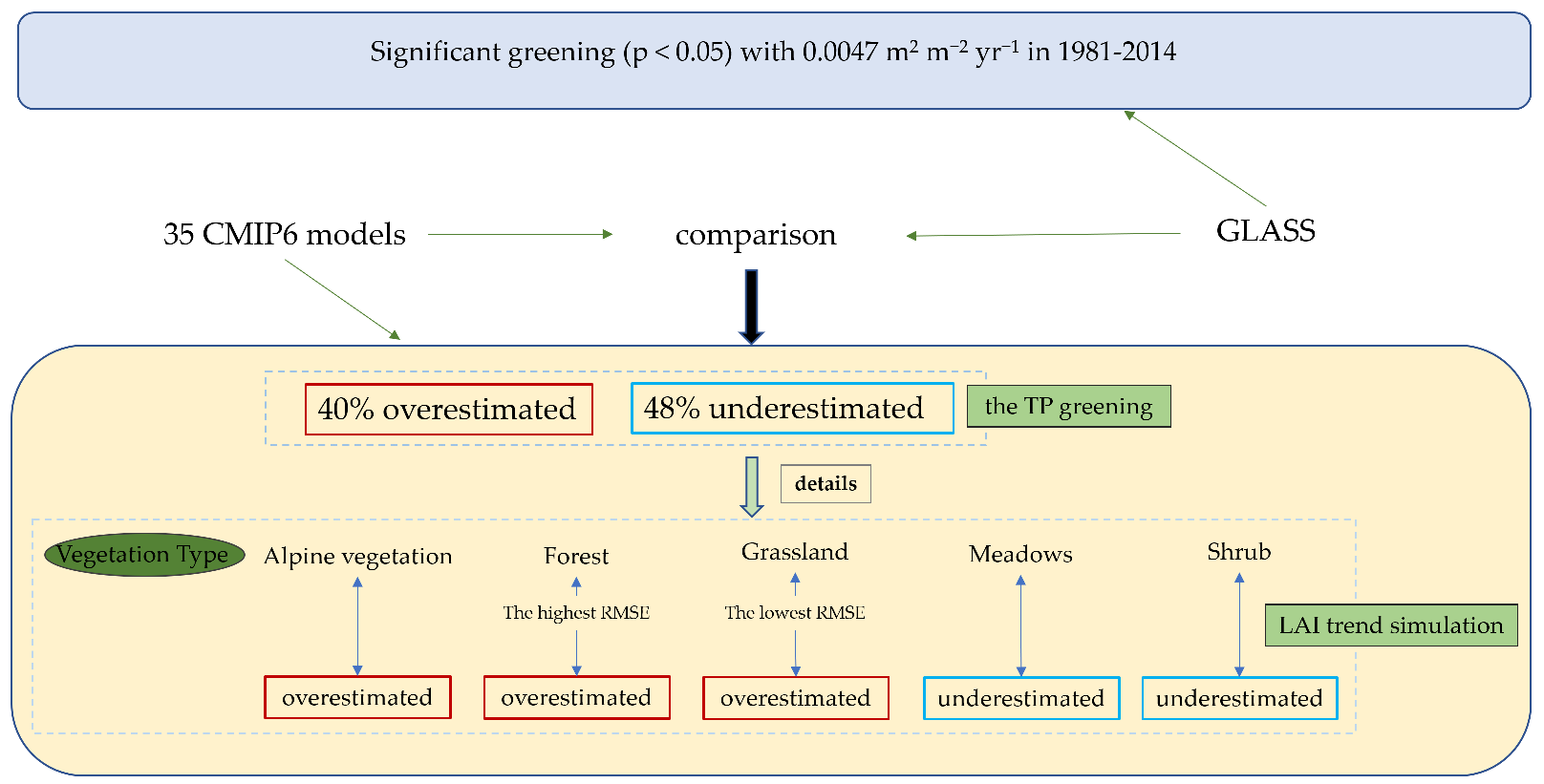
2.1. Study Area
2.2. Satellite Data
2.3. CMIP6 Model Simulations
2.4. Evaluation Approach
2.4.1. Evaluation Metrics
2.4.2. Significant Test Method
2.4.3. Ranking Method
3. Result
3.1. The Average Growing Season LAI and Trend
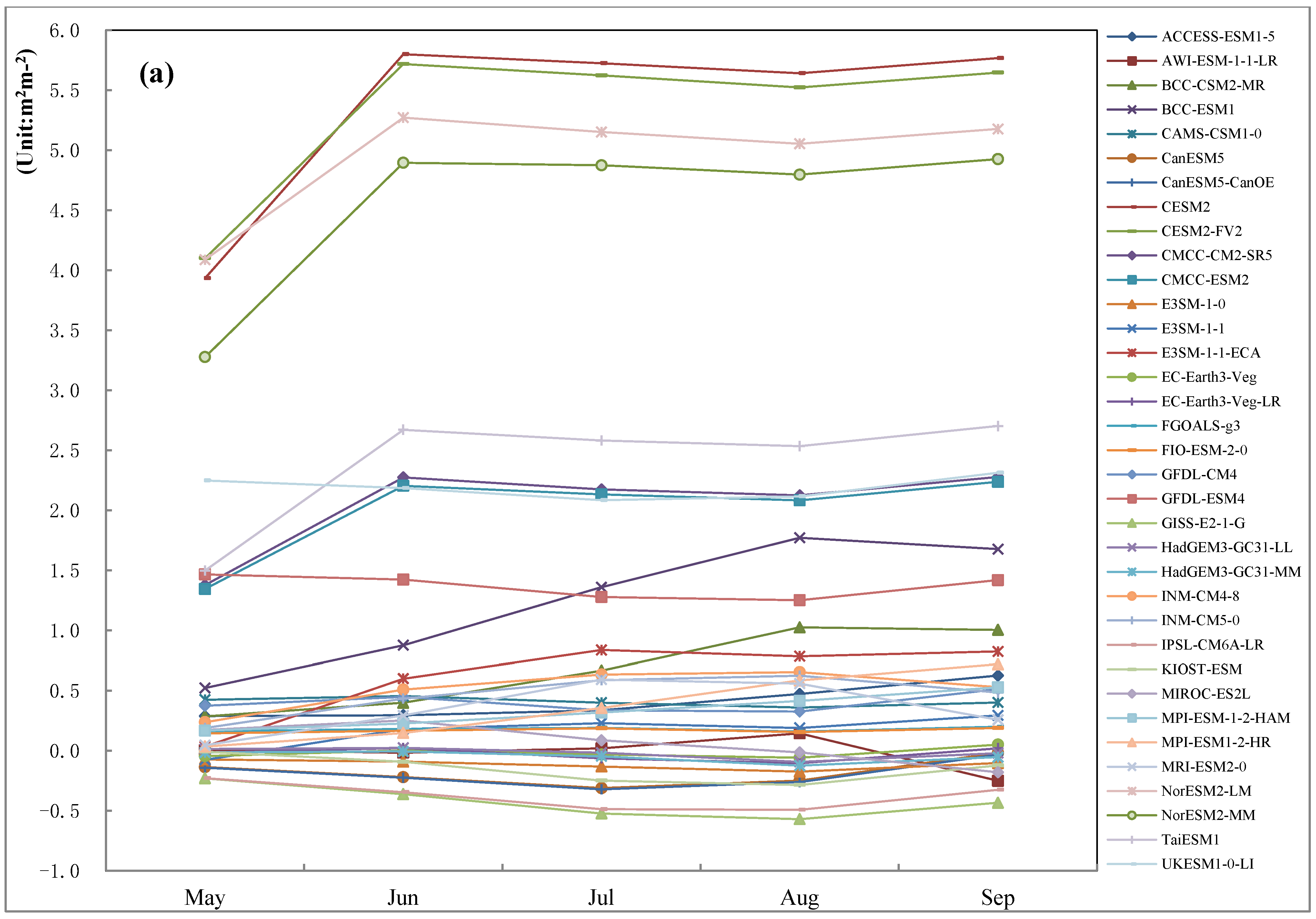
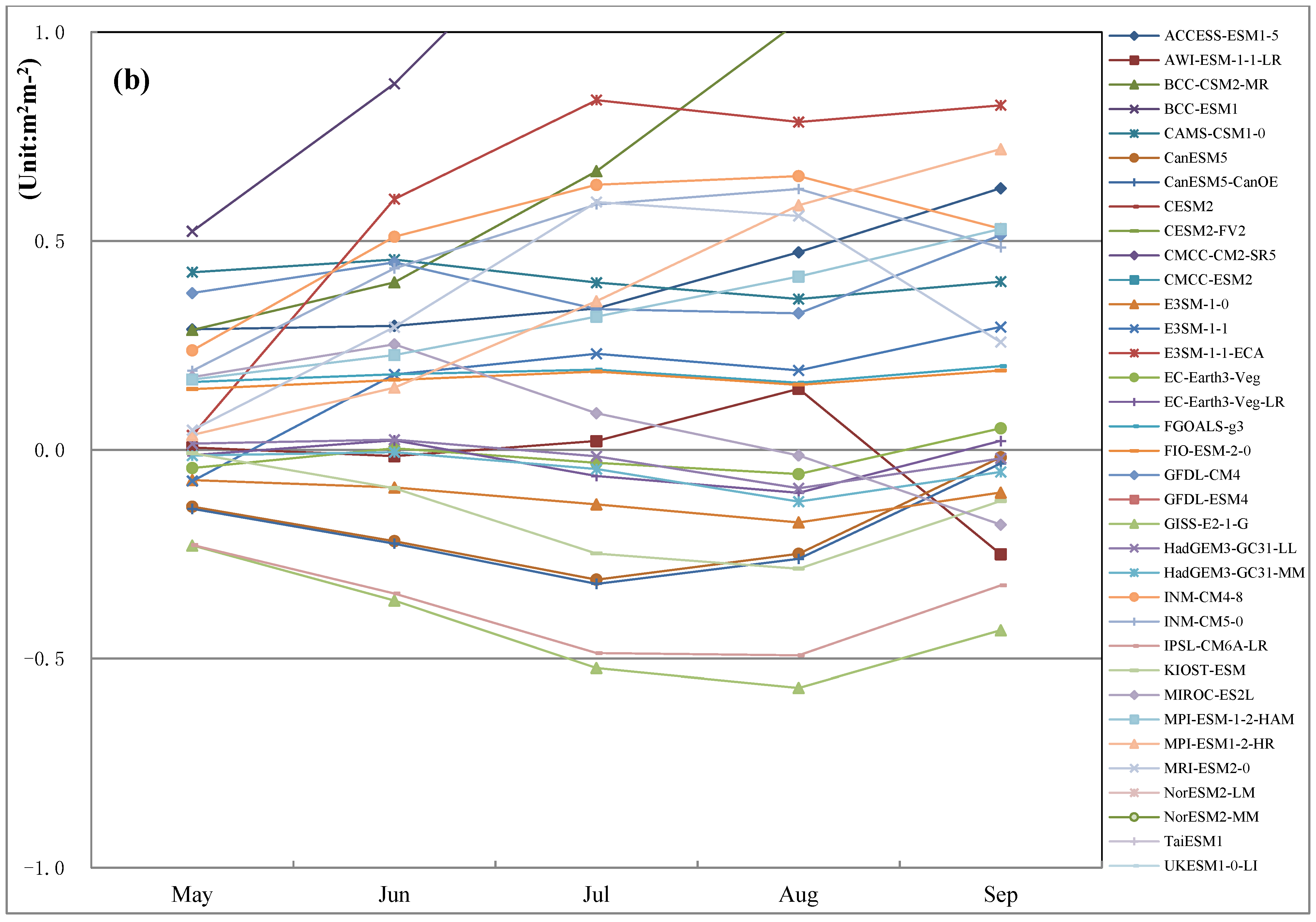
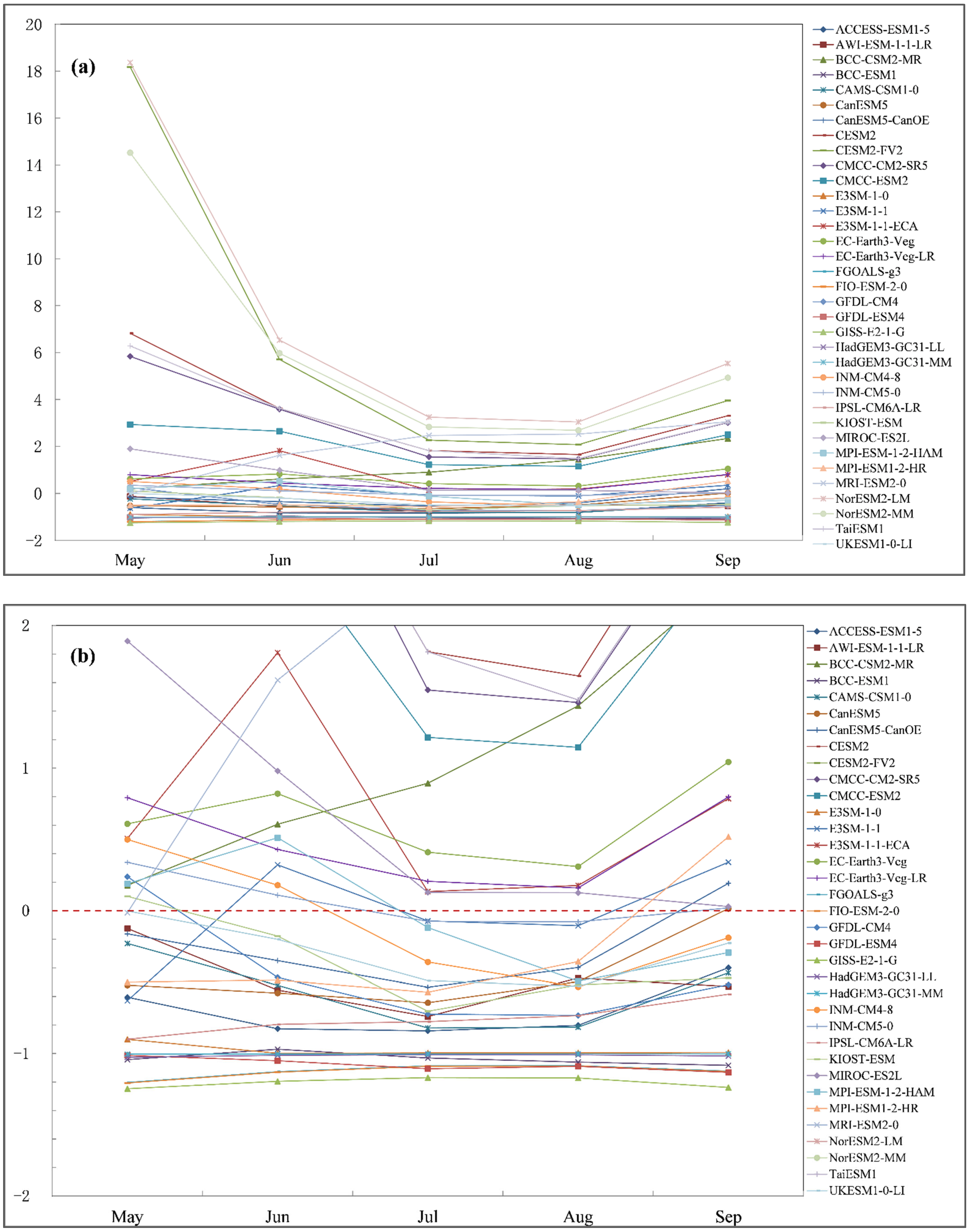
3.2. LAI and Trend Monthly Variations
3.2.1. Monthly Leaf Area Index
3.2.2. Monthly LAI Trend
3.3. LAI Spatial Comparison
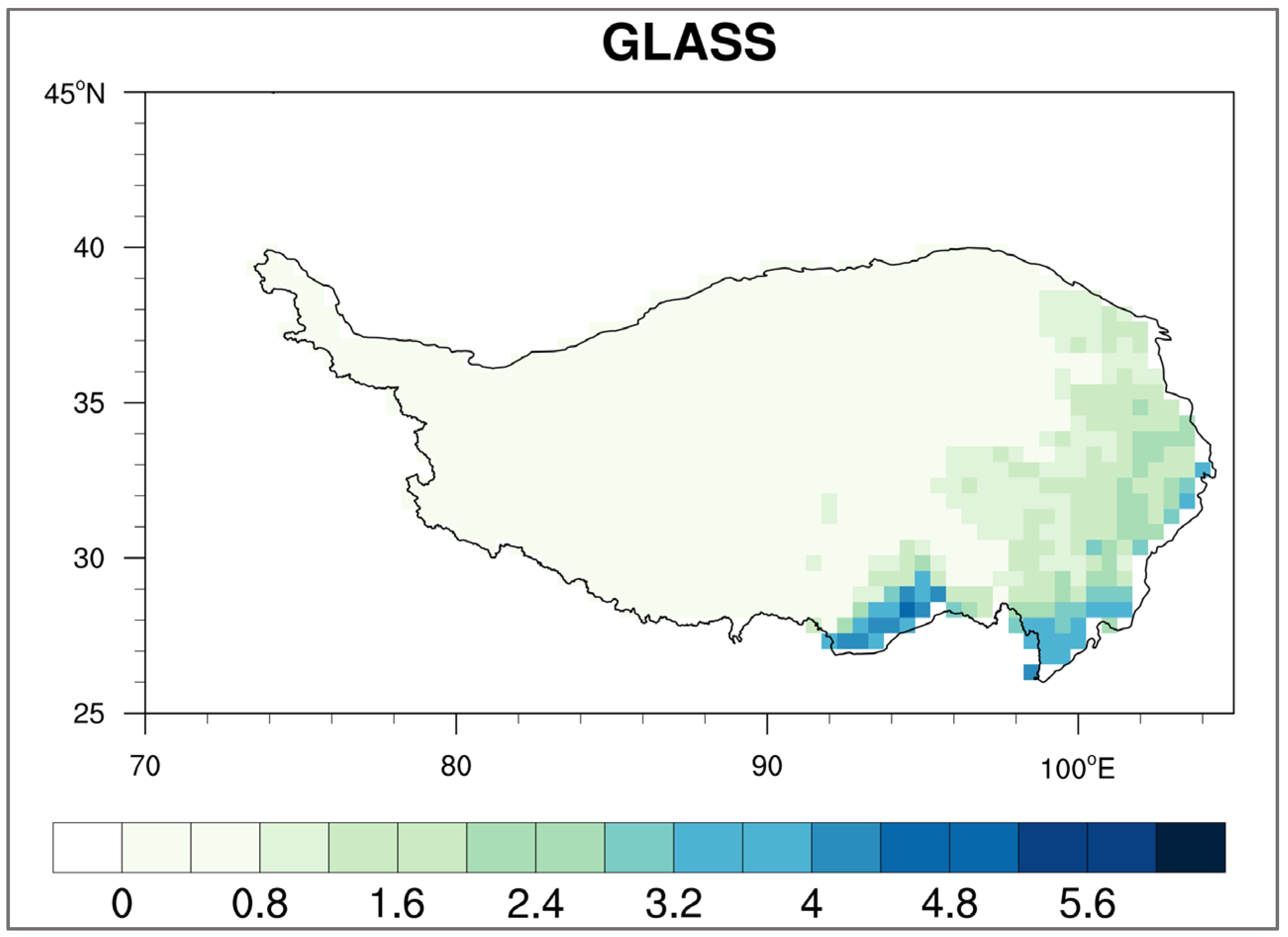
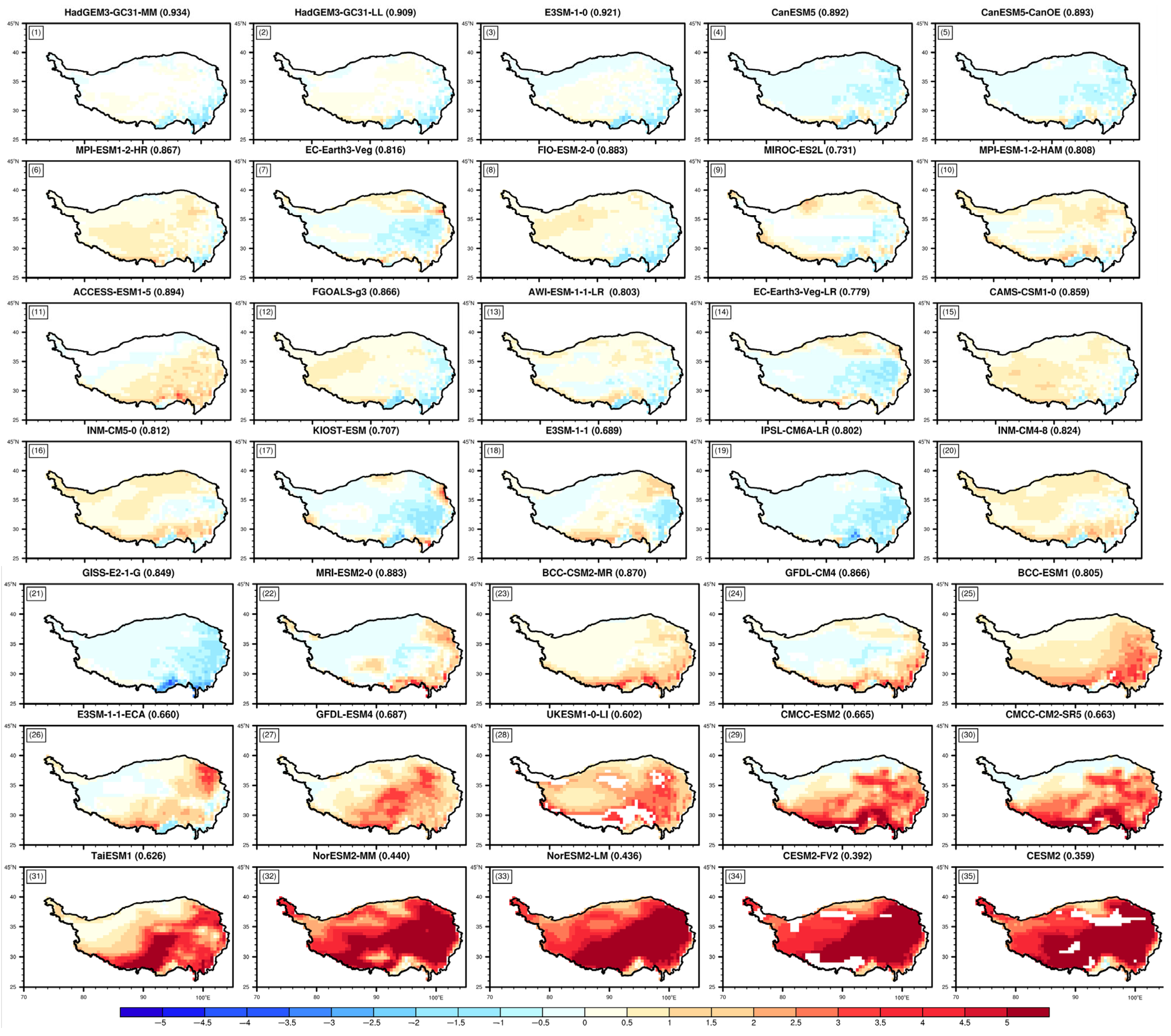
3.3.1. Averaged Leaf Area Index for 1981–2014
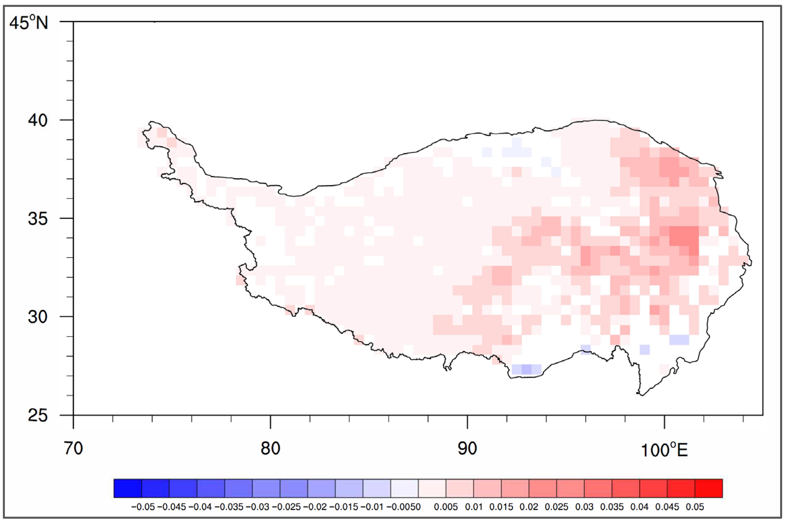
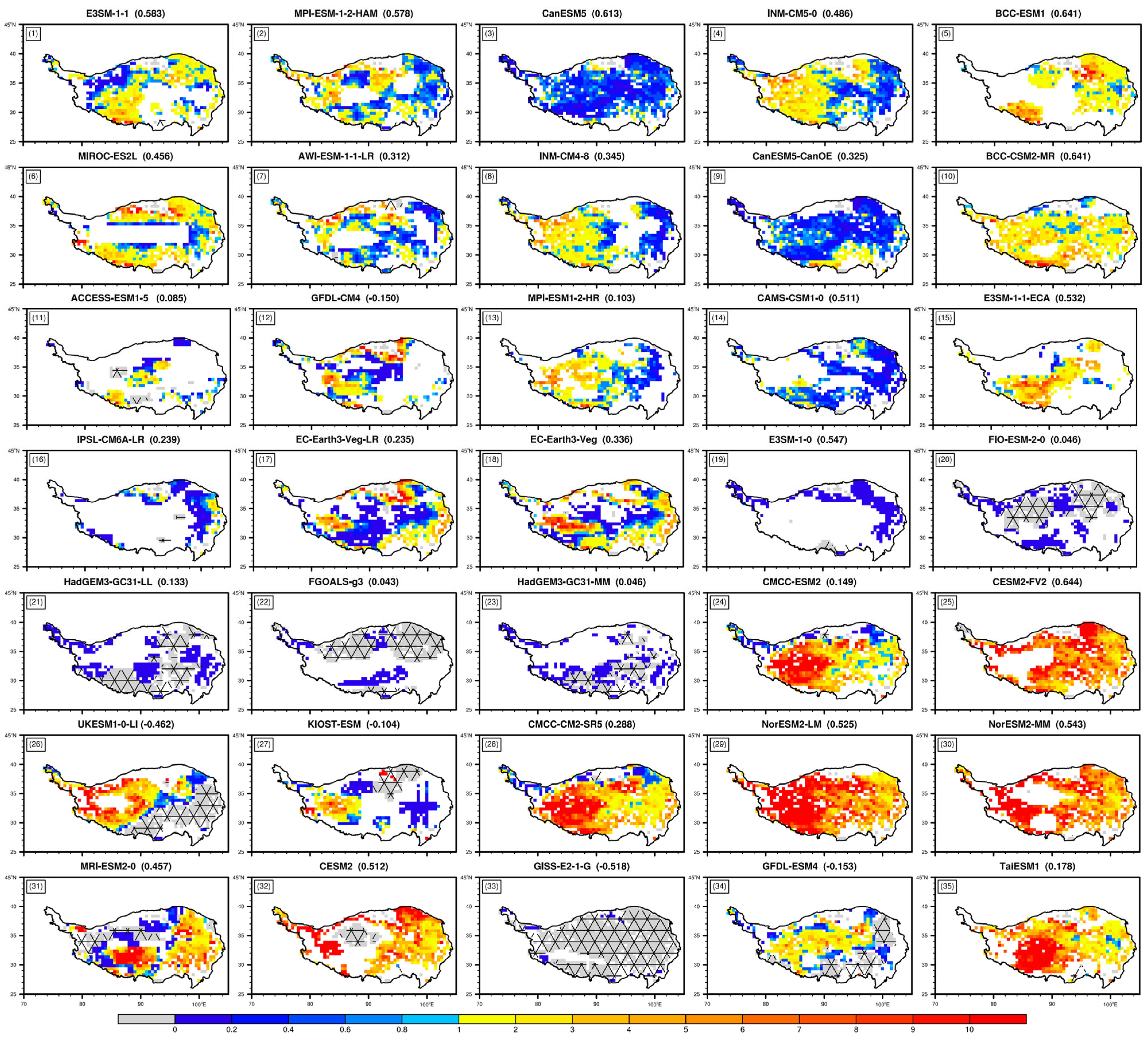
3.3.2. The Leaf Area Index Trend during 1981–2014
4. Discussion
5. Conclusions
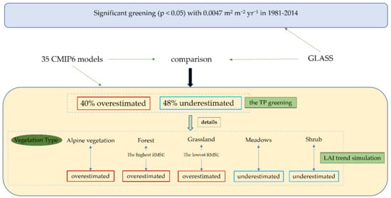
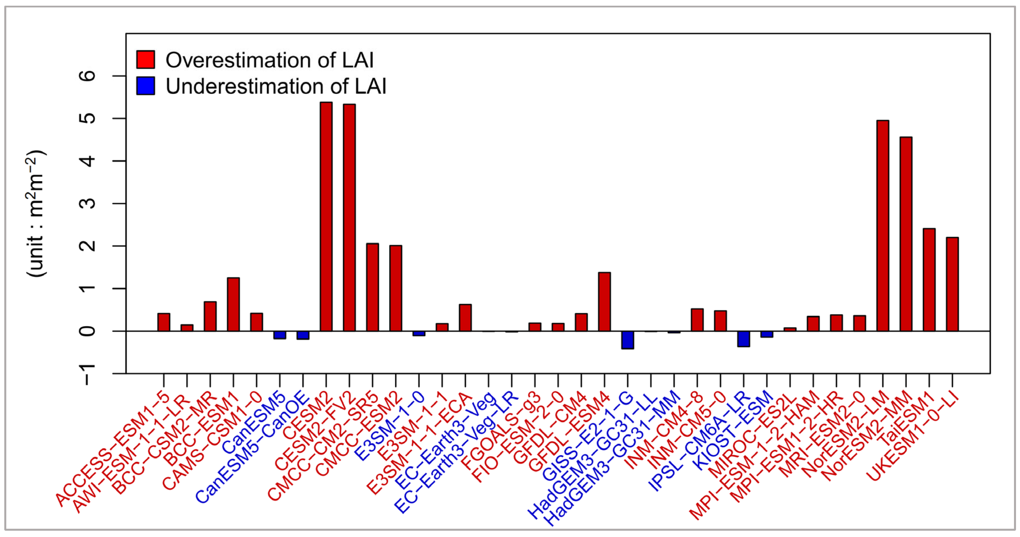
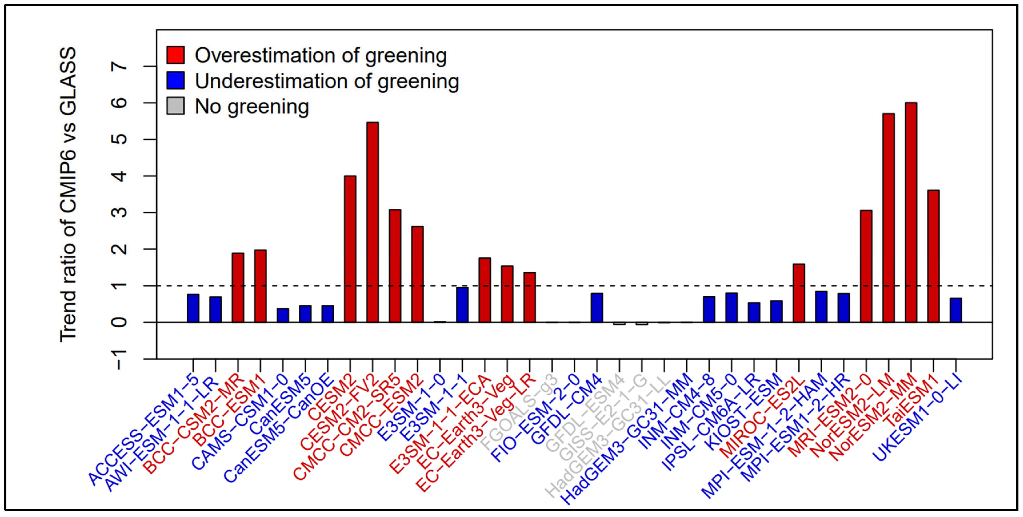
- In total, 40% of the models overestimated the greening, 48% of the models underestimated the greening, and 11% of the models showed a declining LAI trend for 1981–2014 over the Tibetan Plateau. For the LAI, 70% of the models overestimated this, while about 17% of the models underestimated it.
- Both the models underestimating greening, and the models underestimating LAI, showed the greatest underestimation bias in July and August. The biases and ratio of LAI (with the exception of the CLM family) and trend between the simulations and observations had the same change during the growing season.
- CMIP6 models overestimated the LAI trend of alpine vegetation, forest, and grassland, but underestimated the meadow and shrub. The greening of grasslands was overestimated, and the greening of meadows was underestimated in CMIP6. Compared with other vegetation types, the performance of simulating the forest LAI trend was poor with the highest RMSE, and the declining trend in forest pixels showing a declining trend on the TP, was generally underestimated.
- The performance in simulating the spatial distribution of LAI was better than the LAI trend. The underestimation of LAI was mainly in meadows and alpine forest areas in southeast TP. Similar to the forest LAI trend, the simulation performance of forest LAI was also poor, with the highest RMSE, and the forest LAI in parts of the southeast where alpine forests were concentrated on the TP was underestimated by 20 of 35 CMIP6 models.
Supplementary Materials
Author Contributions
Funding
Data Availability Statement
Acknowledgments
Conflicts of Interest
References
- Bonan, G.B. Forests and climate change: Forcings, feedbacks, and the climate benefits of forests. Science 2008, 320, 1444–1449. [Google Scholar] [CrossRef] [PubMed]
- Braswell, B.H.; Schimel, D.S.; Linder, E.; Moore, B. The response of global terrestrial ecosystems to interannual temperature variability. Science 1997, 278, 870–872. [Google Scholar] [CrossRef]
- Nolan, C.; Overpeck, J.T.; Allen, J.R.M.; Anderson, P.M.; Betancourt, J.L.; Binney, H.A.; Brewer, S.; Bush, M.B.; Chase, B.M.; Cheddadi, R.; et al. Past and future global transformation of terrestrial ecosystems under climate change. Science 2018, 361, 920–923. [Google Scholar] [CrossRef]
- Qin, D.; Stocker, T. Highlights of the IPCC Working Group I Fifth Assessment Report. Clim. Change Res. 2014, 10, 1. [Google Scholar]
- Myneni, R.B.; Keeling, C.D.; Tucker, C.J.; Asrar, G.; Nemani, R.R. Increased plant growth in the northern high latitudes from 1981 to 1991. Nature 1997, 386, 698–702. [Google Scholar] [CrossRef]
- Tucker, C.J.; Slayback, D.A.; Pinzon, J.E.; Los, S.O.; Myneni, R.B.; Taylor, M.G. Higher northern latitude normalized difference vegetation index and growing season trends from 1982 to 1999. Int. J. Biometeorol. 2001, 45, 184–190. [Google Scholar] [CrossRef] [PubMed]
- Zhou, L.; Kaufmann, R.K.; Tian, Y.; Myneni, R.B.; Tucker, C.J. Relation between interannual variations in satellite measures of northern forest greenness and climate between 1982 and 1999. J. Geophys. Res.-Atmos. 2003, 108, ACL-3. [Google Scholar] [CrossRef]
- Piao, S.L.; Ciais, P.; Huang, Y.; Shen, Z.H.; Peng, S.S.; Li, J.S.; Zhou, L.P.; Liu, H.Y.; Ma, Y.C.; Ding, Y.H.; et al. The impacts of climate change on water resources and agriculture in China. Nature 2010, 467, 43–51. [Google Scholar] [CrossRef]
- Amagai, Y.; Kudo, G.; Sato, K. Changes in alpine plant communities under climate change: Dynamics of snow-meadow vegetation in northern Japan over the last 40 years. Appl. Veg. Sci. 2018, 21, 561–571. [Google Scholar] [CrossRef]
- Kharuk, V.I.; Im, S.T.; Petrov, I.A. Alpine ecotone in the Siberian Mountains: Vegetation response to warming. J. Mt. Sci. 2021, 18, 3099–3108. [Google Scholar] [CrossRef]
- Jin, Y.H.; Zhang, Y.J.; Xu, J.W.; Tao, Y.; He, H.S.; Guo, M.; Wang, A.L.; Liu, Y.X.; Niu, L.P. Comparative Assessment of Tundra Vegetation Changes Between North and Southwest Slopes of Changbai Mountains, China, in Response to Global Warming. Chin. Geogr. Sci. 2018, 28, 665–679. [Google Scholar] [CrossRef]
- Chen, H.; Zhu, Q.A.; Peng, C.H.; Wu, N.; Wang, Y.F.; Fang, X.Q.; Gao, Y.H.; Zhu, D.; Yang, G.; Tian, J.Q.; et al. The impacts of climate change and human activities on biogeochemical cycles on the Qinghai-Tibetan Plateau. Glob. Change Biol. 2013, 19, 2940–2955. [Google Scholar] [CrossRef] [PubMed]
- Zhang, G.L.; Zhang, Y.J.; Dong, J.W.; Xiao, X.M. Green-up dates in the Tibetan Plateau have continuously advanced from 1982 to 2011. Proc. Natl. Acad. Sci. USA 2013, 110, 4309–4314. [Google Scholar] [CrossRef] [PubMed]
- Duan, A.; Xiao, Z.; Wu, G. Characteristics of Climate Change over the Tibetan Plateau Under the Global Warming During1979—2014. Clim. Change Res. 2016, 12, 374–381. [Google Scholar]
- Gao, J.; Yao, T.D.; Masson-Delmotte, V.; Steen-Larsen, H.C.; Wang, W.C. Collapsing glaciers threaten Asia’s water supplies. Nature 2019, 565, 19–21. [Google Scholar] [CrossRef]
- Wang, S.; Niu, F.; Zhao, L.; Li, S. The thermal stability of roadbed in permafrost regions along Qinghai–Tibet Highway. Cold Reg. Sci. Technol. 2003, 37, 25–34. [Google Scholar] [CrossRef]
- Gao, L.; Liao, J.J.; Shen, G.Z. Monitoring lake-level changes in the Qinghai-Tibetan Plateau using radar altimeter data (2002–2012). J. Appl. Remote Sens. 2013, 7, 073470. [Google Scholar] [CrossRef]
- Liu, J.; Gao, J.; Wang, W. Variations of Vegetation Coverage and Its Relations to Global Climate Changes on the Tibetan Plateau during 1981—2005. J. Mt. Sci. 2013, 31, 234–242. [Google Scholar]
- Wei, Y.; Lu, H.; Wang, J.; Sun, J.; Wang, X. Responses of vegetation zones, in the Qinghai-Tibetan Plateau, to climate change and anthropogenic influences over the last 35 years. Pratac. Sci. 2019, 36, 1163–1176. [Google Scholar]
- Zhang, J.; Yuan, M.S.; Zhang, J.; Li, H.W.; Wang, J.Y.; Zhang, X.; Ju, P.J.; Jiang, H.B.; Chen, H.; Zhu, Q.A. Responses of the NDVI of alpine grasslands on the Qinghai-Tibetan Plateau to climate change and human activities over the last 30 years. Acta Ecol. Sin. 2020, 40, 6269–6281. [Google Scholar]
- Xu, X.; Chen, H.; Levy, J.K. Temporal and spatial changes of vegetation cover characteristics in Qinghai-Tibet Plateau under the background of climate warming And its cause analysis. Chin. Sci. Bull. 2008, 53, 456–462. [Google Scholar]
- Zhang, F.; Tiyip, T.; Ding, J.L.; Sawut, M.; Johnson, V.C.; Tashpolat, N.; Gui, D.W. Vegetation fractional coverage change in a typical oasis region in Tarim River Watershed based on remote sensing. J. Arid Land 2013, 5, 89–101. [Google Scholar] [CrossRef]
- Xiao, Z.Q.; Liang, S.L.; Wang, J.D.; Xiang, Y.; Zhao, X.; Song, J.L. Long-Time-Series Global Land Surface Satellite Leaf Area Index Product Derived From MODIS and AVHRR Surface Reflectance. Ieee Trans. Geosci. Remote Sens. 2016, 54, 5301–5318. [Google Scholar] [CrossRef]
- Liu, Y.; Liu, R.G.; Chen, J.M. Retrospective retrieval of long-term consistent global leaf area index (1981–2011) from combined AVHRR and MODIS data. J. Geophys. Res.-Biogeosci. 2012, 117. [Google Scholar] [CrossRef]
- Zhu, Z.C.; Bi, J.; Pan, Y.Z.; Ganguly, S.; Anav, A.; Xu, L.; Samanta, A.; Piao, S.L.; Nemani, R.R.; Myneni, R.B. Global Data Sets of Vegetation Leaf Area Index (LAI)3g and Fraction of Photosynthetically Active Radiation (FPAR)3g Derived from Global Inventory Modeling and Mapping Studies (GIMMS) Normalized Difference Vegetation Index (NDVI3g) for the Period 1981 to 2011. Remote Sens. 2013, 5, 927–948. [Google Scholar]
- Hua, T.; Wang, X.M. Temporal and Spatial Variations in the Climate Controls of Vegetation Dynamics on the Tibetan Plateau during 1982–2011. Adv. Atmos. Sci. 2018, 35, 1337–1346. [Google Scholar] [CrossRef]
- Zhu, X.C.; Shao, M.G.; Tang, X.Z.; Liang, Y. Spatiotemporal variation and simulation of vegetation coverage in a typical degraded alpine meadow on the Tibetan Plateau. Catena 2020, 190, 104551. [Google Scholar] [CrossRef]
- Lu, J.; Ji, J. A Simulation Study of Atmosphere-Vegetation Interaction over the Tibean Plateau Part II: Net Primary Productivity and Leaf Area Index. Chin. J. Atmos. Sci. 2002, 26, 255–262. [Google Scholar]
- Tian, D.; Guo, Y.; Dong, W.J. Future Changes and Uncertainties in Temperature and Precipitation over China Based on CMIP5 Models. Adv. Atmos. Sci. 2015, 32, 487–496. [Google Scholar] [CrossRef]
- Zhang, F.; Li, W.; Mann, M.E. Scale-dependent regional climate predictability over North America inferred from CMIP3 and CMIP5 ensemble simulations. Adv. Atmos. Sci. 2016, 33, 905–918. [Google Scholar] [CrossRef]
- Xia, J.J.; Yan, Z.W.; Jia, G.S.; Zeng, H.Q.; Jones, P.D.; Zhou, W.; Zhang, A.Z. Projections of the advance in the start of the growing season during the 21st century based on CMIP5 simulations. Adv. Atmos. Sci. 2015, 32, 831–838. [Google Scholar] [CrossRef]
- Anav, A.; Friedlingstein, P.; Kidston, M.; Bopp, L.; Ciais, P.; Cox, P.; Jones, C.; Jung, M.; Myneni, R.; Zhu, Z. Evaluating the Land and Ocean Components of the Global Carbon Cycle in the CMIP5 Earth System Models. J. Clim. 2013, 26, 6801–6843. [Google Scholar] [CrossRef]
- Zhao, Q.; Zhu, Z.; Zeng, H.; Zhao, W.; Myneni, R.B.J.A.; Meteorology, F. Future greening of the Earth may not be as large as previously predicted. Agric. For. Meteorol. 2020, 292, 108111. [Google Scholar] [CrossRef]
- Lawrence, D.M.; Fisher, R.A.; Koven, C.D.; Oleson, K.W.; Swenson, S.C.; Bonan, G.; Collier, N.; Ghimire, B.; van Kampenhout, L.; Kennedy, D.; et al. The Community Land Model Version 5: Description of New Features, Benchmarking, and Impact of Forcing Uncertainty. J. Adv. Model. Earth Syst. 2019, 11, 4245–4287. [Google Scholar] [CrossRef]
- Brovkin, V.; Boysen, L.; Raddatz, T.; Gayler, V.; Loew, A.; Claussen, M. Evaluation of vegetation cover and land-surface albedo in MPI-ESM CMIP5 simulations. J. Adv. Model. Earth Syst. 2013, 5, 48–57. [Google Scholar] [CrossRef]
- Sellar, A.A.; Jones, C.G.; Mulcahy, J.P.; Tang, Y.M.; Yool, A.; Wiltshire, A.; O’Connor, F.M.; Stringer, M.; Hill, R.; Palmieri, J.; et al. UKESM1: Description and Evaluation of the UK Earth System Model. J. Adv. Model. Earth Syst. 2019, 11, 4513–4558. [Google Scholar] [CrossRef]
- Bao, Y.; Gao, Y.H.; Lu, S.H.; Wang, Q.X.; Zhang, S.B.; Xu, J.W.; Li, R.Q.; Li, S.S.; Ma, D.; Meng, X.H.; et al. Evaluation of CMIP5 Earth System Models in Reproducing Leaf Area Index and Vegetation Cover over the Tibetan Plateau. J. Meteorol. Res. 2014, 28, 1041–1060. [Google Scholar] [CrossRef]
- Zhou, T.J.; Zou, L.W.; Chen, X.L. Commentary on the Coupled Model Intercomparison Project Phase 6(CMIP6). Clim. Change Res. 2019, 15, 445. [Google Scholar]
- Watson, D.J. Comparative Physiological Studies on the Growth of Field Crops. 1. Variation in Net Assimilation Rate and Leaf Area between Species and Varieties, and within and between Years. Ann. Bot. 1947, 11, 41–76. [Google Scholar] [CrossRef]
- Wang, L.W.; Niu, Z.; Wei, Y.X. Detecting the areas at risk of desertification in Xinjiang based on modis NDVI imagery. J. Infrared Millim. Waves 2007, 26, 456–460. [Google Scholar]
- Wang, Z.; Liu, S.R.; Sun, P.S.; Guo, Z.H.; Zhou, L.D. The Variability of Vegetation Beginning Date of Greenness Period in Spring in the North-South Transect of Eastern China Based on NOAA NDVI. Spectrosc. Spectr. Anal. 2010, 30, 2758–2761. [Google Scholar]
- Wang, Y.; Tian, Q.J.; Huang, Y.; Wei, H.W. NDVI Difference Rate Recognition Model of Deciduous Broad-Leaved Forest Based on HJ-CCD Remote Sensing Data. Spectrosc. Spectr. Anal. 2013, 33, 1018–1022. [Google Scholar]
- Ewert, F. Modelling plant responses to elevated CO2: How important is leaf area index? Ann. Bot. 2004, 93, 619–627. [Google Scholar] [CrossRef] [PubMed]
- Sellers, P.J.; Dickinson, R.E.; Randall, D.A.; Betts, A.K.; Hall, F.G.; Berry, J.A.; Collatz, G.J.; Denning, A.S.; Mooney, H.A.; Nobre, C.A.; et al. Modeling the exchanges of energy, water, and carbon between continents and the atmosphere. Science 1997, 275, 502–509. [Google Scholar] [CrossRef] [PubMed]
- Zhang, Y.; Liu, L.; Li, B.; Zheng, D. Redetermine the region and boundaries of Tibetan Plateau. Acta Geogr. Res. 2021, 40, 1543–1553. [Google Scholar]
- Zhang, Y.; Liu, L.; Li, B.; Zheng, D. Comparison of boundary datasets covering Tibetan Plateau between 2021 and 2014 versions. J. Glob. Change Data Discov. 2021, 5, 322–332. [Google Scholar]
- Lingzhiduojie, L. Introduction to Environment and Development of Qinghai-Tibet Plateau; China Tibetology Publishing House: Beijing, China, 1996. [Google Scholar]
- Zhang, Y.; Ren, H.; Pan, X. Integration Dataset of Tibet Plateau Boundary; National Tibetan Plateau Data Center: Beijing, China, 2019. [Google Scholar]
- Editorial Committee of Chinese Vegetation Map. Chinese Academy of Sciences. 1:1 Million Vegetation Data Set in China. National Cryosphere Desert Data Center. 2020. Available online: www.ncdc.ac.cn (accessed on 9 December 2021).
- Li, L.; Liu, S.; Zhou, Z.; Zhou, G. Study on Drought Characteristics in Sichuan Province Based on Time Series GLASS LAI Data. Sci. Technol. Assoc. Forum 2013, 123–124. [Google Scholar] [CrossRef]
- Kim, K.; Wang, M.C.; Ranjitkar, S.; Liu, S.H.; Xu, J.C.; Zomer, R.J. Using leaf area index (LAI) to assess vegetation response to drought in Yunnan province of China. J. Mt. Sci. 2017, 14, 1863–1872. [Google Scholar] [CrossRef]
- Li, M.; Du, J.; Li, W.; Li, R.; Wu, S.; Wang, S. Global Vegetation Change and Its Relationship with Precipitation and Temperature Based on GLASS-LAI in 1982–2015. Sci. Geogr. Sin. 2020, 40, 823–832. [Google Scholar]
- Liang, B.; Liu, S. Changes in the Amazon rainforest from 1982 to 2012 using GLASS LAI data. J. Remote Sens. 2016, 20, 149–156. (In Chinese) [Google Scholar]
- Li, X.; Qu, Y. Evaluation of Vegetation Responses to Climatic Factors and Global Vegetation Trends using GLASS LAI from 1982 to 2010. Can. J. Remote Sens. 2018, 44, 357–372. [Google Scholar] [CrossRef]
- Xiao, Z.Q.; Wang, T.T.; Liang, S.L.; Sun, R. Estimating the Fractional Vegetation Cover from GLASS Leaf Area Index Product. Remote Sens. 2016, 8, 337. [Google Scholar] [CrossRef]
- Shi, X.X.; Lohmann, G.; Sidorenko, D.; Yang, H. Early-Holocene simulations using different forcings and resolutions in AWI-ESM. Holocene 2020, 30, 996–1015. [Google Scholar] [CrossRef]
- Ziehn, T.; Lenton, A.; Law, R.M.; Matear, R.J.; Chamberlain, M.A. The carbon cycle in the Australian Community Climate and Earth System Simulator (ACCESS-ESM1)—Part 2: Historical simulations. Geosci. Model Dev. 2017, 10, 2591–2614. [Google Scholar] [CrossRef]
- Wu, T.W.; Lu, Y.X.; Fang, Y.J.; Xin, X.G.; Li, L.; Li, W.P.; Jie, W.H.; Zhang, J.; Liu, Y.M.; Zhang, L.; et al. The Beijing Climate Center Climate System Model (BCC-CSM): The main progress from CMIP5 to CMIP6. Geosci. Model Dev. 2019, 12, 1573–1600. [Google Scholar] [CrossRef]
- Rong, X.Y.; Li, J.; Chen, H.M.; Su, J.Z.; Hua, L.J.; Zhang, Z.Q.; Xin, Y.F. The CMIP6 Historical Simulation Datasets Produced by the Climate System Model CAMS-CSM. Adv. Atmos. Sci. 2021, 38, 285–295. [Google Scholar] [CrossRef]
- Swart, N.C.; Cole, J.N.S.; Kharin, V.V.; Lazare, M.; Scinocca, J.F.; Gillett, N.P.; Anstey, J.; Arora, V.; Christian, J.R.; Hanna, S.; et al. The Canadian Earth System Model version 5 (CanESM50.3). Geosci. Model Dev. 2019, 12, 4823–4873. [Google Scholar] [CrossRef]
- Danabasoglu, G.; Lamarque, J.F.; Bacmeister, J.; Bailey, D.A.; DuVivier, A.K.; Edwards, J.; Emmons, L.K.; Fasullo, J.; Garcia, R.; Gettelman, A.; et al. The Community Earth System Model Version 2 (CESM2). J. Adv. Model. Earth Syst. 2020, 12, e2019MS001916. [Google Scholar] [CrossRef]
- Cherchi, A.; Fogli, P.G.; Lovato, T.; Peano, D.; Iovino, D.; Gualdi, S.; Masina, S.; Scoccimarro, E.; Materia, S.; Bellucci, A.; et al. Global Mean Climate and Main Patterns of Variability in the CMCC-CM2 Coupled Model. J. Adv. Model. Earth Syst. 2019, 11, 185–209. [Google Scholar] [CrossRef]
- Golaz, J.C.; Caldwell, P.M.; van Roekel, L.P.; Petersen, M.R.; Tang, Q.; Wolfe, J.D.; Abeshu, G.; Anantharaj, V.; Asay-Davis, X.S.; Bader, D.C.; et al. The DOE E3SM Coupled Model Version 1: Overview and Evaluation at Standard Resolution. J. Adv. Model. Earth Syst. 2019, 11, 2089–2129. [Google Scholar] [CrossRef]
- Doscher, R.; Acosta, M.; Alessandri, A.; Anthoni, P.; Arsouze, T.; Bergman, T.; Bernardello, R.; Boussetta, S.; Caron, L.P.; Carver, G.; et al. The EC-Earth3 Earth system model for the Coupled Model Intercomparison Project 6. Geosci. Model Dev. 2022, 15, 2973–3020. [Google Scholar] [CrossRef]
- Xie, Z.H.; Liu, S.; Zeng, Y.J.; Gao, J.Q.; Qin, P.H.; Jia, B.H.; Xie, J.B.; Liu, B.; Li, R.C.; Wang, Y.; et al. A High-Resolution Land Model With Groundwater Lateral Flow, Water Use, and Soil Freeze-Thaw Front Dynamics and its Application in an Endorheic Basin. J. Geophys. Res.-Atmos. 2018, 123, 7204–7222. [Google Scholar] [CrossRef]
- Bao, Y.; Song, Z.Y.; Qiao, F.L. FIO-ESM Version 2.0: Model Description and Evaluation. J. Geophys. Res.-Ocean. 2020, 125, e2019JC016036. [Google Scholar] [CrossRef]
- Held, I.M.; Guo, H.; Adcroft, A.; Dunne, J.P.; Horowitz, L.W.; Krasting, J.; Shevliakova, E.; Winton, M.; Zhao, M.; Bushuk, M.; et al. Structure and Performance of GFDL’s CM4.0 Climate Model. J. Adv. Model. Earth Syst. 2019, 11, 3691–3727. [Google Scholar] [CrossRef]
- Dunne, J.P.; Horowitz, L.W.; Adcroft, A.J.; Ginoux, P.; Held, I.M.; John, J.G.; Krasting, J.P.; Malyshev, S.; Naik, V.; Paulot, F.; et al. The GFDL Earth System Model Version 4.1 (GFDL-ESM 4.1): Overall Coupled Model Description and Simulation Characteristics. J. Adv. Model. Earth Syst. 2020, 12, e2019MS002015. [Google Scholar] [CrossRef]
- NASA Goddard Institute for Space Studies (NASA/GISS). NASA-GISS GISS-E2.1G Model Output Prepared for CMIP6 CMIP; Earth System Grid Federation: Washington, DC, USA, 2018. [Google Scholar]
- Walters, D.; Baran, A.J.; Boutle, I.; Brooks, M.; Earnshaw, P.; Edwards, J.; Furtado, K.; Hi, P.; Lock, A.; Manners, J.; et al. The Met Office Unified Model Global Atmosphere 7.0/7.1 and JULES Global Land 7.0 configurations. Geosci. Model Dev. 2019, 12, 1909–1963. [Google Scholar] [CrossRef]
- Volodin, E.M.; Mortikov, E.V.; Kostrykin, S.V.; Galin, V.Y.; Lykossov, V.N.; Gritsun, A.S.; Diansky, N.A.; Gusev, A.V.; Iakovlev, N.G.; Shestakova, A.A.; et al. Simulation of the modern climate using the INM-CM48 climate model. Russ. J. Numer. Anal. Math. Model. 2018, 33, 367–374. [Google Scholar] [CrossRef]
- Volodin, E.M.; Mortikov, E.V.; Kostrykin, S.V.; Galin, V.Y.; Lykossov, V.N.; Gritsun, A.S.; Diansky, N.A.; Gusev, A.V.; Iakovlev, N.G. Simulation of the present-day climate with the climate model INMCM5. Clim. Dyn. 2017, 49, 3715–3734. [Google Scholar]
- Boucher, O.; Servonnat, J.; Albright, A.L.; Aumont, O.; Balkanski, Y.; Bastrikov, V.; Bekki, S.; Bonnet, R.; Bony, S.; Bopp, L.; et al. Presentation and Evaluation of the IPSL-CM6A-LR Climate Model. J. Adv. Model. Earth Syst. 2020, 12, e2019MS002010. [Google Scholar] [CrossRef]
- Milly, P.C.D.; Malyshev, S.L.; Shevliakova, E.; Dunne, K.A.; Findell, K.L.; Gleeson, T.; Liang, Z.; Phillipps, P.; Stouffer, R.J.; Swenson, S. An Enhanced Model of Land Water and Energy for Global Hydrologic and Earth-System Studies. J. Hydrometeorol. 2014, 15, 1739–1761. [Google Scholar] [CrossRef]
- Hajima, T.; Watanabe, M.; Yamamoto, A.; Tatebe, H.; Noguchi, M.A.; Abe, M.; Ohgaito, R.; Ito, A.; Yamazaki, D.; Okajima, H.; et al. Development of the MIROC-ES2L Earth system model and the evaluation of biogeochemical processes and feedbacks. Geosci. Model Dev. 2020, 13, 2197–2244. [Google Scholar] [CrossRef]
- Mauritsen, T.; Bader, J.; Becker, T.; Behrens, J.; Bittner, M.; Brokopf, R.; Brovkin, V.; Claussen, M.; Crueger, T.; Esch, M.; et al. Developments in the MPI-M Earth System Model version 1.2 (MPI-ESM1.2) and Its Response to Increasing CO2. J. Adv. Model. Earth Syst. 2019, 11, 998–1038. [Google Scholar] [CrossRef]
- Yukimoto, S.; Kawai, H.; Koshiro, T.; Oshima, N.; Yoshida, K.; Urakawa, S.; Tsujino, H.; Deushi, M.; Tanaka, T.; Hosaka, M.; et al. The Meteorological Research Institute Earth System Model Version 2.0, MRI-ESM2.0: Description and Basic Evaluation of the Physical Component. J. Meteorol. Soc. Jpn. 2019, 97, 931–965. [Google Scholar] [CrossRef]
- Seland, O.; Bentsen, M.; Olivie, D.; Toniazzo, T.; Gjermundsen, A.; Graff, L.S.; Debernard, J.B.; Gupta, A.K.; He, Y.C.; Kirkevag, A.; et al. Overview of the Norwegian Earth System Model (NorESM2) and key climate response of CMIP6 DECK, historical, and scenario simulations. Geosci. Model Dev. 2020, 13, 6165–6200. [Google Scholar] [CrossRef]
- Lee, W.L.; Wang, Y.C.; Shiu, C.J.; Tsai, I.C.; Tu, C.Y.; Lan, Y.Y.; Chen, J.P.; Pan, H.L.; Hsu, H.H. Taiwan Earth System Model Version 1: Description and evaluation of mean state. Geosci. Model Dev. 2020, 13, 3887–3904. [Google Scholar] [CrossRef]
- Chang, Q.; Dou, J. Exploration on Spatial Correlation of Two Space Variables. Stat. Appl. 2016, 5, 397–403. [Google Scholar]
- Brunke, M.A.; Fairall, C.W.; Zeng, X.B.; Eymard, L.; Curry, J.A. Which bulk aerodynamic algorithms are least problematic in computing ocean surface turbulent fluxes? J. Clim. 2003, 16, 619–635. [Google Scholar] [CrossRef]
- Decker, M.; Brunke, M.A.; Wang, Z.; Sakaguchi, K.; Zeng, X.B.; Bosilovich, M.G. Evaluation of the Reanalysis Products from GSFC, NCEP, and ECMWF Using Flux Tower Observations. J. Clim. 2012, 25, 1916–1944. [Google Scholar] [CrossRef]
- Wang, A.H.; Zeng, X.B. Evaluation of multireanalysis products with in situ observations over the Tibetan Plateau. J. Geophys. Res.-Atmos. 2012, 117. [Google Scholar] [CrossRef]
- Sun, C.; Liu, L.; Guan, L. Validation of the GLASS LAI products in Xilinhot Grassland. Remote Sens. Technol. Appl. 2013, 28, 949–954. [Google Scholar]
- Xiang, Y.; Xiao, Z.; Liang, S.; Wang, J.; Song, J. Validation of Global LAnd Surface Satellite (GLASS) leaf area index product. J. Remote Sens. 2014, 18, 573–596. [Google Scholar]
- Xu, X.Y.; Riley, W.J.; Koven, C.D.; Jia, G.S.; Zhang, X.Y. Earlier leaf-out warms air in the north. Nat. Clim. Change 2020, 10, 370–375. [Google Scholar] [CrossRef]
- Yu, H.Y.; Luedeling, E.; Xu, J.C. Winter and spring warming result in delayed spring phenology on the Tibetan Plateau. Proc. Natl. Acad. Sci. USA 2010, 107, 22151–22156. [Google Scholar] [CrossRef] [PubMed]
- Shen, M.G.; Sun, Z.Z.; Wang, S.P.; Zhang, G.X.; Kong, W.D.; Chen, A.P.; Piao, S.L. No evidence of continuously advanced green-up dates in the Tibetan Plateau over the last decade. Proc. Natl. Acad. Sci. USA 2013, 110, E2329. [Google Scholar] [CrossRef] [PubMed]
- Wang, T.; Peng, S.S.; Lin, X.; Chang, J.F. Declining snow cover may affect spring phenological trend on the Tibetan Plateau. Proc. Natl. Acad. Sci. USA 2013, 110, E2854–E2855. [Google Scholar] [CrossRef] [PubMed]
- Chen, B.X.; Zhang, X.Z.; Tao, J.; Wu, J.S.; Wang, J.S.; Shi, P.L.; Zhang, Y.J.; Yu, C.Q. The impact of climate change and anthropogenic activities on alpine grassland over the Qinghai-Tibet Plateau. Agric. For. Meteorol. 2014, 189, 11–18. [Google Scholar] [CrossRef]
- Piao, S.L.; Cui, M.D.; Chen, A.P.; Wang, X.H.; Ciais, P.; Liu, J.; Tang, Y.H. Altitude and temperature dependence of change in the spring vegetation green-up date from 1982 to 2006 in the Qinghai-Xizang Plateau. Agric. For. Meteorol. 2011, 151, 1599–1608. [Google Scholar] [CrossRef]
- Shen, M.G.; Piao, S.L.; Jeong, S.J.; Zhou, L.M.; Zeng, Z.Z.; Ciais, P.; Chen, D.L.; Huang, M.T.; Jin, C.S.; Li, L.Z.X.; et al. Evaporative cooling over the Tibetan Plateau induced by vegetation growth. Proc. Natl. Acad. Sci. USA 2015, 112, 9299–9304. [Google Scholar] [CrossRef]
- Xin, X.; Wu, T.; Zhang, J. Introduction of BCC models and its participation in CMIP6. Clim. Change Res. 2019, 15, 533–539. [Google Scholar]
- Song, Z.Y.; Bao, Y.; Qiao, F.L. Introduction of FIO-ESM v2.0 and its participation plan in CMIP6 experiments. Clim. Change Res. 2019, 15, 558. [Google Scholar]
- Wang, Y.C.; Hsu, H.H.; Chen, C.A.; Tseng, W.L.; Hsu, P.C.; Lin, C.W.; Chen, Y.L.; Jiang, L.C.; Lee, Y.C.; Liang, H.C.; et al. Performance of the Taiwan Earth System Model in Simulating Climate Variability Compared With Observations and CMIP6 Model Simulations. J. Adv. Model. Earth Syst. 2021, 13, e2020MS002353. [Google Scholar] [CrossRef]
- Keeble, J.; Hassler, B.; Banerjee, A.; Checa-Garcia, R.; Chiodo, G.; Davis, S.; Eyring, V.; Griffiths, P.T.; Morgenstern, O.; Nowack, P.; et al. Evaluating stratospheric ozone and water vapour changes in CMIP6 models from 1850 to 2100. Atmos. Chem. Phys. 2021, 21, 5015–5061. [Google Scholar] [CrossRef]
- Burrows, S.M.; Maltrud, M.; Yang, X.; Zhu, Q.; Jeffery, N.; Shi, X.; Ricciuto, D.; Wang, S.; Bisht, G.; Tang, J.; et al. The DOE E3SM v1.1 Biogeochemistry Configuration: Description and Simulated Ecosystem-Climate Responses to Historical Changes in Forcing. J. Adv. Model. Earth Syst. 2020, 12, e2019MS001766. [Google Scholar] [CrossRef]
- Andrews, M.B.; Ridley, J.K.; Wood, R.A.; Andrews, T.; Blockley, E.W.; Booth, B.; Burke, E.; Dittus, A.J.; Florek, P.; Gray, L.J.; et al. Historical Simulations With HadGEM3-GC3.1 for CMIP6. J. Adv. Model. Earth Syst. 2020, 12, e2019MS001995. [Google Scholar] [CrossRef]
- Sellar, A.A.; Walton, J.; Jones, C.G.; Wood, R.; Abraham, N.L.; Andrejczuk, M.; Andrews, M.B.; Andrews, T.; Archibald, A.T.; de Mora, L.; et al. Implementation of UK Earth System Models for CMIP6. J. Adv. Model. Earth Syst. 2020, 12, e2019MS001946. [Google Scholar] [CrossRef]
- Luo, L.; Zhang, Y.; Zhou, J.; Pan, X.; Sun, W. Simulation and application of the land surface model CLM Drive by WRF in the Tibetan Plateau. J. Glaciol. Geocryol. 2013, 35, 553–564. (In Chinese) [Google Scholar]
- Xiong, J.; Zhang, Y.; Wang, S. Influence of soil moisture transmission scheme improvement in CLM4.0 on simulation of land surface process in Qinghai-Xizang Plateau. Plateau Meteorol. 2014, 33, 323–336. (In Chinese) [Google Scholar]
- Xie, Z.; Hu, Z.; Liu, H.; Sun, G.; Yang, Y.; Lin, Y.; Huang, F. Evaluation of the surface energy exchange simulations of land surface model CLM4.5 in alpine meadow over the Qinghai-Xizang Plateau. Plateau Meteorol. 2017, 36, 1–12. (In Chinese) [Google Scholar]
- Song, Y.; Fan, Y.; Ma, T. Evaluation of simulation performance of land surface model NCAR_CLM4.5 at a degrated glassland station in semi-arid area. Trans. Atmos. Sci. 2014, 37, 794–803. (In Chinese) [Google Scholar]
- Mao, J.F.; Thornton, P.E.; Shi, X.Y.; Zhao, M.S.; Post, W.M. Remote Sensing Evaluation of CLM4 GPP for the Period 2000–09. J. Clim. 2012, 25, 5327–5342. [Google Scholar] [CrossRef]
- Song, X.; Wang, D.Y.; Li, F.; Zeng, X.D. Evaluating the performance of CMIP6 Earth system models in simulating global vegetation structure and distribution. Adv. Clim. Change Res. 2021, 12, 584–595. [Google Scholar] [CrossRef]
- Yang, Y.; Piao, S. Variation in grassland vegetation cover in relation to climatic factors on the Tibetan Plateau. Chin. J. Plant Ecol. 2006, 30, 1. (In Chinese) [Google Scholar]
- Yu, H.; Xu, J. Effects of climate change on vegetations on Qinghai-Tibet Plateau: A review. Chin. J. Ecol. 2009, 28, 747–754. (In Chinese) [Google Scholar]
- Yang, J.; Ding, Y.; Shen, Y.; Liu, S.; Chen, R. Climatic Features of Eco-Environment Change in the Source Regions of the Yangtze and Yellow Rivers in Recent 40 Years. J. Glaciol. Geocryol. 2004, 26, 7–16. (In Chinese) [Google Scholar]
- Wang, Y.; Zhao, Z.; Qiao, Y.; Li, C. Characteristics of the climatic variatation in zoig(e) in the past 45 years and its effects on the eco-environment in the area. J. Geomech. 2005, 11, 328–332, 340. [Google Scholar]
- Li, Y.; Zhao, L.; Zhao, X.; Zhou, H. Effects of a 5-years mimic Temperature Increase to the structure and productivity of kobresia humilis meadow. Acta Agrestia Sin. 2004, 12, 236–239. [Google Scholar]
- Wang, S.; Zhao, L.; Li, S. Interaction between Permafrost and Desertification on the Qinghai-Tibet Plateau. J. Desert Res. 2002, 22, 33–39. [Google Scholar]
- Zhang, J.; Fu, C.; Yan, X.; Seita, E.; Hiroshi, K. Global respondence analysis of LAI versus surface air temperature and precipitation variation. Chin. J. Geophys. 2002, 45, 631–637. (In Chinese) [Google Scholar] [CrossRef]
- Zhu, X.D.; He, H.L.; Liu, M.; Yu, G.R.; Sun, X.M.; Gao, Y.H. Spatio-temporal variation of photosynthetically active radiation in China in recent 50 years. J. Geogr. Sci. 2010, 20, 803–817. [Google Scholar] [CrossRef]
- Fan, S.; Fan, G.; Lai, X. Analysis on variation trend of season start dates over the Tibetan Plateau during 1961–2007. Clim. Environ. Res. 2013, 18, 71–79. (In Chinese) [Google Scholar]
- Wu, K.; Liu, S.; Bao, W.; Wang, R. Remote sensing monitoring of the glacier change in the Gangrigabu Range, southeast Tibetan Plateau from 1980 through 2015. J. Glaciol. Geocryol. 2017, 39, 24–34. [Google Scholar]
- Xia, L.; Song, X.; Cai, S.; Hu, R.; Guo, D. Role of surface hydrothermal elements in grassland degradation over the Tibetan Plateau. Acta Ecol. Sin. 2021, 41, 4618–4631. [Google Scholar]
- Feng, Q.; Gao, X.; Huang, X.; Yu, H.; Liang, T. Remote sensing dynamic monitoring of grass growth in Qinghai-Tibet plateau from 2001 to 2010. J. Lanzhou Univ. 2011, 47, 75–81, 90. [Google Scholar]
- Xiao, Y.; Li, J.; Li, N. Evaluation of CMIP6 HighResMIP models in Simulating Precipitation over Tibetan Plateau. Torrential Rain Disasters 2022, 41, 215–223. (In Chinese) [Google Scholar]
- Chen, W.; Jiang, D.; Wang, X. Evaluation and Projection of CMIP6 Models for Climate over the Qinghai-Xizang (Tibetan) Plateau. Plateau Meteorol. 2021, 40, 1455–1469. (In Chinese) [Google Scholar]
- Luo, S.; Lv, S.; Zhang, Y. Simulation analysis on land surface process of BJ site of Central Tibetan Plateau using CoLM. Plateau Meteorol. 2008, 27, 259–271. (In Chinese) [Google Scholar]
- Yang, Y.; Li, M.; Hu, Z. Influence of surface roughness on surface-air fluxes in alpine meadow over the Northern Qinghai-Xizang Plateau. Plateau Meteorol. 2014, 33, 626–636. (In Chinese) [Google Scholar]
- Gao, Z.; Chae, N.; Kim, J. Modeling of surface energy partitioning, surace temperature, and soil wetness in the Tibetan prairie using the Simple Biosphere Model 2 (SiB2). J. Geophys. Res. Atmos. 2004, 109, D06102. [Google Scholar] [CrossRef]
- Swingedouw, D.; Mignot, J.; Ortega, P.; Khodri, M.; Menegoz, M.; Cassou, C.; Hanquiez, V. Impact of explosive volcanic eruptions on the main climate variability modes. Glob. Planet. Change 2017, 150, 24–45. [Google Scholar] [CrossRef]
- Singh, M.; Krishnan, R.; Goswami, B.; Choudhury, A.D.; Swapna, P.; Vellore, R.; Prajeesh, A.G.; Sandeep, N.; Venkataraman, C.; Donner, R.V.; et al. Fingerprint of volcanic forcing on the ENSO-Indian monsoon coupling. Sci. Adv. 2020, 6, eaba8164. [Google Scholar] [CrossRef]
- Ma, X.; Chen, S.; Deng, J.; Feng, Q.; Huang, X. Vegetation Phenology dynamics and its response to climate change on the Tibetan Plateau. Acta Ecol. Sin. 2016, 25, 13–21. [Google Scholar]


| Model | Institute | Land Surface Model | Resolution | Reference |
|---|---|---|---|---|
| AWI-ESM-1-1-LR | AWI (Germany) | CABLE2.4 | 250 km | [56] |
| ACCESS-ESM1-5 | CSIRO (Australia) | CABLE2.4 | 250 km | [57] |
| BCC-CSM2-MR | BCC (China) | BCC-AVIM2.0 | 100 km | [58] |
| BCC-ESM1 | BCC (China) | BCC-AVIM2.0 | 250 km | [58] |
| CAMS-CSM1-0 | China | CoLM | 100 km | [59] |
| CanESM5 | CCCMA (Canada) | CLASS3.6-CTEM1.2 | 500 km | [60] |
| CanESM5-CanOE | CCCMA (Canada) | CLASS3.6-CTEM1.2 | 500 km | [60] |
| CESM2 | NCAR (USA) | CLM5 | 100 km | [61] |
| CESM2-FV2 | NCAR (USA) | CLM5 | 100 km | [61] |
| CMCC-CM2-SR5 | CMCC (Italy) | CLM4.5 | 100 km | [62] |
| CMCC-ESM2 | CMCC (Italy) | CLM4.5 | 100 km | [62] |
| E3SM-1-0 | E3SM-Project (USA) | ELM | 100 km | [63] |
| E3SM-1-1 | E3SM-Project (USA) | ELM | 100 km | [63] |
| E3SM-1-1-ECA | E3SM-Project (USA) | ELM | 100 km | [63] |
| EC-Earth3-Veg | EC-Earth-Consortium (Europe) | HTESSEL | 100 km | [64] |
| EC-Earth3-Veg-LR | EC-Earth-Consortium (Europe) | HTESSEL | 100 km | [64] |
| FGOALS-g3 | China | CAS-LSM | 2 × 2° | [65] |
| FIO-ESM-2-0 | FIO (China) | CLM4.0 | 100 km | [66] |
| GFDL-CM4 | GFDL (USA) | LM4.0 | 100 km | [67] |
| GFDL-ESM4 | GFDL (USA) | LM4.1 | 100 km | [68] |
| GISS-E2-1-G | GISS (USA) | GISS LSM | 250 km | [69] |
| HadGEM3-GC31-LL | HadGEM (United Kingdom) | JULES | 250 km | [70] |
| HadGEM3-GC31-MM | HadGEM (United Kingdom) | JULES | 100 km | [70] |
| INM-CM4-8 | INM (Russia) | INM-LND1 | 100 km | [71] |
| INM-CM5-0 | INM (Russia) | INM-LND1 | 100 km | [72] |
| IPSL-CM6A-LR | IPSL (France) | ORCHIDEE v2 | 250 km | [73] |
| KIOST-ESM | KIOST (Korea) | LM3.0 | 250 km | [74] |
| MIROC-ES2L | MIROC (Japan) | MATSIRO6.0 +VISIT-e v1 | 500 km | [75] |
| MPI-ESM-1-2-HAM | HAMMOZ Consortium (Switzerland, Germany, Finland, UK) | CABLE2.4 | 250 km | [76] |
| MPI-ESM1-2-HR | MPI (Germany) | CABLE2.4 | 100 km | [76] |
| MRI-ESM2-0 | MRI (Japan) | HAL 1.0 | 100 km | [77] |
| NorESM2-LM | NCC (Norway) | CLM5 | 250 km | [78] |
| NorESM2-MM | NCC (Norway) | CLM5 | 100 km | [78] |
| TaiESM1 | AS-RCEC (Taiwan, China) | CLM4.0 | 100 km | [79] |
| UKESM1-0-LI | MOHC (UK) | JULES-ES-1.0 | 250 km | [36] |
| Land Surface Model | CMIP6 Models | The Difference of Models |
|---|---|---|
| BCC-AVIM2.0 | BCC-CSM2-MR | BCC-CSM2-MR uses the carbon emissions provided by CMIP6 as the forcing, but BCC-ESM1.0 uses the chemical reaction gas and aerosol emission data provided by CMIP6 as the forcing [93] |
| BCC-ESM1 | ||
| CLASS3.6-CTEM1.2 | CanESM5 | CanESM5-CanOE is exactly the same physical model as CanESM5, but it couples it with the CanOE ocean biogeochemical model [60] |
| CanESM5-CanOE | ||
| CLM4.0 | FIO-ESM-2-0 | The FIO-ESM-2-0 model adds an ocean surface wave model to the traditional atmosphere–land–ocean–sea ice coupled model of CPL7; TaiESM1 was developed on the basis of the Community Earth System Model version 1.2.2 by implementing several improvements to the parameterization schemes in the atmospheric component [94,95] |
| TaiESM1 | ||
| CLM4.5 | CMCC-CM2-SR5 | CMCC-CM2-SR5 does not include ocean biogeochemistry model in the model, but the BFM5.1 ocean biogeochemistry model was added to CMCC-ESM2 |
| CMCC-ESM2 | ||
| CLM5.0 | CESM2 CESM2-FV2 NorESM2-LM NorESM2-MM | CESM2-FV2 reduces the horizontal resolution of the atmosphere and land on the basis of CESM2; NorESM2-LM and NorESM2-MM are similar to the CESM2 and CESM2-FV2 models in terms of the framework and model composition; the differences are that NorESM2 uses completely different oceans and oceano-biogeochemical model and uses a different ocean and oceano-biogeochemistry model and the atmosphere component of NorESM2-MM and CAM-Nor; the difference between NorESM2-LM and NorESM2-MM is the resolution [78,96] |
| ELM | E3SM-1-0 E3SM-1-1 E3SM-1-1-ECA | On the basis of E3SM-1-0, E3SM-1-1 has corrected several vulnerabilities and made improvements; on the basis of E3SM-1-1, E3SM-1-1-ECA uses the ECA plant and soil carbon and nutrient mechanisms, soil carbon and the effects of nutrients representing carbon, nitrogen and phosphorus, and it excludes the effect of coupled ocean and sea ice biogeochemistry [97] |
| HTESSEL | EC-Earth3-Veg | EC-Earth3-Veg-LR has a lower resolution than EC-Earth3-Veg |
| EC-Earth3-Veg-LR | ||
| INM-LND1 | INM-CM4-8 INM-CM5-0 | On the basis of INM-CM4-8, the key improvements in INM-CM5-0 include an increase in the vertical resolution in the atmospheric module, a revision of the large-scale condensation and cloud formation parameterizations, the newly developed aerosol block, the horizontal resolution of the oceanic model, and a reworking of the INMCM5 program code for better performance on parallel computers [71] |
| JSBACH 3.2 | AWI-ESM-1-1-LR MPI-ESM-1-2-HAM MPI-ESM1-2-HR | AWI-ESM-1-1-LR is based on AWI-ESM and adds a dynamic land change model to it; MPI-ESM1-2-HR and MPI-ESM-1-2-HAM both are based on MPIESM1.2, and the difference between the two is that MPI-ESM-1-2-HAM adds the Hamburg aerosol mode and MPI-ESM1-2-HR improves the resolution of MPIESM1.2, which has a higher resolution than MPI- ESM-1-2-HAM [76,96] |
| JULES | HadGEM3-GC31-LL HadGEM3-GC31-MM UKESM1-0-LI | HadGEM3-GC31 is a coupled atmosphere–land–ocean–sea ice model. Compared with HadGEM3-GC31-LL, HadGEM3-GC31-MM has a higher resolution. UKESM1 takes HadGEM3-GC31 as the core of the physical model and adds the carbon and nitrogen cycle and atmospheric chemical composition to it [98,99] |
| LM3.0 | KIOST-ESM | Atmosphere–land–ocean–sea ice coupled model [68,96] |
| LM4.0 | GFDL-CM4 | A coupled ocean–atmosphere model [68,96] |
| LM4.1 | GFDL-ESM4 | A fully coupled chemistry–climate model [68,96] |
Publisher’s Note: MDPI stays neutral with regard to jurisdictional claims in published maps and institutional affiliations. |
© 2022 by the authors. Licensee MDPI, Basel, Switzerland. This article is an open access article distributed under the terms and conditions of the Creative Commons Attribution (CC BY) license (https://creativecommons.org/licenses/by/4.0/).
Share and Cite
Liu, J.; Lu, Y. How Well Do CMIP6 Models Simulate the Greening of the Tibetan Plateau? Remote Sens. 2022, 14, 4633. https://doi.org/10.3390/rs14184633
Liu J, Lu Y. How Well Do CMIP6 Models Simulate the Greening of the Tibetan Plateau? Remote Sensing. 2022; 14(18):4633. https://doi.org/10.3390/rs14184633
Chicago/Turabian StyleLiu, Jiafeng, and Yaqiong Lu. 2022. "How Well Do CMIP6 Models Simulate the Greening of the Tibetan Plateau?" Remote Sensing 14, no. 18: 4633. https://doi.org/10.3390/rs14184633
APA StyleLiu, J., & Lu, Y. (2022). How Well Do CMIP6 Models Simulate the Greening of the Tibetan Plateau? Remote Sensing, 14(18), 4633. https://doi.org/10.3390/rs14184633