Evaluation of LiDAR-Derived Features Relevance and Training Data Minimization for 3D Point Cloud Classification

Abstract

Terrestrial laser scanning (TLS) is a leading technology in data acquisition for building information modeling (BIM) applications due to its rapid, direct, and accurate scanning of different objects with high point density. Three-dimensional point cloud classification is essential step for Scan-to-BIM applications that requires high accuracy classification methods, running at reasonable processing time. The classification process is divided into three main steps: neighborhood definition, LiDAR-derived features extraction, and machine learning algorithms being applied to label each LiDAR point. However, the extraction of LiDAR-derived features and training data are time consuming. This research aims to minimize the training data, assess the relevance of sixteen LiDAR-derived geometric features, and select the most contributing features to the classification process. A pointwise classification method based on random forests is applied on the 3D point cloud of a university campus building collected by a TLS system. The results demonstrated that the normalized height feature, which represented the absolute height above ground, was the most significant feature in the classification process with overall accuracy more than 99%. The training data were minimized to about 10% of the whole dataset with achieving the same level of accuracy. The findings of this paper open doors for BIM-related applications such as city digital twins, operation and maintenance of existing structures, and structural health monitoring.

1. Introduction

The successful implementation of city digital twins requires developing digital systems that can manage, visualize, and manipulate the geospatial data and present the data in a user-friendly environment. Building information modeling (BIM) is an intelligent 3D model-based representation that manages construction projects at different stages, including planning and design, construction, operation and maintenance, and demolition [1]. As stated in the 2nd annual BIM report of 2019, Canada is the only G7 country without a national BIM mandate [2]. By contrast, the design community is pushing to consider BIM as standards. Currently, 3D laser scanning systems have proven their capability to capture 3D point cloud of the real world [3,4,5] for BIM applications, known as scan-to-BIM.

Scanned data are imported into a 3D modelling environment to create accurate as-built models or feed the design with real-world conditions, helping in decision-making [3,6]. The construction industry is moving toward digital systems, whereas highly accurate 3D modelling is necessary to serve existing buildings’ operation and maintenance stage. The purpose of Scan-to-BIM of existing buildings could be for heritage documentation [7,8], design of a reconstruction of industrial buildings [9], improvement of residential buildings energy efficiency [10], smart campus implementation [11], or operation, maintenance and monitoring of those buildings, which is defined as structural health monitoring.

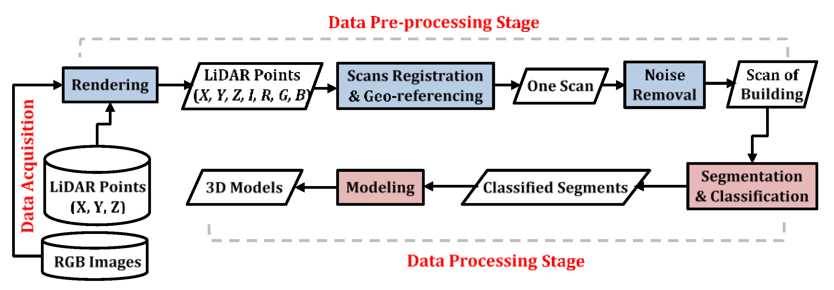
Several researchers have proposed a framework for scan-to-BIM using terrestrial laser scanning (TLS) systems [3,9]. The typical workflow for the scan-to-BIM can be summarized into three main stages: data acquisition stage, data pre-processing stage, and data processing stage as shown in Figure 1. The data acquisition stage includes the determination of a specific level of details of the model required for the BIM application so that the data quality parameters (e.g., accuracy, spatial resolution and coverage) can be identified [3,12]. Data quality is directly associated with scanning device selection and scanning locations. The data pre-processing stage includes data registration, geo-referencing, and de-noising (i.e., noise removal). Most of the previous studies have used commercial software packages for registration, geo-referencing, or noise removal, such as Leica Cyclone [13], Faro Scene [7,14], Trimble Realworks [5] and Autodesk ReCap [7,9,15]. A critical step in data pre-processing is data downsampling or downsizing [10,13,14,16]. Before processing, it is necessary to reduce the massive amount of data, and hence reduce the execution time. For instance, Wang et al. [10] reduced the data by about half its size, while Abdelazeem et al. [15] reduced the data by up to 95%. This was attributed to the method used in data downsampling. The data processing stage includes object recognition from point clouds and modelling those objects as BIM products. Several studies have imported the point clouds directly into commercial software packages for modelling different objects [9]. Others have exported the point clouds after data pre-processing into BIM formats without applying any segmentation methods or object recognition steps using Autodesk Ecotect Analysis [10,17,18], Trimble RealWorks [5] or Autodesk Revit [7,13].

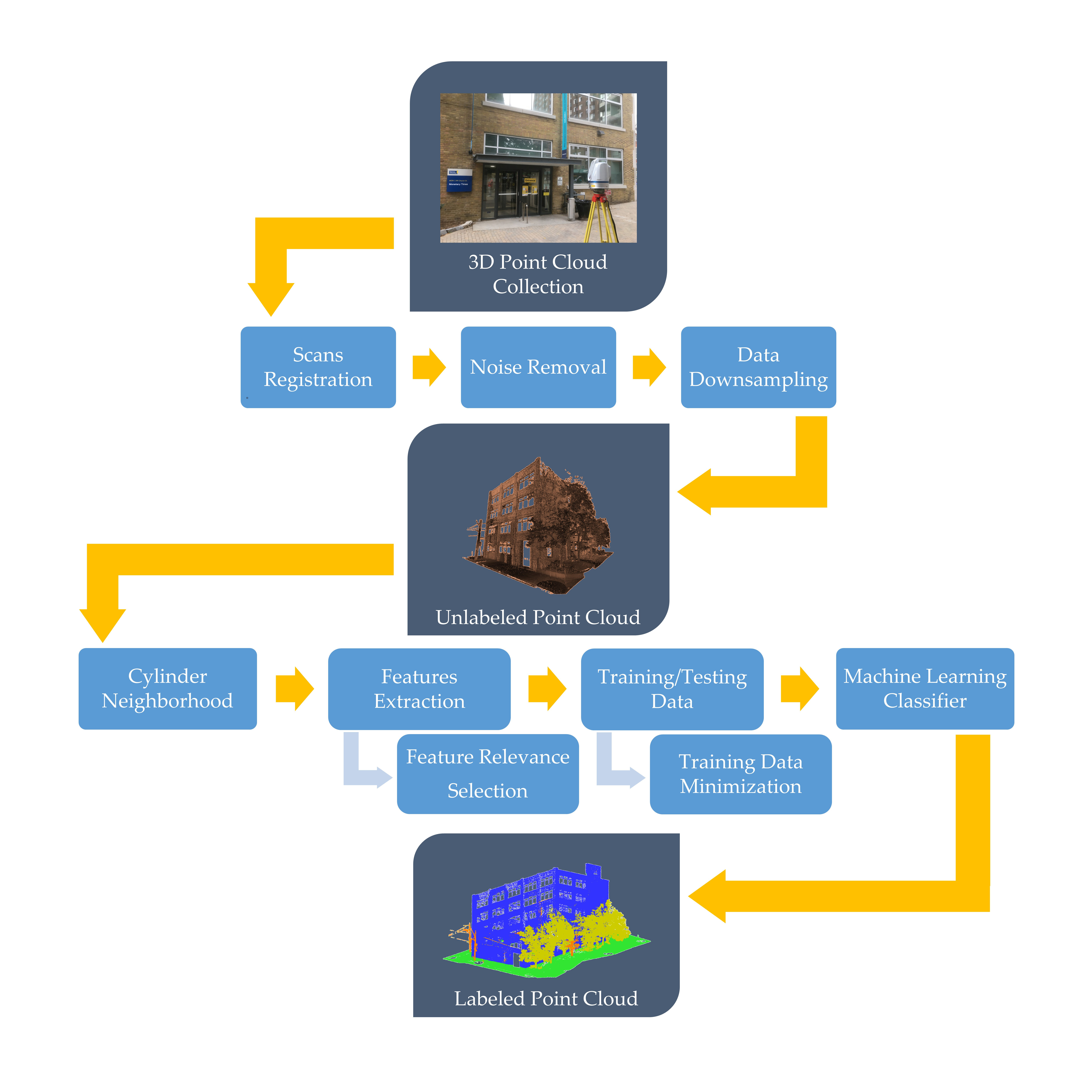
Overall, the scan-to-BIM framework relies on data acquisition, LiDAR point cloud classification, and 3D model construction. In this research, we focus on the LiDAR data classification of existing buildings, which is divided into three steps; neighborhood definition, LiDAR features extraction, and machine learning (ML) algorithms being applied to label each LiDAR point [19,20,21,22]. Generally, the classification results vary according to the implementation of the three aforementioned steps. In addition, the processing time is a crucial factor in LiDAR point cloud classification due to the vast amount of data being collected.

ML algorithms have been widely used in LiDAR data classification. They rely on a pre-trained model on a given data consisting of inputs and their corresponding outputs of the same characteristics. ML-based methods are divided into supervised and unsupervised methods. Supervised methods use attributes [23] or feature descriptors [24] extracted from LiDAR point cloud as inputs to ML algorithms, such as support vector machine (SVM) or random forests (RF) [25,26,27]. Unsupervised methods are based on LiDAR point cloud clustering, such as k-means, DBSCAN (Density-Based Spatial Clustering of Applications with Noise) or hierarchical clustering [28,29,30]. Several studies have used supervised methods, while few have been reported using unsupervised methods. Recent studies have moved to apply deep learning (DL) for point cloud classification, such as neural networks [8,24,31,32,33]. In general, supervised ML and DL-based methods achieve accurate results. However, they require a considerable amount of pre-labeled data to be used in the training process, which is costly and time consuming.

Grilli et al. [25] extracted different LiDAR point features based on the spherical neighborhood selection method. In addition, the Z-coordinate of points were incorporated for accuracy improvement. Then, the features were used as input for the RF classifier. They tested four heritage sites with different features configurations. The average accuracy measures reached 95.14% precision, 96.84% recall, and 95.82% F1-score in the best case studied. Teruggi et al. [27] presented a multi-level and multi-resolution workflow for point cloud classification of historical buildings using RF classifier. They aimed to document detailed objects by applying three levels of searching radius on three levels of point resolution with an average F1-score of 95.83%.

Few studies were reported on building classification from TLS data. Chen et al. [34] adapted the large density variation in the TLS data by presenting a building classification method using density of projected points filter. First, facade points were detected based on a polar grid, followed by applying a threshold to distinguish facades from other objects. The filtering result was then refined using an object-oriented decision tree. The roof points were finally extracted by region growing being applied on the non-facade points. Two datasets were tested in this study and revealed an average completeness and correctness of 91.00% and 97.15%, respectively. Yuan et al. [35] used TLS data for building materials classification using ML algorithms. They evaluated different supervised learning classifiers using material reflectance, color values, and surface roughness. The highest overall accuracy of 96.65% was achieved for classifying ten building materials using the bootstrap aggregated decision trees.

Earlier in the last decade, Martinez et al. [36] proposed an approach for building facade extraction from unstructured TLS point cloud. The main plane of the building’s façade was first extracted using the random sample consensus algorithm (RANSAC) algorithm, followed by establishing a threshold in order to automatically remove points outside the façade. The facade points were then segmented using local maxima and minima in the profile distribution function and statistical layer grouping. Each segmented layer was afterwards processed to find the façade contours. A total of 45 distances were manually measured using a total station as a reference. The mean error was 7 mm, with a standard deviation of 19 mm at an average point spacing of 10 mm. Although the high scores were revealed, the aforementioned approaches were applied on the whole point cloud available, resulting in more processing time and complex computations. Gonzalez et al. [37] used TLS intensity data for damage recognition of historical buildings. Two-dimensional intensity images were generated from the 3D point cloud. Then, three unsupervised classifiers were applied, k-means, ISODATA, and fuzzy k-means, demonstrating average overall accuracy of 75.23%, 60.29%, and 79.85%, respectively. The aforementioned studies relied on either the intensity data [35,37] or the direct use of XYZ coordinates [34,37]. The intensity data require extensive correction and/or normalization that rely on the scan angle and distances between the TLS and scanned objects. On the other hand, geometry-based features are currently extracted from the XYZ coordinates that improve classification accuracies.

Recently, the classification process has been carried out using ML algorithms for BIM applications. In contrast, labeled data are used to train an ML model, and hence that model is used to classify the whole unlabeled dataset. Therefore, high classification accuracy methods running at acceptable processing time are required, especially with the availability of many features that could be extracted from the LiDAR point cloud. The objectives of this paper are as follows: (1) assess the relevance of LiDAR-derived features to 3D point classification, (2) optimize the training data size for LiDAR point cloud classification based on a ML algorithm, and (3) evaluate different scenarios for ML inputs based on the contribution of LiDAR-derived features of the classification process.

2. Materials and Methods

2.1. Methodology

The LiDAR points’ classification method presented in this research is divided into two main phases, data pre-processing and data processing, as shown in Figure 2. Data pre-processing phase starts with noise points’ removal from each scan. Then, multiple scan registration is carried out using bundle adjustment. It uses as many iterative closest points as possible to connect each scan with all its neighbors to globally register the whole dataset [38]. Data downsampling is an essential step in LiDAR data processing either for indoor or outdoor applications. Ground-based laser scanning systems acquire huge amount of data. Thus, a reliable downsampling method is required in order to reduce the processing time. In this research, the space method is used for downsampling the data. It considers a minimum point spacing to preserve the geometry of the building [15,39].

The data processing phase starts with the cylindrical neighborhood selection method, with a predefined radius r. The main challenge here is to find a sufficient number of neighborhood points N for each LiDAR point P, and hence assign each LiDAR point P to its correct class. Previous studies have investigated three common neighborhood methods, namely, K-nearest neighbor (KNN), spherical and cylindrical methods [40,41,42,43]. The KNN neighborhood selection method assigns a predefined number of k nearest points to a query point P of the LiDAR data using the Euclidean distance. Spherical and cylindrical neighborhood methods use a predefined radius r to search neighbor points of a query point P within a sphere or in 2D projection, respectively.

The selection of neighborhood method relies mainly on the point density of the dataset. Searching of neighbors within a fixed radius is usually suitable in a dataset with uniform point density (i.e., our case). Although the cylindrical method gathers the largest number of neighbor points among the three methods its superiority has been proven, especially with using RF classifier [44]. Therefore, neighborhood points are selected based on the cylindrical method in this research, especially with the high capabilities of workstations that are currently available and their ability to process a massive amount of data, and thanks to the downsampling step that decreases the number of points. After that, a total of sixteen LiDAR point features are extracted based on the data geometry (i.e., coordinates). These features are divided into three categories: eight covariance features [40] and verticality (Vert) [45], four moment features [21], and two height features [46], in addition to normalized height feature (NH), as listed in

Table 1. Covariance, moment, height, and verticality LiDAR point features.

Covariance Features	$L_{\lambda }=\frac{e_1-e_2}{e_1}$
	$P_{\lambda }=\frac{e_2-e_3}{e_1}$
	$S_{\lambda }=\frac{e_3}{e_1}$
	$O_{\lambda }=\sqrt[3]{e_1{e}_2{e}_3}$
	$A_{\lambda }=\frac{e_1-e_3}{e_1}$
	$E_{\lambda }=-{\displaystyle {\displaystyle \sum }_{i=1}^3}{e}_{i}ln\left(e_i\right)$
	$C_{\lambda }=e_3$
	$Sum={\lambda }_1+{\lambda }_2+{\lambda }_3$
	$Vert=1-\langle \left(0,0,1\right),v_3\rangle$
Moment Features	$M_{11}={\displaystyle {\displaystyle \sum }_{i=1}^N}\langle \left(p_i-p\right),v_1\rangle$
	$M_{12}={\displaystyle {\displaystyle \sum }_{i=1}^N}\langle \left(p_i-p\right),v_2\rangle$
	$M_{21}={\displaystyle {\displaystyle \sum }_{i=1}^N}\langle \left(p_i-p\right),v_1{\rangle }^2$
	$M_{22}={\displaystyle {\displaystyle \sum }_{i=1}^N}\langle \left(p_i-p\right),v_2{\rangle }^2$
Height Features	$dZ=Z_{max}-Z_{min}$
	$StdZ=\sqrt{\frac{{{\displaystyle \sum }}_{i=1}^N{\left(Z_i-Z_{\mu }\right)}^2}{N}}$
	$NH=Z-Z_{ground}$

.

From each point’s neighborhood, a covariance matrix (Cov) is derived as defined in Equation (1) [47]. The eigenvalues (λ₁, λ₂, λ₃) and eigenvectors (ν₁, ν₂, ν₃) are then calculated. The eight covariance features are linearity (L_λ), planarity (P_λ), scattering (S_λ), omnivariance (O_λ), anisotropy (A_λ), eigen entropy (E_λ), change of curvature (C_λ), and sum of eigenvalues (Sum). The first seven covariance features are derived using the normalized eigenvalues, Equation (2), while the sum feature is calculated from the raw eigenvalues [22,39]. The moment features are 1st order moment around 1st axis (M₁₁), 1st order moment around 2nd axis (M₁₂), 2nd order moment around 1st axis (M₂₁), and 2nd order moment around first axis (M₂₂). The moment features measure the distribution of the cylinder’s points relative to an axis, namely the first and second order moments of the point’s neighborhood around the Eigenvectors ν₁ and ν₂. They help in identifying crease edges and occlusion boundaries [21]. The height features, which include maximum elevation difference (dZ) and standard deviation of elevations (StdZ), are derived from the Z-coordinates within the neighborhood. In addition, the NH feature is defined in this research, which is the height of each point above ground. The Z_ground in this research is defined as the minimum Z-coordinate within the neighborhood of each point. Those sixteen LiDAR-derived features are then used as input for the RF classifier.

$$\mathrm{Cov}=\frac{1}{N}{\displaystyle \sum }_{i=1}^N(p_i-\overline{p}){(p_i-\overline{p})}^T$$

(1)

$$e_{\mathrm{j}}=\frac{{\lambda }_{\mathrm{j}}}{{{\displaystyle \sum }}_{j=1}^3{\lambda }_{\mathrm{j}}}$$

(2)

where:

N = number of points within the neighborhood

p_i = coordinates array of point i

$\overline{p}$ = mean coordinates array

λ_j = eigenvalue

e_j = normalized eigenvalue

The RF algorithm was first proposed by [48]. The RF classifier depends on multiple decision trees in which each decision tree provides a vote to assign each class to an input vector [49]. This type of classification is implemented in two steps, the first is to create learners and then combine the outputs to achieve a good learning algorithm [49]. RF algorithm has proven its capability for point cloud classification and provides acceptable and successful results [43,44]. Therefore, it is applied in this research to separate the building’s points into four classes: ground, facades, trees, and others. A certain percentage of randomly stratified training samples are used to train the model, while the testing step is conducted on the whole dataset to estimate the classification accuracy. This is because we need to label each single point in the dataset to be ready for different applications. In addition, stratified samples are used to ensure the balance in the classes rather than using a fixed number of points for each class (i.e., 1000) that was utilized in previous studies, regardless of the size of each class with respect to the whole dataset [20,21,42]. Finally, the results are evaluated using accuracy metrics, including overall accuracy, precision, recall, and F1-score. For simplicity, the following equations are based on binary classification, which can be extended to the four classes considered in this research.

$$\mathrm{OA}=\frac{\mathrm{TP}+\mathrm{TN}}{\mathrm{TP}+\mathrm{FP}+\mathrm{FN}+\mathrm{TN}}$$

(3)

$$\mathrm{Precesion}=\frac{\mathrm{TP}}{\mathrm{TP}+\mathrm{FP}}$$

(4)

$$\mathrm{Recall}=\frac{\mathrm{TP}}{\mathrm{TP}+\mathrm{FN}}$$

(5)

$$\mathrm{F}1-\mathrm{score}=\frac{2\left(\mathrm{Precision}\ast \mathrm{Recall}\right)}{\left(\mathrm{Precision}+\mathrm{Recall}\right)}$$

(6)

where true positive (TP), false positive (FP), true negative (TN), and false negative (FN) represents the number of correctly identified class, number of incorrectly identified class, number of correctly rejected class, and number of incorrectly rejected class, respectively.

2.2. Study Area and Dataset

The study area is the Monetary Times (MON) building, located at 43°39′35″N 79°22′41″W in Toronto, Canada. The MON building was built by the Municipal Printing Company of Canada in 1931. This building was renovated in the 1980s and became the home school of the Department of Civil Engineering at Toronto Metropolitan University. It is a mid-rise educational building with dimensions of about 33 m by 17 m, which consists of four levels, including offices, classrooms, and laboratories.

We followed the recommendations related to data acquisition mentioned by [50,51]. The scan stations’ positions were chosen to acquire the whole environment without causing redundant data and ensure sufficient overlapping areas between point cloud [50]. We also performed a loop to improve the quality of point cloud registration [51]. A total of ten scans for the building’s outdoor environment were acquired by the Polaris TLS system, manufactured by Teledyne Optech. The specifications of the Polaris system are illustrated in

Table 2. Polaris system specifications.

Parameter	Specification
Range measurement principle	Pulsed
Wavelength	1550 nm (invisible)
Sample collection rate	Up to 2 MHz
Intensity recording	12 bits
Minimum range	1.5 m
Number of returns recorded	Up to 4
Angular resolution	up to 12 μrad
Max. sample density [point to point spacing]	2 mm @ 100 m
Range accuracy (1 sigma)	5 mm @ 100 m
Range resolution	2 mm *
Precision, single shot (1 sigma)	4 mm @ 100 m
Angular accuracy	80 μrad
Max. field of view (vertical)	120° (−45 to +70°)
Max. field of view (hz)	360°
Internal camera resolution	80-Mpix panoramic image

* Min distance that the Polaris is able to separate two range measurements on objects in a similar bearing.

. The scanner’s locations were distributed around the building with at least 50% overlap between scans to ensure accurate scans registration, Figure 3. The configurations of the scanning environment were set as follows: horizontal and vertical field of view was 360° and 120°, respectively; range mode was up to 750 m, and the pulse repetition frequency was 200 kHz with scan frequency of 14.3 Hz. This resulted in each scan lasting for about 6 min and 40 s. Figure 4 shows the data acquired for the MON building, with more than 52 million points.

3. Results and Discussion

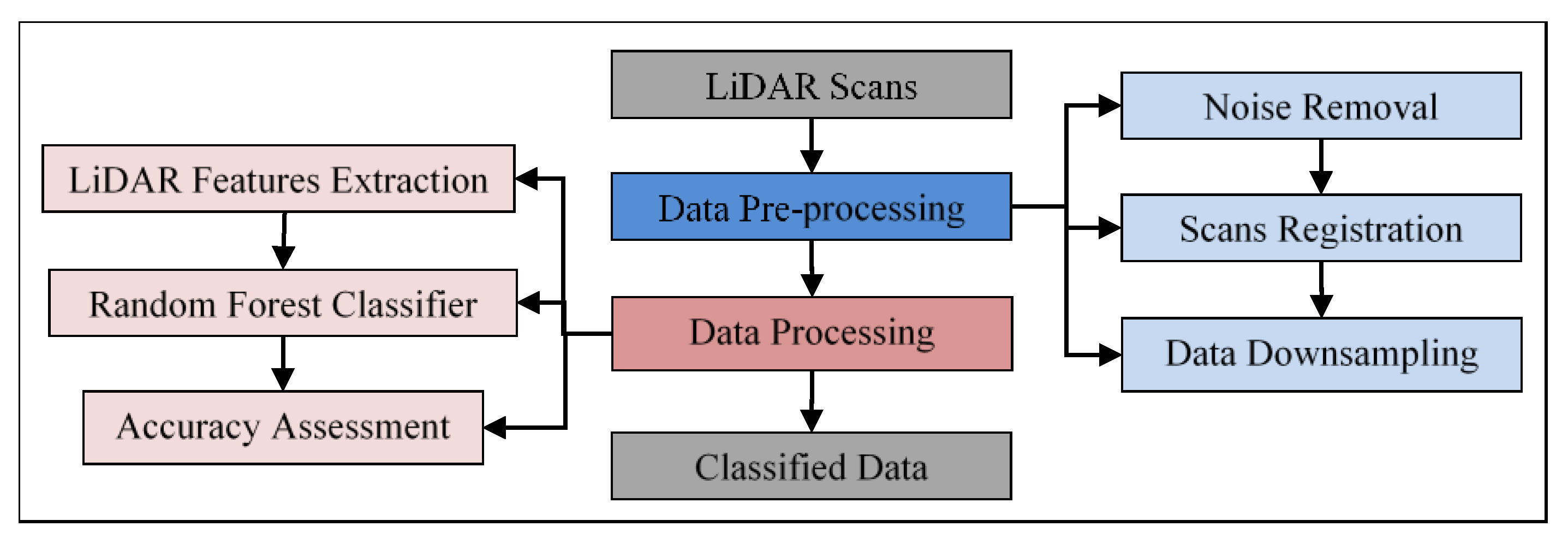
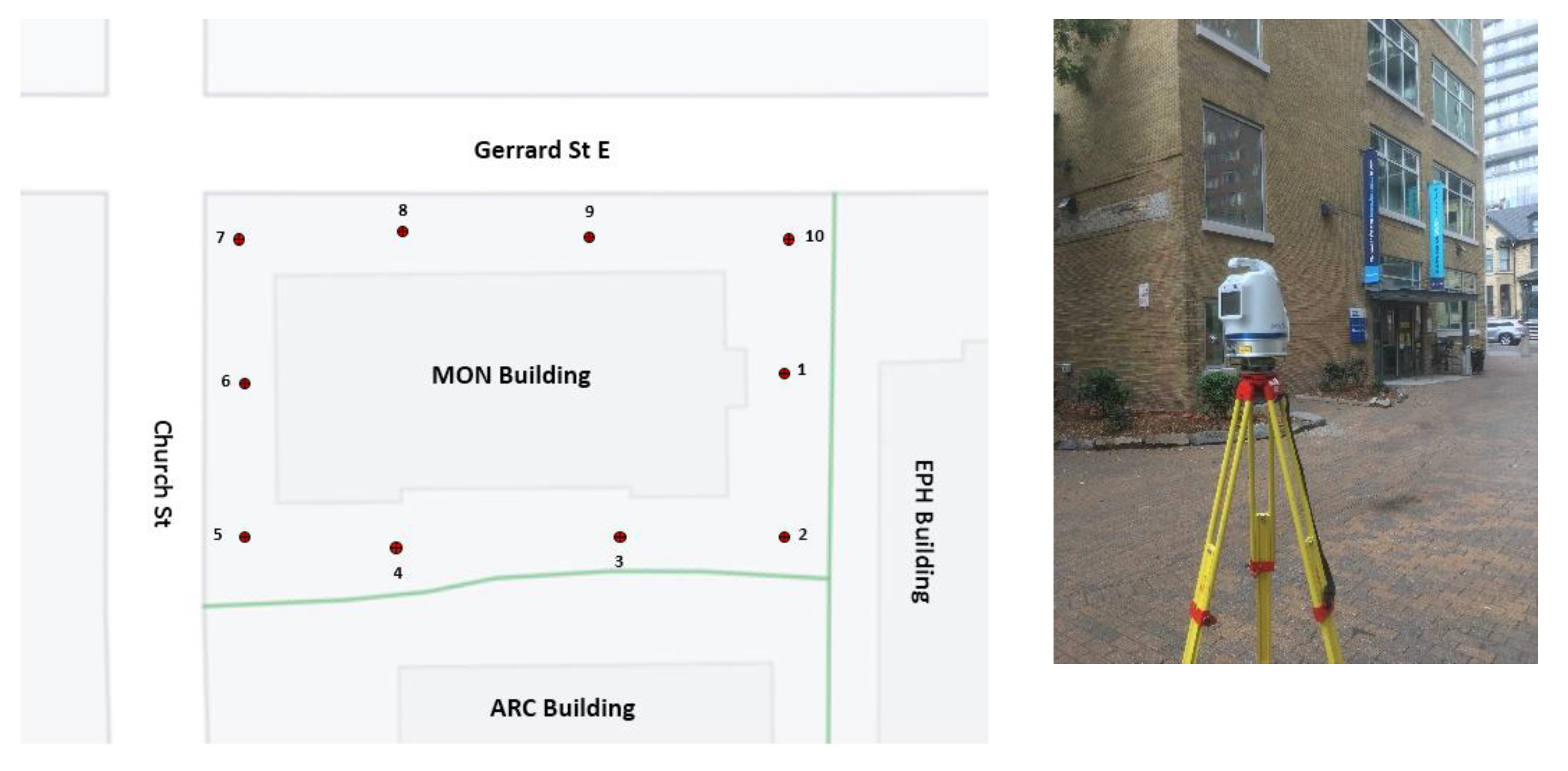
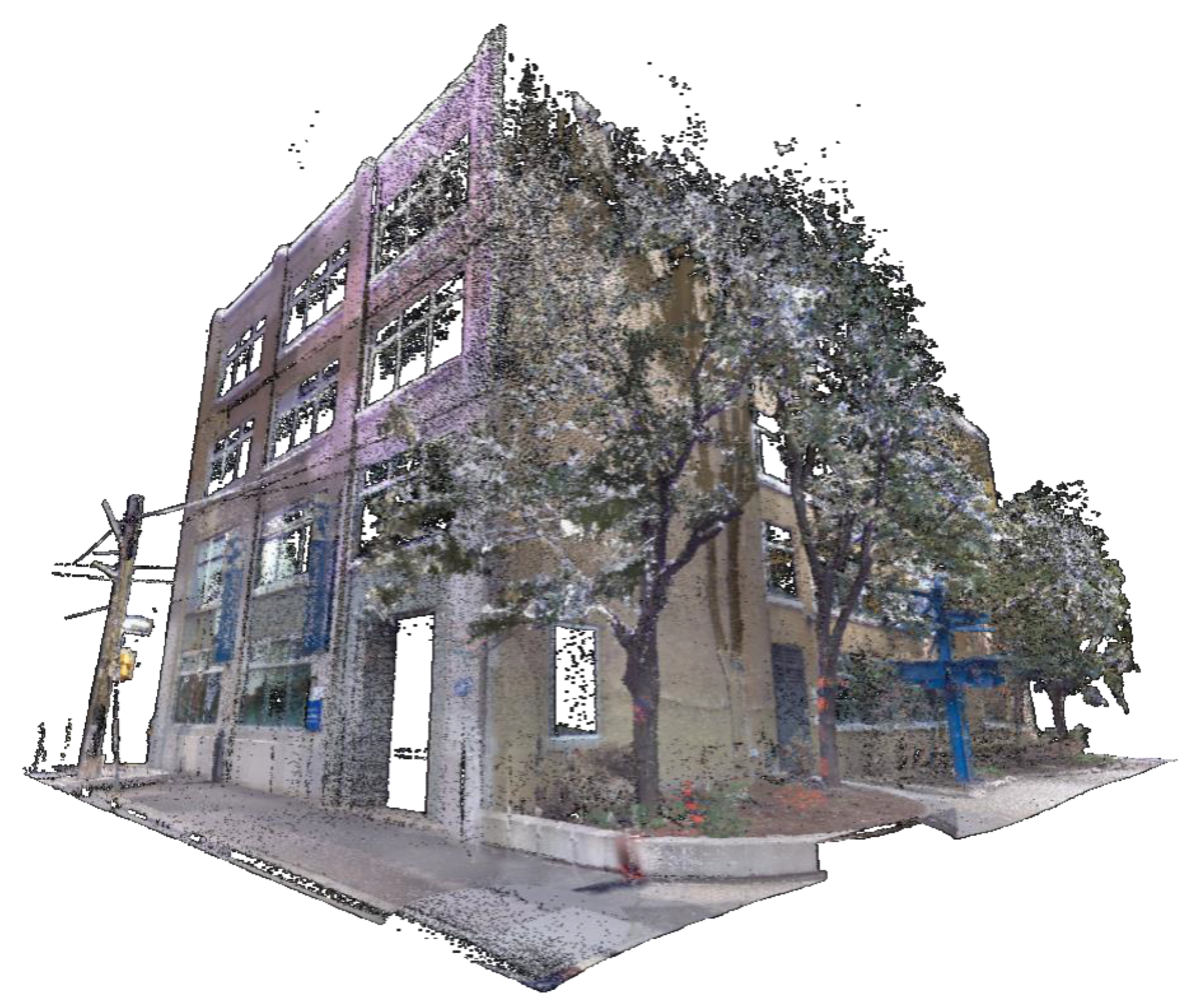
LiDAR point cloud pre-processing was employed using ATLAScan software package, developed by Teledyne Optech for processing Polaris system’s data. First, noise points were removed from each scan. Second, point cloud preregistration step was conducted. The preregistration procedures started by finding three couples of corresponding points among the scans. Then, a rough alignment between the imported scans was employed. Further, a bundle adjustment was carried out to improve the registration accuracy. The average registration error of corresponding points was 0.008 m. Finally, the 3D model for the MON building was created, and the LiDAR data in the format of XYZ were exported with more than 52 million points as shown in Figure 4. It should be noted that the intensity as well as RGB values for each point have not been utilized in this research.

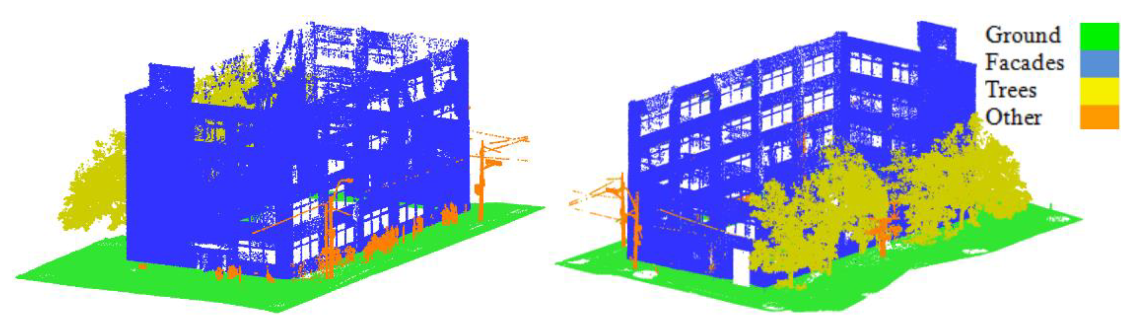
After that, the data were downsampled using the space method function embedded in the CloudCompare software with a point spacing of 2.5 cm to preserve the geometry of the building. Thus, the number of points was decreased by about 95% (about 2.6 million points). Several tests were conducted in order to conclude the suitable point spacing which achieved the desired results without losing the 3D geometry of the data. Point spacing of 0.5, 1.0, 1.5, 2.0, 2.5, 3.0, and 3.5 cm were tested. It was found that the 2.5 cm reduced the number of points and kept the geometry of the building. This was a necessary step in LiDAR point cloud processing to reduce the execution time of either features extraction or points classification. Before proceeding with the data processing phase, the LiDAR points were manually labeled into four classes, namely ground, facades, trees, and others, as shown in Figure 5, to be used in the training/testing process.

Table 3. Total number of points for each class.

Class	Number of Points
Ground	1,330,952
Facades	818,922
Trees	384,469
Others	70,843

provides the number of points for each class.

The data processing phase started with a neighborhood selection method. The cylindrical neighborhood was used with a radius of 0.1 m. This value was a trade-off to ensure a sufficient number of points in the neighborhood and reduce the execution time. Then, the aforementioned sixteen LiDAR geometrical features were extracted to feed the RF classifier. For each point, a 3 × 3 covariance matrix from its neighborhood was derived as shown in Equation (1). Eigenvalues and Eigenvectors were then calculated from the covariance matrix. The eight covariance features, four moment features as well as the Vert feature were extracted. Likewise, the height features were extracted based on the Z-coordinate. The RF classifier was then applied with Gini as the splitting function and hyper-parameters of number of trees equals to 50 and tree depth equals to 50. The training data were selected as randomly stratified to guarantee all classes were presented proportionally to their size in the training data, while the testing step was conducted on the whole dataset. A 10-fold cross-validation was then applied on the training data to evaluate the RF model and resulted in a mean score of 99.18%, with a standard deviation of ±0.02%.

The testing data was evaluated to address the three objectives of this research. First, the sixteen features were considered in the classification process to demonstrate the contribution of each feature. Second, the training data was reduced and the classification accuracy was recorded in order to track the minimal training data used without significant decrease in the accuracy. Third, the impact of using most contributing features to the classification process was studied. The accuracy metrics were finally calculated for the aforementioned cases. The data processing stage was implemented in the Python programing language and run on a Dell machine with Intel^® Xeon^® processor E5-2667 v4, 3.20 GHz and 128 GB RAM.

3.1. Relevance of LiDAR-Derived Features to 3D Point Classification

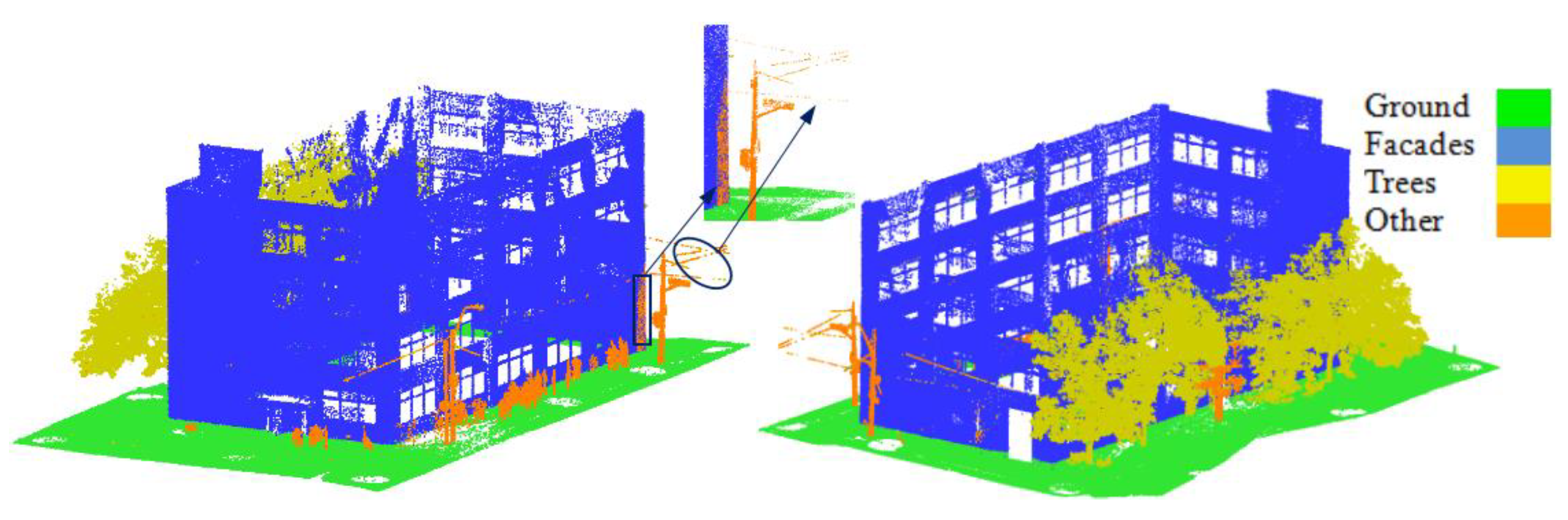
The sixteen LiDAR-derived features were used to classify the dataset. In this case, the training data were used as 50% to demonstrate the capability of each feature. Figure 6 shows the classified point cloud, and

Table 4. Confusion matrix and accuracy metrics of classification results.

Reference	Classification					Recall (%)	F1-Score (%)
	Ground	Façade	Trees	Others	Sum
Ground	1,312,979	524	440	301	1,314,244	99.90	99.89
Façade	715	810,590	1017	6483	818,805	99.00	99.41
Trees	685	298	382,598	828	384,409	99.53	99.44
Others	232	614	1011	68,910	70,767	97.38	93.57
Sum	1,314,611	812,026	385,066	76,522	2,588,225
Precision (%)	99.88	99.82	99.36	90.05

shows the confusion matrix and accuracy metrics of the classification. The results revealed an overall classification accuracy of 99.49%. The accuracy metrics showed high scores for the individual classes.

With the focus on the individual classes, ground, facades, and trees demonstrated more than 99% in all accuracy metrics. On the other hand, the others class demonstrated lower values in accuracy metrics of 90.05%, 97.38% and 93.5% in precision, recall, and F1-score, respectively. This was mainly because this class included many objects, such as streetlights, power lines, road signs, pedestrians, and a small steel structure. This could be because road signs are a planar surface similar to facades and very close to them as shown in Figure 6 (black bounds). About 8.47% of façades points were wrongly classified as others, decreasing the precision of the class. Also, about 1.43% of the others class points were wrongly classified as trees due to the similarity of scatter behavior between and sparse point of power lines.

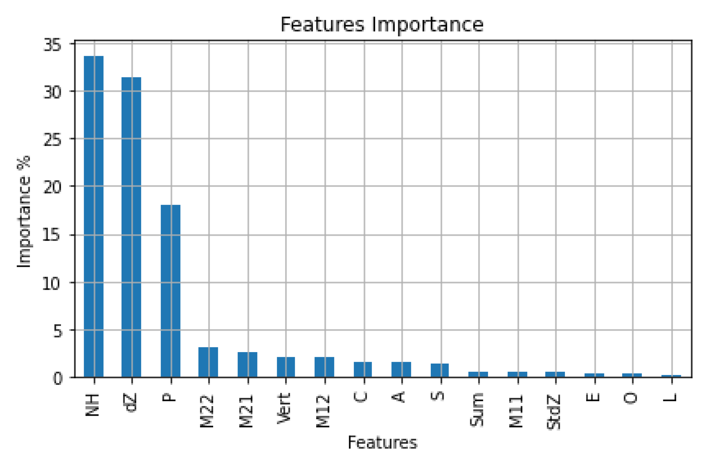
The contribution of LiDAR-derived features to the classification process was then studied. The features importance was calculated as shown in Figure 7. The NH feature was the most contributing feature with 33.55%, while the dZ feature occupied the second order with 31.29%. They were followed by P_λ feature (17.96%), then M₂₂, M_21, Vert, and M₁₂ features, with more than 2% each, while the rest demonstrated less than a 2% contribution. The first three features (i.e., NH, dZ, and P_λ, respectively) were the more significant features in the classification due to the vertically organized LiDAR point cloud of facades and tree trunks as well as facades and ground exhibited planar surfaces.

3.2. Minimal Training Data Determination

In this section, we evaluated the classification accuracy vs. different training data sizes. The purpose of that was to minimize the training data as possible, which in turn reduced the processing time, while maintaining the accuracies at a certain level. Thus, training data of 70%, 50%, 30%, 10%, and 5% were considered with testing the whole dataset. The results of the aforementioned cases are listed in

Table 5. Comparison of different sizes of training dataset. Bold values are close to 99% overall accuracy.

Training	Time (s)	OA %	Avg. Prec. %	Avg. Rec. %	Avg. F1-Score %
70%	372	99.58	97.37	99.30	98.28
50%	259	99.49	97.28	98.95	98.08
30%	150	99.35	97.12	98.42	97.74
10%	45	99.03	96.72	97.03	96.88
5%	21	98.79	96.46	95.91	96.17

.

The results demonstrated that we can reduce the taring data along with preserving the accuracy level. Considering the overall accuracy, we can see a slight decrease from using 70% to 50% training by only 0.09% as well as from using 50% to 30% training by 0.14%, while a significant drop appeared moving to 10% and 5% training by 0.32% and 0.24%, respectively. Thus, 99% overall accuracy could be achieved with using 10% training data, with reduction of processing time reaching about 88% (70% training data) and 83% (50% training data). It should be noted that the presented time in Table 4 is only for training and testing process. The features extraction time was about 90 min for the sixteen features. In addition, the low time (i.e., in seconds) of training and testing process was due to the high capability of the workstation used. 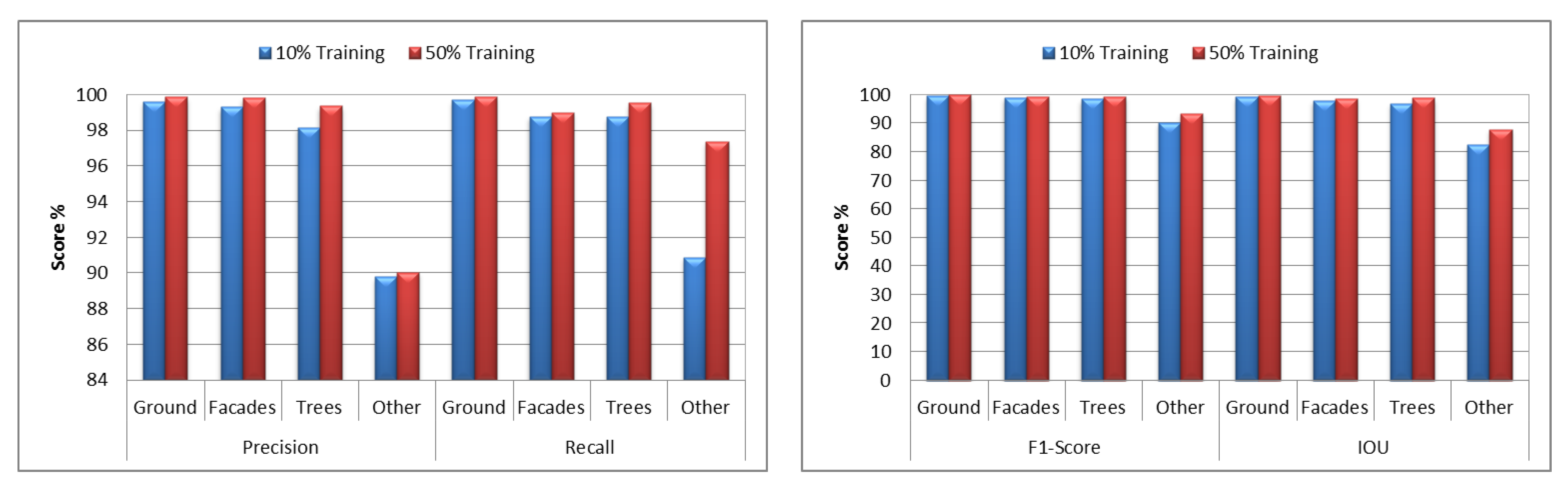Figure 8 shows the individual classes’ accuracy measures of 10% and 50% training data. Ground, facades, and trees classes have close accuracy metrics for both training cases, while the others class from 10% training data has lower accuracy metrics than those from 50% training data. However, this is acceptable as the main classes have achieved high accuracy metrics.

3.3. The Impact of Features Reduction

Section 3.1 demonstrated the order of features that contributed to the classification process. In this section, the six most relevant features (i.e., NH, dZ, P_λ, M22, M21, and Vert) as well as three features (i.e., NH, dZ, and P_λ) were studied in terms of accuracy metrics and processing time. The features extraction time for the six and three features were about 66 min and 47 min, respectively, with a decrease of extraction time by 27% and 48% compared to sixteen features extraction.

Table 6. Comparison of different sizes of training dataset using six features (NH, dZ, P_λ, M22, M21, Vert). Bold values are close to 99% overall accuracy.

Training	Time (s)	OA %	Avg. Prec. %	Avg. Rec. %	Avg. F1-Score %
70%	108	99.57	97.40	99.22	98.27
50%	73	99.46	97.28	98.81	98.02
30%	38	99.30	97.09	98.13	97.59
10%	10	98.92	96.65	96.58	96.61
5%	5	98.60	96.07	95.43	95.74

and

Table 7. Comparison of different sizes of training dataset using three features (NH, dZ, P_λ). Bold values are close to 99% overall accuracy.

Training	Time (s)	OA %	Avg. Prec. %	Avg. Rec. %	Avg. F1-Score %
70%	47	99.42	97.37	98.44	97.89
50%	31	99.14	96.61	97.67	97.12
30%	16	98.85	96.24	96.43	96.33
10%	5	98.19	95.05	94.43	94.73
5%	3	97.83	94.50	93.24	93.84

provide the accuracy metrics and processing time against different sizes of training data for testing six and three features, respectively.

Considering the most important six features, the training and classification time reduced from 45 s to 10 s, by about 78%. The use of 10% training data achieved the overall accuracy level at 99%. To preserve 99% overall accuracy using the three features with the highest importance, a 50% training set should be considered. The training and classification time were decreased by about 31% in this case.

3.4. Comparison with Previous Studies

The literature is lacking studies concerned about the minimization of training data of point cloud classification. On the other hand, many studies considered LiDAR data classification using different LiDAR-derived features, different neighborhood selection, and different classification methods [19,20,21,40,42,46]. Those studies demonstrated classification accuracies between 85.70% and 97.55%, while our method achieved a higher score of 99% average overall accuracy. It should be noted that we only considered four classes (ground, facades, trees, and others).

For a quantitative comparison, we applied the proposed LiDAR-derived features in previous studies on our dataset. For instance, Weinmann et al. [20] tested twelve 3D features, including the eight covariance features, verticality, the two height features, and point density. They also tested 2D features, but we focused here on the features extracted from 3D points directly. Among different features sets, Weinmann et al. [40] evaluated the eight covariance features only as eigenvalue-based features. Hackel et al. [21] added four moment features and two height features defined as height below and height above the tested points, but excluded the height standard deviation (dZ). As a result, they tested sixteen LiDAR-derived features.

Table 8. F1-score (%) and OA (%) comparison with previous studies. Highest values are bolded.

Class	3D Features [20]	Eigenvalue-Based Features [40]	Hackel Features [21]	Ours
Ground	98.70	86.87	98.76	99.89
Façade	95.41	72.70	95.36	99.41
Trees	93.24	85.45	93.00	99.44
Others	81.42	50.00	81.69	93.57
Average F1-score	92.19	73.75	92.20	98.08
OA	96.41	81.12	96.40	99.49

provides F1-score and overall accuracy of the aforementioned studies compared to our case. It is shown that we have achieved high scores of F1-score for all individual classes and overall accuracy. Thus, the achieved classification results have proven the usefulness of incorporating the NH feature.

4. Conclusions

In this paper, we have classified the 3D point cloud of a campus building using LiDAR geometrical features and an RF classifier. The NH, a LiDAR-derived feature had the highest contribution percentage (more than 30%) to the classification process. The overall classification accuracy was improved by about 4.16% when the NH feature was incorporated. In addition, precision, recall and F1-score have been improved for all classes.

Supervised ML classifiers, such as the RF classifier, in most cases, achieve good results. However, they require a massive amount of annotated dataset to be used as training samples. Therefore, in this research, we tested different training data sizes against the overall accuracy and execution time. Using 10% of the whole dataset as training samples has demonstrated about 99% overall accuracy with 82% reduction of training and classification time compared to using 50% training samples.

Since the execution time is crucial in the classification process, we have tested a reduced number of features for the classification. The six and three most relevant features to the classification process were evaluated. A significant drop of features extraction time was achieved by about 27% and 48% compared to sixteen features extraction time. Also, the training and classification time was decreased by about 78% and 40%, respectively, to preserve the overall classification accuracy at 99%. Overall, this paper gives a variety of options for using training data to achieve certain accuracies with acceptable processing time.

Improvement of point cloud classification is the first step toward digital model creation that is expected to help in making informed decisions about existing buildings, such as designing of a reconstruction or extension, improvement of the building’s energy efficiency, and implementation of a smart campus or city. It also opens doors for BIM-related applications, such as the operation and maintenance, heritage documentation, and structural health monitoring. Future work will focus on incorporating the intensity and RGB values collected with the data and test their ability in improving the results of 3D point cloud classification. In addition, high-detailed building elements and building indoor environment, as well as infrastructure-related applications such as road/railways maintenance, and bridges inspection will be considered.

References

1. Ma, Z.; Ren, Y. Integrated application of BIM and GIS: An overview. Procedia Eng. 2017, 196, 1072–1079. [Google Scholar] [CrossRef]
2. The 2nd Annual BIM Report. 2019. Available online: https://buildinginnovation.utoronto.ca/reports/ (accessed on 28 January 2022).
3. Wang, Q.; Guo, J.; Kim, M.K. An application oriented scan-to-BIM framework. Remote Sens. 2019, 11, 365. [Google Scholar] [CrossRef] [Green Version]
4. Liu, J.; Xu, D.; Hyyppa, J.; Liang, Y. A survey of applications with combined BIM and 3D laser scanning in the life cycle of buildings. IEEE J. Sel. Top. Appl. Earth Obs. Remote Sens. 2021, 14, 5627–5637. [Google Scholar] [CrossRef]
5. Almukhtar, A.; Saeed, Z.O.; Abanda, H.; Tah, J.H. Reality capture of buildings using 3D laser scanners. CivilEng 2021, 2, 214–235. [Google Scholar] [CrossRef]
6. Aziz, M.A.; Idris, K.M.; Majid, Z.; Ariff, M.F.M.; Yusoff, A.R.; Luh, L.C.; Abbas, M.A.; Chong, A.K. A study about terrestrial laser scanning for reconstruction of precast concrete to support QCLASSIC assessment. ISPRS Arch. Photogramm. Remote Sens. Spat. Inf. Sci. 2016, 42, 135–140. [Google Scholar] [CrossRef] [Green Version]
7. Rocha, G.; Mateus, L.; Fernández, J.; Ferreira, V. A scan-to-BIM methodology applied to heritage buildings. Heritage 2020, 3, 47–67. [Google Scholar] [CrossRef] [Green Version]
8. Matrone, F.; Grilli, E.; Martini, M.; Paolanti, M.; Pierdicca, R.; Remondino, F. Comparing machine and deep learning methods for large 3D heritage semantic segmentation. ISPRS Int. J. Geo-Inf. 2020, 9, 535. [Google Scholar] [CrossRef]
9. Badenko, V.; Fedotov, A.; Zotov, D.; Lytkin, S.; Volgin, D.; Garg, R.D.; Min, L. Scan-to-BIM methodology adapted for different application. ISPRS Arch. Photogramm. Remote Sens. Spat. Inf. Sci. 2019, 42, 1–7. [Google Scholar] [CrossRef] [Green Version]
10. Wang, C.; Cho, Y.K.; Kim, C. Automatic BIM component extraction from point clouds of existing buildings for sustainability applications. Automat. Constr. 2015, 56, 1–13. [Google Scholar] [CrossRef]
11. Ward, Y.; Morsy, S.; El-Shazly, A. GIS-BIM data integration towards a smart campus. In Proceedings of the Joint International Conference on Design and Construction of Smart City Components, Cairo, Egypt, 17–19 December 2019; pp. 132–139. [Google Scholar]
12. Dai, F.; Rashidi, A.; Brilakis, I.; Vela, P. Comparison of image-based and time-of-flight-based technologies for three-dimensional reconstruction of infrastructure. J. Constr. Eng. M 2013, 139, 69–79. [Google Scholar] [CrossRef]
13. Jung, J.; Hong, S.; Jeong, S.; Kim, S.; Cho, H.; Hong, S.; Heo, J. Productive modeling for development of as-Built BIM of existing indoor structures. Automat. Constr. 2014, 42, 68–77. [Google Scholar] [CrossRef]
14. Macher, H.; Landes, T.; Grussenmeyer, P. Point clouds segmentation as base for as-Built BIM creation. ISPRS Ann. Photogramm. Remote Sens. Spat. Inf. Sci. 2015, 2, 191. [Google Scholar] [CrossRef] [Green Version]
15. Abdelazeem, M.; Elamin, A.; Afifi, A.; El-Rabbany, A. Multi-sensor point cloud data fusion for precise 3D mapping. Egypt. J. Remote Sens. Sp. Sci. 2021, 24, 835–844. [Google Scholar] [CrossRef]
16. Wu, K.; Shi, W.; Ahmed, W. Structural elements detection and reconstruction (SEDR): A hybrid approach for modeling complex indoor structures. ISPRS Int. J. Geo-Inf. 2020, 9, 760. [Google Scholar] [CrossRef]
17. Wang, C.; Cho, Y. Automated 3D building envelope recognition from point clouds for energy analysis. In Proceedings of the Construction Research Congress, West Lafayette, IN, USA, 21–23 May 2012; pp. 1155–1164. [Google Scholar]
18. Wang, C.; Cho, Y.K. Performance evaluation of automatically generated BIM from laser scanner data for sustainability analyses. Procedia Eng. 2015, 118, 918–925. [Google Scholar] [CrossRef] [Green Version]
19. Chehata, N.; Guo, L.; Mallet, C. Airborne LiDAR feature selection for urban classification using random forests. ISPRS Arch. Photogramm. Remote Sens. Spat. Inf. Sci. 2009, 38, W8. [Google Scholar]
20. Weinmann, M.; Jutzi, B.; Hinz, S.; Mallet, C. Semantic point cloud interpretation based on optimal neighborhoods, relevant features and efficient classifiers. ISPRS J. Photogramm. Remote Sens. 2015, 105, 286–304. [Google Scholar] [CrossRef]
21. Hackel, T.; Wegner, J.D.; Schindler, K. Fast semantic segmentation of 3D point clouds with strongly varying density. ISPRS Ann. Photogramm. Remote Sens. Spat. Inf. Sci. 2016, III-3, 177–184. [Google Scholar] [CrossRef] [Green Version]
22. Mohamed, M.; Morsy, S.; El-Shazly, A. Improvement of 3D LiDAR point cloud classification of urban road environment based on random forest classifier. Geocarto Int. 2022, 1–23. [Google Scholar] [CrossRef]
23. Nguyen, A.; Le, B. 3D point cloud segmentation: A survey. In Proceedings of the 6th IEEE Conference on Robotics, Automation and Mechatronics (RAM), Manila, Philippines, 12–15 November 2013; pp. 225–230. [Google Scholar]
24. Chen, J.; Kira, Z.; Cho, Y.K. Deep learning approach to point cloud scene understanding for automated scan to 3D reconstruction. J. Comput. Civil. Eng. 2019, 33, 04019027. [Google Scholar] [CrossRef]
25. Grilli, E.; Farella, E.M.; Torresani, A.; Remondino, F. Geometric feature analysis for the classification of cultural heritage point clouds. In Proceedings of the 27th CIPA International Symposium, Ávila, Spain, 1–5 September 2019; pp. 541–548. [Google Scholar]
26. Grilli, E.; Remondino, F. Machine learning generalisation across different 3D architectural heritage. ISPRS Int. J. Geo-Inf. 2020, 9, 379. [Google Scholar] [CrossRef]
27. Teruggi, S.; Grilli, E.; Russo, M.; Fassi, F.; Remondino, F. A hierarchical machine learning approach for multi-level and multi-resolution 3D point cloud classification. Remote Sens. 2020, 12, 2598. [Google Scholar] [CrossRef]
28. Lu, X.; Yao, J.; Tu, J.; Li, K.; Li, L.; Liu, Y. Pairwise linkage for point cloud segmentation. ISPRS Ann. Photogramm. Remote Sens. Spat. Inf. Sci. 2016, III-3, 201–208. [Google Scholar]
29. Poux, F.; Mattes, C.; Kobbelt, L. Unsupervised segmentation of indoor 3D point cloud: Application to object-based classification. ISPRS Arch. Photogramm. Remote Sens. Spat. Inf. Sci. 2020, 44, 111–118. [Google Scholar] [CrossRef]
30. Grilli, E.; Poux, F.; Remondino, F. Unsupervised object-based clustering in support of supervised point-based 3D point cloud classification. ISPRS Arch. Photogramm. Remote Sens. Spat. Inf. Sci. 2021, 43, 471–478. [Google Scholar] [CrossRef]
31. Qi, C.R.; Su, H.; Mo, K.; Guibas, L.J. Pointnet: Deep learning on point sets for 3D classification and segmentation. In Proceedings of the IEEE Conference on Computer Vision and Pattern Recognition, Honolulu, HI, USA, 21–26 July 2017; pp. 652–660. [Google Scholar]
32. Qi, C.R.; Yi, L.; Su, H.; Guibas, L.J. Pointnet++: Deep hierarchical feature learning on point sets in a metric space. In Proceedings of the 31st Conference on Neural Information Processing Systems (NIPS), Long Beach, CA, USA, 4–9 December 2017; pp. 1–10. [Google Scholar]
33. Pierdicca, R.; Paolanti, M.; Matrone, F.; Martini, M.; Morbidoni, C.; Malinverni, E.S.; Frontoni, E.; Lingua, A.M. Point cloud semantic segmentation using a deep learning framework for cultural heritage. Remote Sens. 2020, 12, 1005. [Google Scholar] [CrossRef] [Green Version]
34. Chen, M.; Liu, X.; Zhang, X.; Wang, M.; Zhao, L. Building extraction from terrestrial laser scanning data with density of projected points on polar grid and adaptive threshold. Remote Sens. 2021, 13, 4392. [Google Scholar] [CrossRef]
35. Yuan, L.; Guo, J.; Wang, Q. Automatic classification of common building materials from 3D terrestrial laser scan data. Automat. Constr. 2020, 110, 103017. [Google Scholar] [CrossRef]
36. Martínez, J.; Soria-Medina, A.; Arias, P.; Buffara-Antunes, A.F. Automatic processing of terrestrial laser scanning data of building façades. Automat. Constr. 2012, 22, 298–305. [Google Scholar] [CrossRef]
37. Armesto-González, J.; Riveiro-Rodríguez, B.; González-Aguilera, D.; Rivas-Brea, M.T. Terrestrial laser scanning intensity data applied to damage detection for historical buildings. J. Archaeol. Sci. 2010, 37, 3037–3047. [Google Scholar] [CrossRef]
38. Optech ATLAScan Help. 2019. Available online: https://www.scribd.com/document/526409308/ATLAScan-Help (accessed on 28 January 2022).
39. Mohamed, M.; Morsy, S.; El-Shazly, A. Evaluation of data subsampling and neighbourhood selection for mobile LiDAR data classification. Egypt. J. Remote Sens. Sp. Sci. 2021, 24, 799–804. [Google Scholar] [CrossRef]
40. Weinmann, M.; Jutzi, B.; Mallet, C. Semantic 3D scene interpretation: A framework combining optimal neighborhood size selection with relevant features. ISPRS Ann. Photogramm. Remote Sens. Spat. Inf. Sci. 2014, 2, 181. [Google Scholar] [CrossRef]
41. Blomley, R.; Jutzi, B.; Weinmann, M. Classification of airborne laser scanning data using geometric multi-scale features and different neighbourhood types. ISPRS Ann. Photogramm. Remote Sens. Spat. Inf. Sci. 2016, III-3, 169–176. [Google Scholar] [CrossRef] [Green Version]
42. Thomas, H.; Goulette, F.; Deschaud, J.E.; Marcotegui, B.; LeGall, Y. Semantic classification of 3D point clouds with multiscale spherical neighborhoods. In Proceedings of the 6th International Conference on 3D Vision (3DV), Verona, Italy, 5–8 September 2018; pp. 390–398. [Google Scholar]
43. Mohamed, M.; Morsy, S.; El-Shazly, A. Machine learning for mobile LiDAR data classification of 3D road environment. ISPRS Arch. Photogramm. Remote Sens. Spat. Inf. Sci. 2021, 44, 113–117. [Google Scholar] [CrossRef]
44. Mohamed, M.; Morsy, S.; El-Shazly, A. Evaluation of machine learning classifiers for 3D mobile LiDAR point cloud classification using different neighborhood search methods. Adv. LiDAR 2022, 2, 1–9. [Google Scholar]
45. Demantk’e, J.; Vallet, B.; Paparoditis, N. Streamed vertical rectangle detection in terrestrial laser scans for façade database production. ISPRS Ann. Photogramm. Remote Sens. Spatial Inf. Sci. 2012, I-3, 99–104. [Google Scholar] [CrossRef] [Green Version]
46. Weinmann, M.; Jutzi, B.; Mallet, C. Feature relevance assessment for the semantic interpretation of 3D point cloud data. ISPRS Ann. Photogramm. Remote Sens. Spatial Inf. Sci. 2013, III-5/W2, 313–318. [Google Scholar] [CrossRef] [Green Version]
47. Jutzi, B.; Gross, H. Nearest neighbour classification on laser point clouds to gain object structures from buildings. ISPRS. Arch. Photogramm. Remote Sens. Spat. Inf. Sci. 2009, 38, 4–7. [Google Scholar]
48. Breiman, L. Random forests. Mach. Learn. 2001, 45, 5–32. [Google Scholar] [CrossRef] [Green Version]
49. Pino-Mejías, R.; Cubiles-de-la-Vega, M.D.; Anaya-Romero, M.; Pascual-Acosta, A.; Jordán-López, A.; Bellinfante-Crocci, N. Predicting the potential habitat of oaks with data mining models and the R system. Environ. Model. Softw. 2010, 25, 826–836. [Google Scholar] [CrossRef]
50. Wang, Q.; Sohn, H.; Cheng, J.C. Automatic As-built BIM Creation of Precast Concrete Bridge Deck Panels Using Laser Scan Data. J. Comput. Civ. Eng. 2018, 32, 04018011. [Google Scholar] [CrossRef]
51. Macher, H.; Landes, T.; Grussenmeyer, P. From point clouds to building information models: 3D semi-automatic reconstruction of indoors of existing buildings. Appl. Sci. 2017, 7, 1030. [Google Scholar] [CrossRef]
Figure 1. Typical scan-to-BIM workflow. The data pre-processing stage is in blue color and the data processing stage is in magenta color.
Remotesensing 14 05934 g001
Figure 2. LiDAR point cloud classification workflow. The workflow input (3D point cloud) and output (classified point cloud) are in gray color, the data pre-processing stage is in blue color and the data processing stage is in magenta color.
Remotesensing 14 05934 g002
Figure 3. Scans’ locations (from 1 to 10) around the MON building (left) and the Polaris system scanning the building from Station #2 (right).
Remotesensing 14 05934 g003
Figure 4. MON building 3D model.
Remotesensing 14 05934 g004
Figure 5. Different views of the labeled LiDAR point cloud of the building.
Remotesensing 14 05934 g005
Figure 6. Classified point cloud using sixteen features with classification errors in black bounds.
Remotesensing 14 05934 g006
Figure 7. Features importance for of the sixteen features.
Remotesensing 14 05934 g007
Figure 8. Precession, Recall, and F1-score from for 10% and 50% training.
Remotesensing 14 05934 g008