Article

Plant Density Estimation Using UAV Imagery and Deep Learning

1
Key Laboratory of Ecosystem Network Observation and Modeling, Institute of Geographic Sciences and Natural Resources Research, Chinese Academy of Sciences, Beijing 100101, China
2
University of Chinese Academy of Sciences, Beijing 100190, China
3
Shandong Dongying Institute of Geographic Sciences, Institute of Geographic Sciences and Natural Resources Research, Chinese Academy of Sciences, Dongying 257000, China
4
Leibniz Centre for Agricultural Landscape Research (ZALF), 15374 Müncheberg, Germany
5
Department of Crop Sciences, University of Göttingen, Von-Siebold-Str. 8, 37075 Göttingen, Germany
6
Key Laboratory of Land Surface Pattern and Simulation, Institute of Geographic Sciences and Natural Resources Research, Chinese Academy of Sciences, Beijing 100101, China
7
State Key Laboratory of Resources and Environmental Information System, Institute of Geographic Sciences and Natural Resources Research, Chinese Academy of Sciences, Beijing 100101, China
8
CAS Engineering Laboratory for Yellow River Delta Modern Agriculture, Institute of Geographic Sciences and Natural Resources Research, CAS, Beijing 100101, China
9
Yusense Information Technology and Equipment (Qingdao) Inc., Qingdao 266000, China
*
Author to whom correspondence should be addressed.
Remote Sens. 2022, 14(23), 5923; https://doi.org/10.3390/rs14235923
Submission received: 20 September 2022 / Revised: 11 November 2022 / Accepted: 17 November 2022 / Published: 23 November 2022
(This article belongs to the Special Issue Machine Learning Methods Applied to Optical Satellite Images)

Abstract

:
Plant density is a significant variable in crop growth. Plant density estimation by combining unmanned aerial vehicles (UAVs) and deep learning algorithms is a well-established procedure. However, flight companies for wheat density estimation are typically executed at early development stages. Further exploration is required to estimate the wheat plant density after the tillering stage, which is crucial to the following growth stages. This study proposed a plant density estimation model, DeNet, for highly accurate wheat plant density estimation after tillering. The validation results presented that (1) the DeNet with global-scale attention is superior in plant density estimation, outperforming the typical deep learning models of SegNet and U-Net; (2) the sigma value at 16 is optimal to generate heatmaps for the plant density estimation model; (3) the normalized inverse distance weighted technique is robust to assembling heatmaps. The model test on field-sampled datasets revealed that the model was feasible to estimate the plant density in the field, wherein a higher density level or lower zenith angle would degrade the model performance. This study demonstrates the potential of deep learning algorithms to capture plant density from high-resolution UAV imageries for wheat plants including tillers.

1. Introduction

Plant density is a critical variable for crop growth and yield by influencing inter- and intraspecific competition for the available resources (e.g., water, nutrients, and radiation) [1]. During the growth season, sowing and planting densities should be similar in optimal conditions. However, poor emergence, competition for resources, extreme weather events, technical issues within sowing machinery, and pests and diseases would influence planting density over the growing period [2,3,4,5]. Moreover, plant arrangements in the field are pivotal to precise crop management, which can determine plant establishment and growth [2,3] and guide site-specific irrigation and fertilization [6,7]. Therefore, developing accurate, detailed, and non-destructive approaches for plant density monitoring is crucial.
Plant density monitoring was traditionally based on ground counts within quadrats or segments [2]. Manually counting plants in the field is time-consuming and destructive, making it impossible to undertake over a large area. Remote sensing, which typically observes crops from a canopy top view, can monitor plant density over extended areas [8]. According to platforms, remote sensing can be categorized into three main types: satellite, proximal, and unmanned aerial vehicle (UAV) [9]. Observing crops from space, satellite remote sensing can estimate extensive plant distribution by employing empirical relationships between ground measurements and vegetation indices [10]. However, satellite-based sensors have limitations in presenting details, especially for identifying field-scale individual plants due to coarse spatial resolutions [8]. The proximal platform can provide high-resolution images for plant counting, which has been widely used for plant density surveys [2,11,12]. However, its application in practice is either impeded by large observing frame installation (e.g., gantry-based platforms) or limited with flexibility in field panoramic observation (e.g., handheld, pole-based, or unmanned ground vehicle-based platforms). Benefiting from significant progress in hardware and decreased equipment cost, unmanned aircraft vehicles (UAVs) have become a promising platform for conducting plant density surveys [9]. Moreover, it is feasible to acquire high-resolution images of individual plants using UAVs due to their flexibility in flight altitude [13].
However, pinpointing single plants from dense canopies within UAV images (e.g., more than 1000 plants per image in this study) is still challenging. Although manually counting plants from UAV imagery is relatively simple and straightforward, exploring big imagery data from multiple UAV campaigns is labor-intensive and time-consuming [14]. In order to resolve this challenge, various automatic techniques have been proposed to estimate plant density from UAV images [15,16,17]. Pixel-based classification methods, such as threshold setting and supervised regression, are the least complex and most commonly used methods for counting plants in the imageries [18,19,20,21]. These methods are adequate for segmenting plant pixels but have limited accuracy in plant counting [22]. Machine learning has been proposed to distinguish plant instances in remote sensing imagery to improve model performance in plant counting [13,23]. However, the performance of the machine learning algorithms is often limited in complex conditions (e.g., overlay existing among plants), mainly because machine-learning-based identifying is still based on pixel-based classification.
Recent advances in deep learning, an artificial intelligence subfield, have opened up new possibilities in remote sensing [24]. As a result of deep convolutional networks’ ability to extract image features, deep-learning-based image identification has gathered remarkable results, and computer vision techniques have been constantly updated in order to achieve better results [25]. It has become increasingly common to use deep learning to estimate plant density [12,14,16,26]. A single-stage object detection algorithm (YOLOv3) was adopted for cotton plant detection from low-altitude UAV images [27]. Machefer et al. [28] employed the Mask R-CNN algorithm to realize plant numbers and sizing for potatoes and lettuce in UAV imagery [29]. Additionally, a Faster R-CNN-based pipeline was developed for cotton seedling detection and counting in proximal sensed videos [11]. Therefore, deep learning has proved to be a powerful tool for plant density estimation with robust performance. Nevertheless, these deep learning approaches for plant density estimation mainly depended on bounding box-based object detection, lacking the capacity to monitor dense plants with an overlay to each other on the image.
Generally, the plant density is stable from the preliminary development stage. The plant densities of some row crops (e.g., maize and soybean) from emergence to harvest are essentially constant in optimal growing conditions in the absence of severe biotic and abiotic stressors. On the other hand, some other crops (e.g., wheat, rice and barley) can compensate for low plant densities from emergencies with a tillering mechanism [2]. The previous wheat plant density studies were normally carried out shortly after crop emergence when plants were still present as individuals. For instance, Liu et al. [2] developed an automated wheat seedling count method based on skeleton optimization. An estimation of wheat plant density at the early stage was executed by identifying the green pixels from RGB images [1]. Jin et al. [13] developed a pipeline to estimate wheat plant density at emergence using support-vector-machine-based number counting. These studies accurately captured the plant density at emergence, but the wheat plant density after tillering still needs further exploration. Specifically, unlike wheat plants before tillering, mainly presented as individual plants, the plants after tillering are highly clustered and more challenging to be identified. Nevertheless, wheat plant density including tillers is a crucial variable for following growth stages. Firstly, tillers are a significant supplement to low main-stem density and seedling abortion [30,31]. Secondly, intraspecific competition exists between main stems and tillers for available resources such as light and nutrition [32,33]. Thirdly, tillers can make an important contribution to grain yield, providing partial wheat heads at the mature stage [34].
The objective of this study was to detect the wheat plant density after the tillering stage by leveraging a UAV and deep learning. For this purpose, a deep learning model, DeNet, was developed to generate a heatmap of wheat plant. Then, the wheat counting was derived according to the sum of the heatmap. To validate the performance of DeNet, two typical deep learning algorithms (i.e., SegNet and U-Net) were adopted as benchmarks [35,36]. At the same time, the DeNet was firstly validated on annotation-based images and then tested on field-sampling-based wheat density datasets.

2. Materials and Methods

2.1. Study Area and Data Acquisition

This study’s field works include field sampling and a UAV flight campaign. The field sampling obtained wheat plant numbers in quadrats for testing the accuracy of the plant density model in the field condition. The UAV flight campaign collected images to observe the wheat plant density remotely.

2.1.1. Study Area

The wheat field was located in the yellow river delta (118°55′17.91″N, 37°40′17.94″E) (Figure 1a). This coastal area suffers from salinization (with soil salt content at 3–15 g/kg for 0–20 cm soil depth) as a newly formed river delta (approximately 80 years). The altitude of this flat area is 6 m above sea level. The mean annual temperature of this area is 13.2 °C for the year of 2021, with the maximum and minimum value at 34.7 and −16.1 °C, respectively. The annual precipitation sum of this area is 511 mm for the year of 2021, with most precipitation in summer. The winter wheat (Triticum aestivum L.) field trial sampling site is presented in Figure 1b. The sowing density was 320 seed/m2 with a row interval of 15 cm. In addition, the wheat plants in this area suffered a drought stress in this year with only limited rainfed irrigation (a total of 75 mm precipitation from the sowing day on October 15, 2020 to the field sampling day at March 29, 2021). Thus, wheat plants were under heterogeneous growing status (with distinct plant density) because of dual stresses from salinization and drought.

2.1.2. Field Sampling

From March 29 to 31, 2021, wheat plant counting was conducted at three sampling regions (red boxes in Figure 1b). Three sampling areas (blue boxes in Figure 1b) within sampling regions were dedicatedly selected to make the dataset more comprehensive, covering an increasing gradient of plant density (B < A < C) with marginal effect considered. Ten sampling quadrats with an area of 0.50 m × 0.50 m were set for manual wheat plant counting after the tillering stage at each sampling area (Figure 1c). Main stems and tillers with three or more fully developed leaves were treated as individual plants during the plant counting because tillers with three or more leaves are nutritionally independent of the main stem [37]. As a result, 30 quadrats with plant densities ranging between 45 and 136 plant/plot were recorded.

2.1.3. UAV Flight Campaigns

A DJI Mavic Air 2 UAV (DJI Innovation Company Inc., Shenzhen, China) with a built-in sensor was adopted in the image acquisition from March 27 to 28, 2021, from 11:00 to 13:00 local time, under a sunny weather condition. The UAV system collected orthoimages containing red, green, and blue channels at three meters above ground altitude. The image spatial resolution was 48 MP (8000 × 6000), with the ground sampling distance at approximately 0.4 mm. The UAV flights were divided into two campaigns: with and without a sampling quadrat.
As for the campaign with a sampling quadrat, nine images were obtained for each quadrat (30 quadrats in total). More specifically, these nine images for a quadrat were obtained with the quadrat distributed at nine different locations in the corresponding images (Figure 1d). As for the campaign without a sampling quadrat, images were randomly collected within four flight regions (orange boxes in Figure 1b) without overlay among images. In total, 370 UAV images were collected in the flight campaigns, including 270 images with a sampling quadrat and 100 images without a sampling quadrat (Table 1).

2.2. Image Preparation and Postprocessing

This section introduces how to prepare the full UAV images for inputting into the density estimation model and how to process the model outputs further. These procedures include allocating data into three parts (training, validation, and test), splitting images into image patches (to fit the memory limitations of the graphics card), annotating images for model training and evaluation, and assembling the model-generated heatmaps according to the original sequence.

2.2.1. Image Allocation

Full UAV images were allocated into three parts: training, validation, and test dataset (Table 1). The training and validation datasets did not cover sampling quadrats within the images, whereas the test datasets did. The training set was employed to train the plant density estimation model. The validation set was used to validate the model performance with various configurations in regard to neural network architectures, sigma values, and assembling techniques. The test set was used to test the model performance based on field sampling. The image numbers for training and validation were 85 and 15 to robustly satisfy the model training and validation functions, respectively. Images with the sampling quadrats were allocated to the test dataset. No image was repeatedly included in the three datasets to avoid data corruption.

2.2.2. Image Splitting and Heatmap Assembling

Before the model development, full UAV images were split into image patches to fit the memory capacity of the graphics card. Comprised of multi-layer neural networks, the plant density estimation model would generate a mass of temporary data. These temporary data would be stored in the graphics card for deep learning models that adopted the CUDA (compute unified device architecture) technique to accelerate processing [38]. Generally, the full images would immensely exceed the memory capacity of the graphics card. A standard solution to this problem is splitting the full images into smaller patches [15,39]. Thus, full images in training, validation, and test datasets were split into image patches with different procedures.
As for the training dataset, full images were split into 2550 image patches with the size of 1200 × 1200 pixels (without overlay), while the smaller patches at the image edge were abandoned (Table 1). Regarding the validation dataset, full images were split into 1200 × 1200 pixels’ patches with an overlay between adjacent patches (Figure 2). The overlay ensured that the interested objects (wheat plants) divided by cut-off lines would be integrally presented on the adjacent patches. The overlap width was set to 320 pixels, following the principle that the overlap should be wider than the wheat plant (approximately 150 to 250 pixels on the images). Therefore, each full UAV image was divided into 7 × 9 patches (patches at the image edge may have different sizes). In total, 945 patches were obtained in the validation dataset. As for test datasets with sampling quadrats, the image patch was detached from each full image along the quadrat border. In total, 270 image patches were obtained in the test dataset with the patch height (or width) ranging between 1200 and 1300 pixels.
As for the validation dataset, the plant-density-model-generated heatmaps (with more details in Section 2.3.1) were assembled according to the original sequence of image patches to present the plant density on full images (Figure 2). Two approaches were adopted to fuse the heat value on adjacent heatmaps within the overlay area: the average heat value and the normalized inverse distance weighted (NIDW) heat value. The average heat value was derived by averaging the heat value on overlapped heatmaps, whereas the NIDW heat value was derived as Equation (1).
H e a t i + 1 = ( D o v e r l a y   D b o r d e r ) *   H e a t i + D b o r d e r   *   H e a t p a t c h D o v e r l a y ,
where Heati+1 and Heati are the heatmaps for the (i+1)th and ith assembled images in the irritation, respectively; Heatpatch is the heatmap for image patch; and Dborder and Doverlay (with the unit of the pixel) are the distance to the nearest border of image patch and the width of overlay strip, respectively.

2.2.3. Image Annotation

The ‘labelme’ graphical image annotation tool was employed to draw points on wheat plants (Figure 2) [40]. Annotating the points was a tough task since wheat plants might be clustered after tillering. Accordingly, the annotation task was carried out in two procedures: (i) the annotated point was set on the main stem if the main stem was visible on the image; otherwise, (ii) the annotated point was set on leaves by visually interpreting the wheat plants through the leaf morphology. In order to reduce subjective biases, the annotation task was carried out by two operators, with one charging for drawing points and the other one charging for checking results. Notably, the training and validation datasets were annotated on full images with annotations split together with the image in the splitting operation. In contrast, the test dataset was annotated on image patches after image splitting. The annotation task cost approximately a month for these two operators, with eight hours daily.

2.3. Deep Learning Models

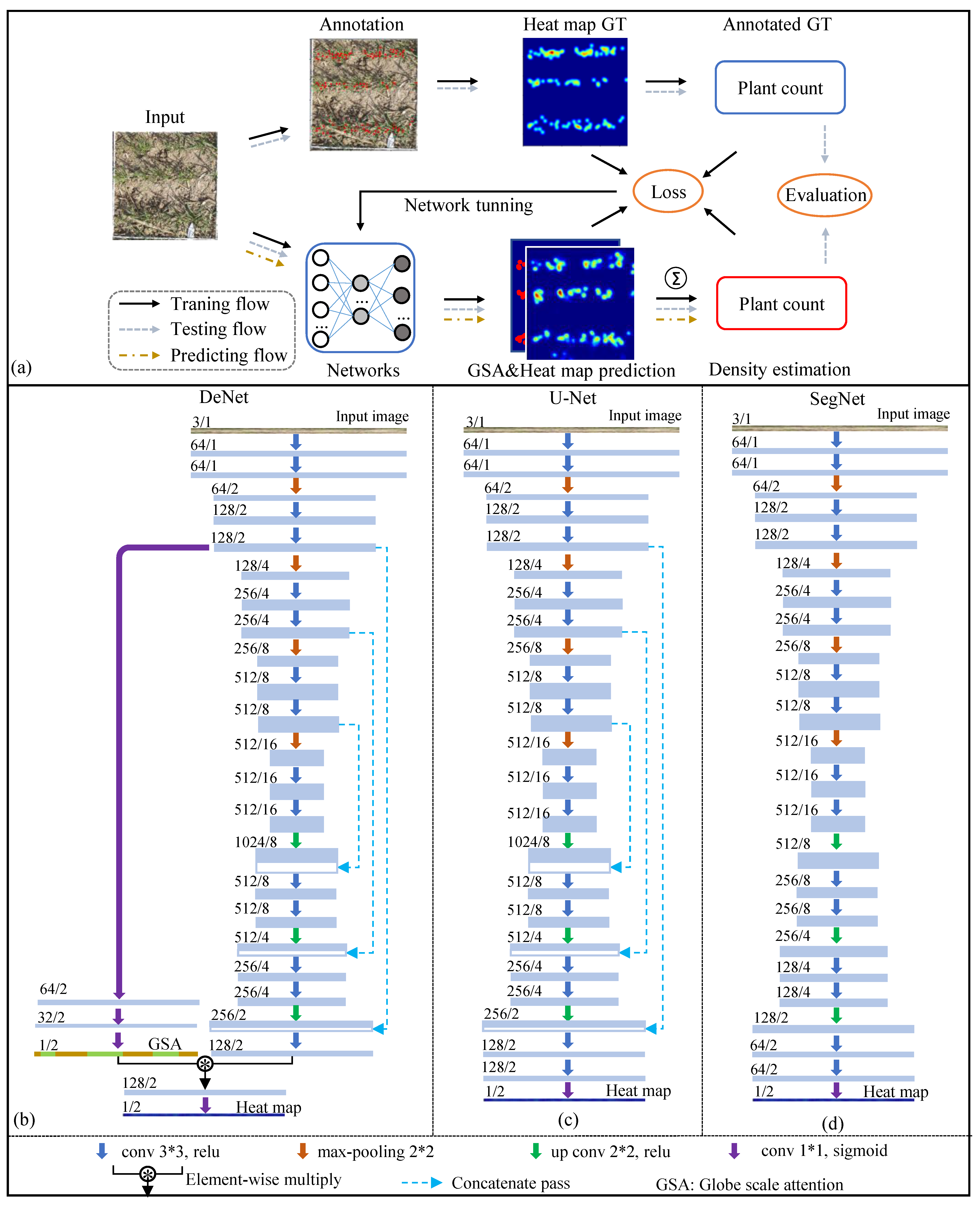
This study developed a Gaussian heatmap-based deep learning model to estimate the wheat plant density in the field. This section introduced five main components of the model, including the network architecture, the gaussian heatmap, the loss function, the evaluation criteria and running environment. The workflow of the plant density estimation model is shown in Figure 3a.

2.3.1. Network Architecture

In this study, we proposed a convolutional neural network (CNN)-based DeNet to estimate the plant density on UAV images. Two classic deep learning networks, the SegNet and the U-Net, were employed as references to compare with DeNet [35,36]. The VGG-13 architecture was adopted as the backbone in the encoding part for three architectures [41]. Specifically, the DeNet could be treated as a successor of SegNet or U-Net with similar architecture (Figure 3b–d). To improve the model performance, we added a global-scale attention branch to the U-Net to compose the DeNet (Figure 3b,c). This branch aims to promote the model’s ability to distinguish wheat plants and backgrounds in a whole image scope, following previous studies that used the global-scale attention to capture an overall distribution of the interested objects [42,43,44]. Specifically, our global-scale attention branch has relatively shallow convolutional layers. It only contained one down-sampling operation (with down-sampling stride = 2), because distinguishing wheat plants from the background (e.g., soil and straw) mainly depended on pixel-level color features. In contrast, deep convolutional neural networks, which mainly focus on spatial features, such as texture and structure features, were not critical in this step [25]. Additionally, this shallow global-scale attention branch would not occupy much computing power in the prediction. In a word, the global-scale attention branch was designed to realize an efficient separation between plant and background using limited computing power.

2.3.2. Gaussian Heatmap

The Gaussian heatmap was adopted to bridge image-scale prediction and plant count. As a common practice in most point-based tasks, heatmaps have been widely applied in deep learning domains, such as human pose estimation, keypoint-based object detection, and crowd counting [45,46,47]. The heatmaps were generated from annotated points with a normalized Gaussian kernel in the following steps. Firstly, the heat value around an annotated point was generated according to the Gaussian distribution within a window size (µ) [Equation (2)]. Then, the heat value in a specific pixel was normalized with the total heat value within the window size [Equation (3)]. Lastly, the heatmap of the specific point was added to the whole heatmap, and other annotated points were iterated with the above steps. Here, the default sigma (σ) value was set at 15, and the window size was set as two times sigma (σ) value for generating heatmaps. Moreover, the plant count of the image patch was obtained by integrating the predicted heatmap after model prediction [Equation (4)].
H e a t = 1 2 π σ e   x 2 + y 2 2   σ 2 ,
H e a t n o r m a l i z e d = H e a t   /   H e a t μ ,
C o u n t = j = 1 h k = 1 w H e a t ( j ,     k ) ,
where sigma (σ) represents the scale parameter of Gaussian distribution; x and y represent widthways and lengthways distances to the specific annotated point, respectively; Heatµ is the heat value for pixels within the window size (µ); h and w represent the height and width of the heatmap, respectively; and Heat (j, k) is the heat value for the specific pixel at (j, k) on the heatmap.

2.3.3. Loss Function

The optimization of the plant density model was based on a loss function consisting of three branches: the heatmap loss (LHM), the global-scale attention loss (LGSA), and the plant count loss (LCT) [Equation (5)]. The heatmap loss adopted the Euclidean loss between heatmaps from ground-truth and prediction [Equation (6)]. The global-scale attention loss adopted the binary cross-entropy between global-scale attention maps from ground-truth and prediction [Equation (7)]. The plant count loss adopted the relative error of plant count between ground-truth and prediction [Equation (8)]. Here, the heatmap loss played a prominent role in model optimization, whereas the global-scale attention loss and plant count loss were axillaries. Notably, the global-scale attention loss was only adopted for the DeNet, but was not feasible for SegNet and U-Net.
L o s s =   L HM + β   L GSA + γ   L C T ,
L HM = 1 2 n   i = 1 n ( x i y i ) 2 ,
L GSA = 1 n i = 1 n [ l i × log p i + ( 1 l i ) × log p i ] ,
L C T = | C P r e C G T | C G T ,
where the α, β, and γ are used to control the relative weights of the three losses with the default value of 1000, 1, and 0.1, respectively; n represents the total pixel number in maps; xi and yi represent heat value on the annotated heatmap and predicted heatmap, respectively; li and pi represent target classes (plant or background) for specific pixels on the annotated heatmap and global-scale-attention-based map, respectively; and CGT and CPre represent plant count from annotation and prediction for each image, respectively.

2.3.4. Evaluation Criteria

Three metrics were adopted to evaluate the plant density estimation results: the coefficient of determination (R2), the mean absolute error (MAE), and the root-mean-squared error (RMSE), as expressed in Equations (9)–(11), respectively, wherein R2 is a non-dimensional value located in [0,1], with a higher value representing the better model performance in plant density estimation. MAE and RMSE had the unit of ‘plant/patch’ or ‘plant/quadrat’ in this study, with the smaller value representing the better model performance in estimation.
R 2 = 1 i = 1 n ( P R i G T i ) 2 i = 1 n ( P R i P R i ¯ ) 2 ,
M A E = i = 1 n | P R i G T i | n ,
R M S E = i = 1 n ( P R i   G T i ) 2 n ,
where n represents the total number of evaluated predictions; PRi and GTi represent the plant count from prediction and ground-truth, respectively.

2.3.5. Running Environment

The experiments were performed on a graphics workstation with an NVIDIA GeForce RTX 3090 graphics card, an Intel Core i9-10920X CPU, and 64 GB memory capacity. The deep learning models were implemented on the deep learning framework Keras [48]. During model training, the Adam algorithm was adopted for network optimization with the learning rate set at 1 × 10⁻⁵ [49].

3. Experiments and Results

3.1. Model Validation

This study proposed a DeNet to estimate wheat plant density. Before the model test on the field-sampling-based dataset, the model was validated with three aspects on the validation dataset. First, the DeNet was compared with the U-Net and SegNet to verify the model performance. Second, a sensitivity analysis was executed on the sigma value for Gaussian heatmap generation to select the optimal value for wheat plant identification. Third, the performance of different image-assembling techniques was validated.

3.1.1. Comparison of Different Networks

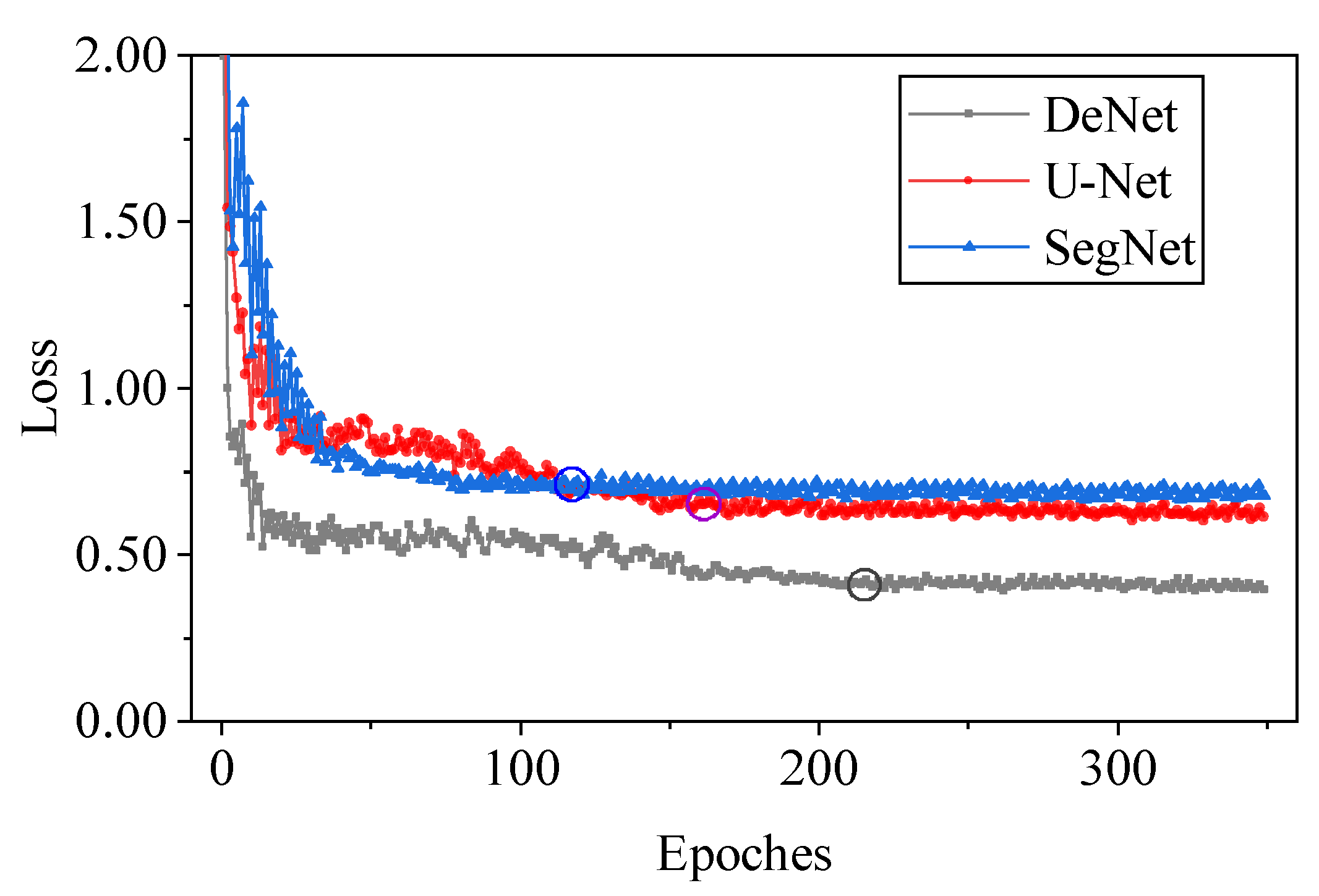
DeNet, U-Net, and SegNet were developed using the training dataset with 350 epochs, respectively (Figure 4). Overall, the three models reached stable convergences. Specifically, the training results indicated that the complexity of networks (from SegNet to U-Net, and then DeNet) could improve loss performance after convergence. However, the convergence time for SegNet, U-Net, and DeNet gradually increased, with convergence appearing at the 130th, 160th, and 220th epochs, respectively. At last, the training time was increased along with the complex model architecture, with a time-cost of 8.8, 9.1, and 9.5 min/epoch for SegNet to U-Net, then DeNet, respectively (Table 2).
The model evaluation on the validation dataset showed that the estimation accuracy was in the order of SegNet < U-Net < DeNet (Table 2). Here, the DeNet obtained the best performance among the three models, indicating that the proposed global-scale attention channel benefited model performance. The outperformance of U-Net over the SegNet proved that the concatenate pass mechanism added in the U-Net (Figure 3c,d) also benefited model performance. Moreover, the predicted heatmaps from the three models were remarkably different (Figure 5). The background area was gradually cleared up, whereas the heated area was gradually agminated from SegNet to U-Net, then DeNet. Such a phenomenon revealed that the global-scale attention was effective in plant and background separation.

3.1.2. Sensitivity Analysis on Sigma

The sigma (σ) was a critical variable for generating the heatmaps of ground-truth [Equation (2)], significantly influencing the model performance in plant density estimation. In this section, a quantitative analysis was carried out to verify the influence of different sigma values on model performance on the validation dataset. The experiments compared models of different sigma values in two rounds with the backbone of DeNet (Table 3). In the first round, a set of integers as multiples of 4 was validated to make a fuzzy diagnosis for the sigma value. In the second round, the integers near the optimal sigma value from the first round were further validated to make a precise diagnosis for the sigma value.
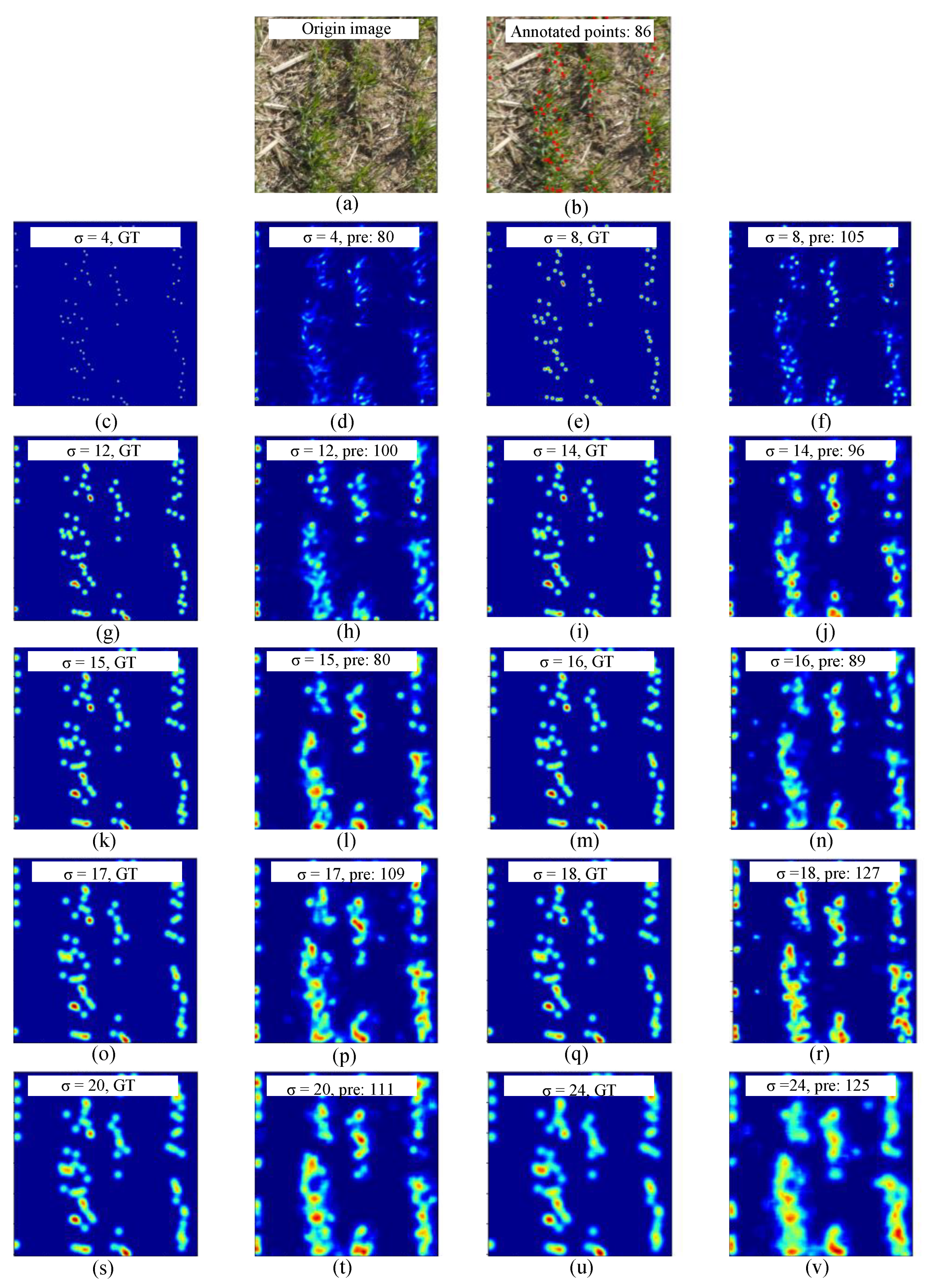
For the first round of sensitivity analysis on the sigma value, the model harvested the best performance when the sigma value was 16 (MAE = 12.11, RMSE = 16.21, R2 = 0.82). As the sigma value increased or decreased from 16, the model performance degraded. In the second round of sensitivity analysis, all models with various sigma values did not surpass the model performance with a sigma value of 16. To sum up, the sensitivity analysis experiment revealed that the sigma value at 16 was the optimal choice for plant density estimation. On the other hand, the predicted heatmaps showed significant differences along with the change in sigma values (Figure 6). Generally, smaller sigma values predicted more centralized heatmaps, while larger ones predicted more fused heatmaps.

3.1.3. Heatmap Assembling

The predicted heatmaps need to be assembled to present the results integrally since the full UAV images were split into image patches before the model execution (as mentioned in Section 2.2.2). The averaging and NIDW techniques were adopted to derive the heat values in the overlapped area. Here, the DeNet and sigma values at 16 were deployed to the plant density model.
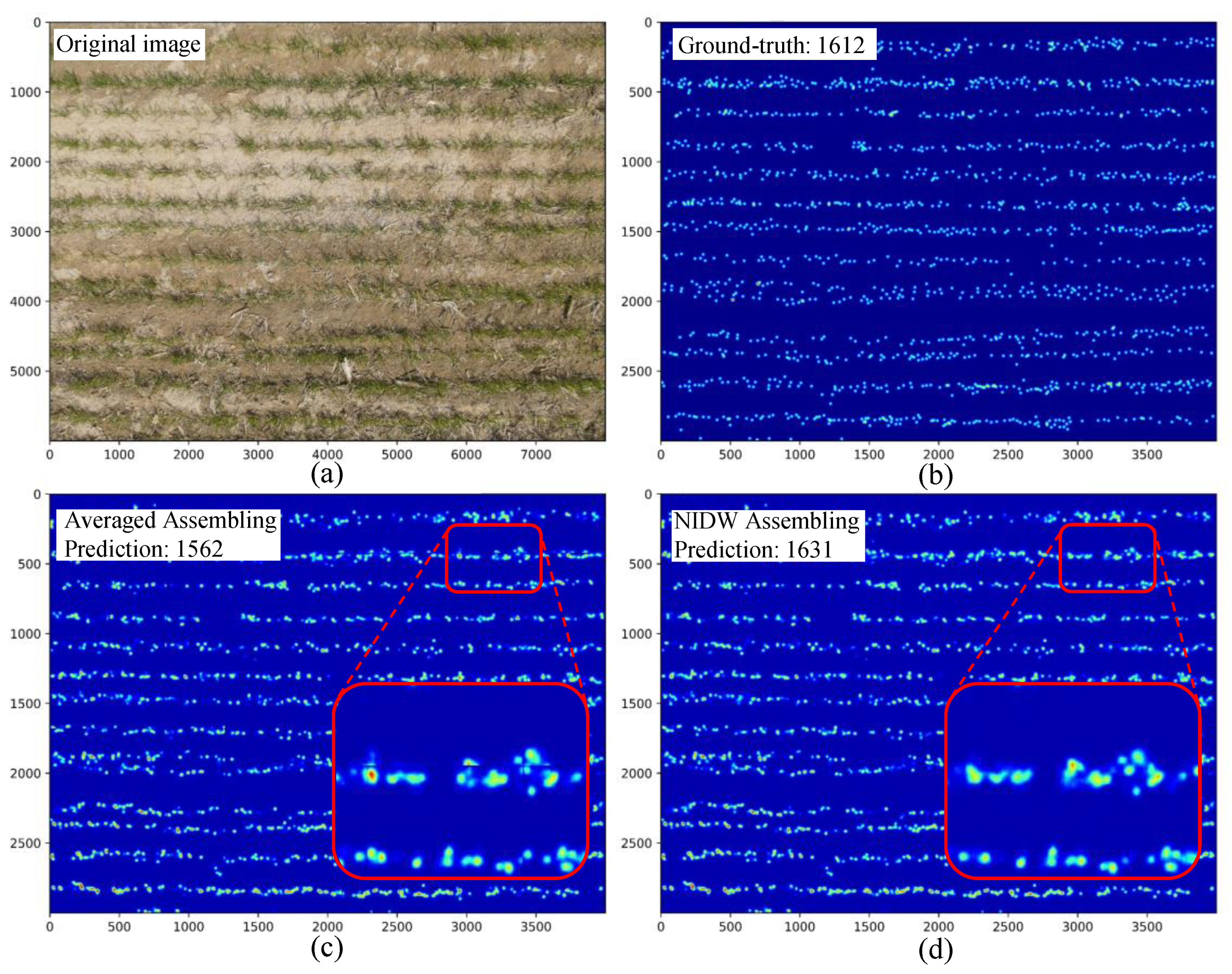
The model prediction results showed that the assembling procedure slightly improved the model performance for both assembling techniques (averaging or NIDW heat value) (Table 4). This phenomenon could be explained by the fact that the overlay area could suppress the errors brought in by padded pixels at the image edge in convolutional operations. Specifically, the NIDW technique performed better than the averaging technique in suppressing this error. Moreover, fissures were easy to find on the assembled heatmaps using the averaging technique when the cut-off line passed through the wheat plants in the image splitting (Figure 7c). However, such issues were handled on the assembled heatmaps using the NIDW technique (Figure 7d).

3.2. Model Test

This section assessed the performance of plant density estimation models using the test dataset. Here, the model predictions were evaluated by two sets of ground-truthing, i.e., the annotation-based and the sampling-based ground-truths. This section deployed a sigma value of 16 and an architecture of DeNet on the plant density models.

3.2.1. Field-Sampling-Based Plant Density Estimation

Comparisons were made among the sampled ground-truth, annotated ground-truth, and predictions using the test dataset (Figure 8). The comparison between sampled ground-truth and annotated ground-truth reached a high consistency, with MAE, RMSE, and R2 values of 7.9, 10.1, and 0.95, respectively. This result indicated that the annotated points could well capture wheat plants on UAV images even after the tillering stage. However, the plant densities were underestimated on most image patches, especially for images with high plant density (Figure 8a). In addition, the model performance on the test dataset was comparable to this on the validation dataset (Table 2 and Figure 8b), with slight improvements in the MAE and RMSE and a slight degradation in R2. Moreover, the model performance obtained a minor improvement in the sampled ground-truth from the annotated ground-truth, with the MAE and RMSE reduced to 9.94 and 12.21 from 11.94 and 14.86, respectively. As a result, the plant density estimation results tested equally well on both the annotated ground-truth and sampled ground-truth, demonstrating that the model is feasible to be applied in the practical field.

3.2.2. Density Level Impact on Model Performance

The plant suffered from salinity and drought stresses, so the plant density was heterogeneous in the study area (Section 2.1.1). To quantitatively analyze how the plant density level affected the model performance, the test dataset was divided into three levels: low density (plant density < 70 plants/quadrat), moderate density (70 plants/quadrat ≤ plant density < 100 plants/quadrat), and high density (plant density ≥ 100 plants/quadrat), according to the sampled ground-truth.
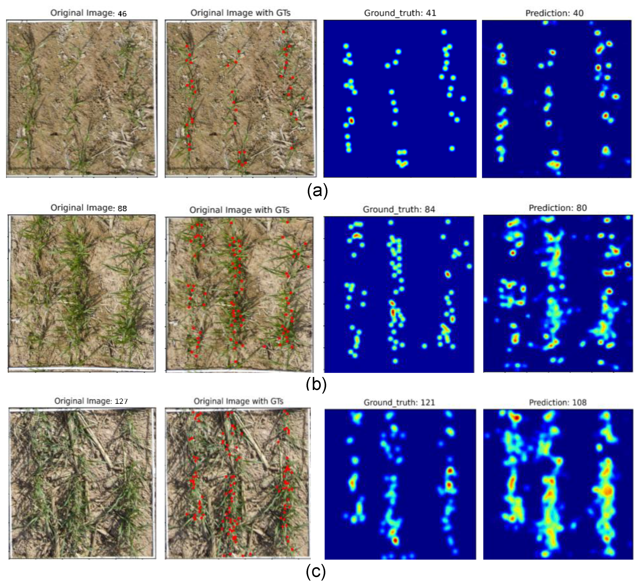
The model results showed that plant density level was critical to the model performance (Table 5). Specifically, the model degraded from the low- to high-density levels for both the sampled and annotated ground-truths. It is worth noting that the model presented a better performance on annotated ground-truth than sampled ground-truth at moderate or high plant density levels. This phenomenon could be mainly explained by the fact that plant densities were mostly underestimated on images with high plant density in the annotation (Section 3.2.1). The predicted heatmaps of different density levels also presented remarkable discrepancies (Figure 9). With higher plant density, the heatmaps would tend to include more noise in the background area. Therefore, an increase in plant density would degrade the model’s performance.

3.2.3. Impacts of Zenith Angle on Model Performance

With the low altitude of the UAV flight, the pixels on the UAV images had various zenith angles. For each quadrat, the UAV image was repeated nine times at nine specific locations to analyze the effect of the zenith angle (Section 2.1.3). According to the zenith angles, the image patches in the test dataset were divided into four parts with quadrat locations at Z1, Z2, Z3, and Z4 (with zenith angles Z1 > Z2 > Z3 > Z4).
The model results with various zenith angles presented significant differences (Table 6). Specifically, the model performance remarkably degraded with the zenith angle decrease for both the sampled and annotated ground-truths. The model reached a solid performance (MAE = 6.63, RMSE = 8.61, and R2 = 0.91) when the quadrat was located at the image center (location Z1) for the sampled ground-truth. However, the model performance was also remarkably degraded (MAE = 19.13, RMSE = 22.39, and R2 = 0.74) when the quadrat was located at the image corner (location Z4) for sampled ground-truth. The above results suggested that the zenith angle could significantly affect the model performance, and the large zenith angle boosted the model’s accuracy.

4. Discussion

4.1. Research Contributions

This study presented a deep learning model for wheat plant density estimation. Unlike traditional research that estimated wheat plant density before tillering [1,13], this study challenged the wheat density after tillering when wheat plants were highly clustered. Specifically, this study’s main research contributions are as follows. First, the results showed that the proposed DeNet was robust with the global-scale attention, outperforming the typical SegNet and U-Net network architectures. Second, this study adopted a key-point-based algorithm on plant density estimations with distinct advantages. Compared to the commonly used object detection algorithm that draws bounding-boxes around targeted plants, the key-point-based algorithm can reduce labor-cost in image annotation. Moreover, the key-point-based algorithm has the superiority in tracking dense plants in density estimation, unlike object detection algorithms mainly applied to individually presented plants on the image. Third, this study analyzed the impact of different sigma values, heatmap-assembling techniques, density levels, and zenith angles on wheat plant density estimation, providing valuable insights to future research in this domain. Fourth, the plant density estimated in this study has potential in two practical implications. Plant density after the tillering stage is a better proxy than that before the tillering stage for yield estimation, since tillers are also crucial to yield [34]. Moreover, the spatial distribution of plant density can provide guidance to precise fertilization with explicit intraspecific competition [33,50].

4.2. Potential Future Works

Although this study presented the robustness of the DeNet for wheat plant density estimation after tillering, four aspects still need further exploration for the model’s application in extensive scenarios. First, the model inheritance to a descendant or other varieties of wheat plants is still unclear since this study was limited to datasets from one year and one cultivar of wheat plants. We will collect more datasets on different cultivars in the next step to verify the model inheritance. Second, the model performance on wheat plants before tillering was not explored. It would be valuable work to comprehensively estimate wheat plant density before and after tillering, bringing more insights into the tillering mechanism [51]. Third, the plant row is meant to be extracted from the wheat heatmaps. Plant row is a significant variable in precise agricultural management [15,52]. The model-predicted heatmaps already presented an excellent distribution of plant row and are promising to be extracted in future works. Fourth, the model is essential to be applied to the field scale, as implemented in [13]. With a predefined flight path, UAVs can obtain orthomosaic images [53]. Based on the orthomosaic image, our model can potentially be applied to wheat plant density estimation on the field scale.

5. Conclusions

Unlike previous studies that generally estimated wheat plant density before tillering, this study developed a DeNet to estimate plant density after tillering. To validate the model robustness of the DeNet, the SegNet and U-Net were adopted as benchmarks to compare to the DeNet. Moreover, a sensitivity analysis was executed on the sigma value to generate ideal heatmaps. At the same time, heatmap patches were assembled based on averaging and NDIW techniques to find a better means to obtain integral heatmaps. The model evaluation on the test dataset revealed that the DeNet-estimated plant density could also well match the field-sampling-based plant density. Our test results also revealed that the plant density level and zenith angle could significantly affect the model performance. Overall, the DeNet is feasible to estimate wheat plant density after tillering on low-altitude UAV images.

Author Contributions

Conceptualization, J.P.; methodology, J.P., W.Z., E.E.R. and D.W.; resources, H.L. and B.Y.; writing—original draft preparation, J.P.; writing—review and editing, W.Z., E.E.R., D.W., H.L., B.Y. and Z.S.; supervision, Z.S.; funding acquisition, Z.S. All authors have read and agreed to the published version of the manuscript.

Funding

This work was funded by the Strategic Priority Research Program of the Chinese Academy of Sciences (XDA23050102), the National Key Research and Development Program of China (2021YFD1900902), the National Natural Science Foundation of China (31870421, 42101376), and the Program of Yellow River Delta Scholars (2020–2024).

Institutional Review Board Statement

Not applicable.

Informed Consent Statement

Not applicable.

Data Availability Statement

The data presented in this study are available on request from the corresponding author. The data are not publicly available due to Intellectual Property Regulations.

Acknowledgments

Many thanks to Da Qian, Youxiao Wang, and Peng Wang for their help in field sampling.

Conflicts of Interest

The authors declare no conflict of interest.

References

  1. Liu, S.; Baret, F.; Andrieu, B.; Burger, P.; Hemmerlé, M. Estimation of wheat plant density at early stages using high resolution imagery. Front. Plant Sci. 2017, 8, 739. [Google Scholar] [CrossRef] [Green Version]
  2. Liu, S.; Baret, F.; Allard, D.; Jin, X.; Andrieu, B.; Burger, P.; Hemmerlé, M.; Comar, A. A method to estimate plant density and plant spacing heterogeneity: Application to wheat crops. Plant Methods 2017, 13, 1–11. [Google Scholar] [CrossRef] [Green Version]
  3. Finch-Savage, W.E.; Bassel, G.W. Seed vigour and crop establishment: Extending performance beyond adaptation. J. Exp. Bot. 2016, 67, 567–591. [Google Scholar] [CrossRef] [Green Version]
  4. Karayel, D. Performance of a modified precision vacuum seeder for no-till sowing of maize and soybean. Soil Tillage Res. 2009, 104, 121–125. [Google Scholar] [CrossRef]
  5. Cowley, R.B.; Luckett, D.J.; Moroni, J.S.; Diffey, S. Use of remote sensing to determine the relationship of early vigour to grain yield in canola (Brassica napus L.) germplasm. Crop Pasture Sci. 2014, 65, 1288. [Google Scholar] [CrossRef]
  6. Zhang, D.; Luo, Z.; Liu, S.; Li, W.; Wei, T.; Dong, H. Effects of deficit irrigation and plant density on the growth, yield and fiber quality of irrigated cotton. F. Crop. Res. 2016, 197, 200–231. [Google Scholar] [CrossRef]
  7. Ren, T.; Liu, B.; Lu, J.; Deng, Z.; Li, X.; Cong, R. Optimal plant density and N fertilization to achieve higher seed yield and lower N surplus for winter oilseed rape (Brassica napus L.). F. Crop. Res. 2017, 204, 199–207. [Google Scholar] [CrossRef]
  8. Bai, Y.; Nie, C.; Wang, H.; Cheng, M.; Liu, S.; Yu, X.; Shao, M.; Wang, Z.; Wang, S.; Tuohuti, N.; et al. A fast and robust method for plant count in sunflower and maize at different seedling stages using high-resolution UAV RGB imagery. Precis. Agric. 2022, 23, 1720–1742. [Google Scholar] [CrossRef]
  9. Jin, X.; Zarco-Tejada, P.J.; Schmidhalter, U.; Reynolds, M.P.; Hawkesford, M.J.; Varshney, R.K.; Yang, T.; Nie, C.; Li, Z.; Ming, B.; et al. High-Throughput Estimation of Crop Traits: A Review of Ground and Aerial Phenotyping Platforms. IEEE Geosci. Remote Sens. Mag. 2021, 9, 200–231. [Google Scholar] [CrossRef]
  10. Mhango, J.K.; Harris, W.E.; Monaghan, J.M. Relationships between the spatio-temporal variation in reflectance data from the sentinel-2 satellite and potato (Solanum tuberosum l.) yield and stem density. Remote Sens. 2021, 13, 4371. [Google Scholar] [CrossRef]
  11. Jiang, Y.; Li, C.; Paterson, A.H.; Robertson, J.S. DeepSeedling: Deep convolutional network and Kalman filter for plant seedling detection and counting in the field. Plant Methods 2019, 15, 141. [Google Scholar] [CrossRef] [Green Version]
  12. Lu, H.; Liu, L.; Li, Y.N.; Zhao, X.M.; Wang, X.Q.; Cao, Z.G. TasselNetV3: Explainable Plant Counting with Guided Upsampling and Background Suppression. IEEE Trans. Geosci. Remote Sens. 2022, 60, 4700515. [Google Scholar] [CrossRef]
  13. Jin, X.; Liu, S.; Baret, F.; Hemerlé, M.; Comar, A. Estimates of plant density of wheat crops at emergence from very low altitude UAV imagery. Remote Sens. Environ. 2017, 198, 105–114. [Google Scholar] [CrossRef] [Green Version]
  14. Oh, S.; Chang, A.; Ashapure, A.; Jung, J.; Dube, N.; Maeda, M.; Gonzalez, D.; Landivar, J. Plant counting of cotton from UAS imagery using deep learning-based object detection framework. Remote Sens. 2020, 12, 2981. [Google Scholar] [CrossRef]
  15. Osco, L.P.; dos Santos de Arruda, M.; Gonçalves, D.N.; Dias, A.; Batistoti, J.; de Souza, M.; Gomes, F.D.G.; Ramos, A.P.M.; de Castro Jorge, L.A.; Liesenberg, V.; et al. A CNN approach to simultaneously count plants and detect plantation-rows from UAV imagery. ISPRS J. Photogramm. Remote Sens. 2021, 174, 1–17. [Google Scholar] [CrossRef]
  16. Mhango, J.K.; Harris, E.W.; Green, R.; Monaghan, J.M. Mapping potato plant density variation using aerial imagery and deep learning techniques for precision agriculture. Remote Sens. 2021, 13, 2705. [Google Scholar] [CrossRef]
  17. Valente, J.; Sari, B.; Kooistra, L.; Kramer, H.; Mücher, S. Automated crop plant counting from very high-resolution aerial imagery. Precis. Agric. 2020, 21, 1366–1384. [Google Scholar] [CrossRef]
  18. Shrestha, D.S.; Steward, B.L. Automatic corn plant population measurement using machine vision. Trans. Am. Soc. Agric. Eng. 2003, 46, 559–565. [Google Scholar] [CrossRef] [Green Version]
  19. Liu, T.; Wu, W.; Chen, W.; Sun, C.; Zhu, X.; Guo, W. Automated image-processing for counting seedlings in a wheat field. Precis. Agric. 2016, 17, 392–406. [Google Scholar] [CrossRef]
  20. Zhao, B.; Zhang, J.; Yang, C.; Zhou, G.; Ding, Y.; Shi, Y.; Zhang, D.; Xie, J.; Liao, Q. Rapeseed seedling stand counting and seeding performance evaluation at two early growth stages based on unmanned aerial vehicle imagery. Front. Plant Sci. 2018, 9, 1362. [Google Scholar] [CrossRef]
  21. Wu, F.; Wang, J.; Zhou, Y.; Song, X.; Ju, C.; Sun, C.; Liu, T. Estimation of Winter Wheat Tiller Number Based on Optimization of Gradient Vegetation Characteristics. Remote Sens. 2022, 14, 1338. [Google Scholar] [CrossRef]
  22. Zhang, J.; Yang, C.; Song, H.; Hoffmann, W.C.; Zhang, D.; Zhang, G. Evaluation of an airborne remote sensing platform consisting of two consumer-grade cameras for crop identification. Remote Sens. 2016, 8, 257. [Google Scholar] [CrossRef] [Green Version]
  23. Banerjee, B.P.; Sharma, V.; Spangenberg, G.; Kant, S. Machine learning regression analysis for estimation of crop emergence using multispectral uav imagery. Remote Sens. 2021, 13, 2918. [Google Scholar] [CrossRef]
  24. LeCun, Y.; Bengio, Y.; Hinton, G. Deep learning. Nature 2015, 521, 436–444. [Google Scholar] [CrossRef]
  25. Zhang, L.; Zhang, L.; Du, B. Deep learning for remote sensing data: A technical tutorial on the state of the art. IEEE Geosci. Remote Sens. Mag. 2016, 4, 22–40. [Google Scholar] [CrossRef]
  26. Kitano, B.T.; Mendes, C.C.T.; Geus, A.R.; Oliveira, H.C.; Souza, J.R. Corn Plant Counting Using Deep Learning and UAV Images. IEEE Geosci. Remote Sens. Lett. 2019, 16, 1–5. [Google Scholar] [CrossRef]
  27. Redmon, J.; Farhadi, A. YOLOv3: An Incremental Improvement. arXiv 2018, arXiv:1804.02767. [Google Scholar]
  28. Machefer, M.; Lemarchand, F.; Bonnefond, V.; Hitchins, A.; Sidiropoulos, P. Mask R-CNN refitting strategy for plant counting and sizing in uav imagery. Remote Sens. 2020, 12, 3015. [Google Scholar] [CrossRef]
  29. He, K.; Gkioxari, G.; Dollar, P.; Girshick, R. Mask R-CNN. In Proceedings of the 2017 IEEE International Conference on Computer Vision (ICCV), Venice, Italy, 22–29 October 2017; pp. 2961–2969. [Google Scholar] [CrossRef]
  30. Longnecker, N.; Kirby, E.J.M.; Robson, A. Leaf Emergence, Tiller Growth, and Apical Development of Nitrogen-Dificient Spring Wheat. Crop Sci. 1993, 33, 154–160. [Google Scholar] [CrossRef]
  31. Maas, E.V.; Lesch, S.M.; Francois, L.E.; Grieve, C.M. Tiller development in salt-stressed wheat. Crop Sci. 1994, 34, 1594–1603. [Google Scholar] [CrossRef]
  32. Rodríguez, D.; Andrade, F.H.; Goudriaan, J. Effects of phosphorus nutrition on tiller emergence in wheat. Plant Soil 1999, 209, 283–295. [Google Scholar] [CrossRef]
  33. Ding, Y.; Zhang, X.; Ma, Q.; Li, F.; Tao, R.; Zhu, M.; Li, C.; Zhu, X.; Guo, W.; Ding, J. Tiller fertility is critical for improving grain yield, photosynthesis and nitrogen efficiency in wheat. J. Integr. Agric. 2022, 21. [Google Scholar] [CrossRef]
  34. Bastos, L.M.; Carciochi, W.; Lollato, R.P.; Jaenisch, B.R.; Rezende, C.R.; Schwalbert, R.; Vara Prasad, P.V.; Zhang, G.; Fritz, A.K.; Foster, C.; et al. Winter Wheat Yield Response to Plant Density as a Function of Yield Environment and Tillering Potential: A Review and Field Studies. Front. Plant Sci. 2020, 11, 54. [Google Scholar] [CrossRef] [PubMed] [Green Version]
  35. Badrinarayanan, V.; Kendall, A.; Cipolla, R. SegNet: A Deep Convolutional Encoder-Decoder Architecture for Image Segmentation. IEEE Trans. Pattern Anal. Mach. Intell. 2017, 39, 2481–2495. [Google Scholar] [CrossRef] [PubMed]
  36. Ronneberger, O.; Fischer, P.; Brox, T. U-Net: Convolutional Networks for Biomedical Image Segmentation. In Lecture Notes in Computer Science (Including Subseries Lecture Notes in Artificial Intelligence and Lecture Notes in Bioinformatics); Navab, N., Hornegger, J., Wells, W.M., Frangi, A.F., Eds.; Lecture Notes in Computer Science; Springer International Publishing: Cham, Switzerland, 2015; Volume 9351, pp. 234–241. ISBN 978-3-319-24573-7. [Google Scholar]
  37. Peterson, C.M.; Klepper, B.; Rickman, R.W. Tiller Development at the Coleoptilar Node in Winter Wheat 1. Agron. J. 1982, 74, 781–784. [Google Scholar] [CrossRef]
  38. NVIDIA Developer CUDA. Available online: https://developer.nvidia.com/cuda-toolkit (accessed on 5 September 2022).
  39. Peng, J.; Wang, D.; Liao, X.; Shao, Q.; Sun, Z.; Yue, H.; Ye, H. Wild animal survey using UAS imagery and deep learning: Modified Faster R-CNN for kiang detection in Tibetan Plateau. ISPRS J. Photogramm. Remote Sens. 2020, 169, 364–376. [Google Scholar] [CrossRef]
  40. Russell, B.C.; Torralba, A.; Murphy, K.P.; Freeman, W.T. LabelMe: A Database and Web-Based Tool for Image Annotation. Int. J. Comput. Vis. 2008, 77, 157–173. [Google Scholar] [CrossRef]
  41. Karen, S.; Andrew, Z. Very deep convolutional networks for large-scale image recognition. arXiv 2015, arXiv:1409.1556. [Google Scholar]
  42. Hossain, M.A.; Hosseinzadeh, M.; Chanda, O.; Wang, Y. Crowd counting using scale-aware attention networks. In Proceedings of the 2019 IEEE winter conference on applications of computer vision (WACV), Waikoloa Village, HI, USA, 7–11 January 2019; pp. 1280–1288. [Google Scholar] [CrossRef] [Green Version]
  43. Sam, D.B.; Surya, S.; Babu, R.V. Switching convolutional neural network for crowd counting. In Proceedings of the 2017 IEEE Conference on Computer Vision and Pattern Recognition (CVPR), Honolulu, HI, USA, 21–26 July 2017; pp. 4031–4039. [Google Scholar] [CrossRef] [Green Version]
  44. Sindagi, V.A.; Patel, V.M. Generating High-Quality Crowd Density Maps Using Contextual Pyramid CNNs. In Proceedings of the 2017 IEEE International Conference on Computer Vision (ICCV), Venice, Italy, 22–29 October 2017; pp. 1879–1888. [Google Scholar] [CrossRef]
  45. Bendali-Braham, M.; Weber, J.; Forestier, G.; Idoumghar, L.; Muller, P.-A. Recent trends in crowd analysis: A review. Mach. Learn. Appl. 2021, 4, 100023. [Google Scholar] [CrossRef]
  46. Munea, T.L.; Jembre, Y.Z.; Weldegebriel, H.T.; Chen, L.; Huang, C.; Yang, C. The Progress of Human Pose Estimation: A Survey and Taxonomy of Models Applied in 2D Human Pose Estimation. IEEE Access 2020, 8, 133330–133348. [Google Scholar] [CrossRef]
  47. Duan, K.; Bai, S.; Xie, L.; Qi, H.; Huang, Q.; Tian, Q. CenterNet: Keypoint triplets for object detection. In Proceedings of the 2019 IEEE/CVF International Conference on Computer Vision (ICCV), Seoul, South Korea, 27–28 October 2019; pp. 6568–6577. [Google Scholar] [CrossRef] [Green Version]
  48. Keras Google Group. Available online: https://keras.io/ (accessed on 8 September 2022).
  49. Kingma, D.P.; Ba, J.L. Adam: A method for stochastic optimization. arXiv 2015, arXiv:1412.6980. [Google Scholar]
  50. Fischer, R.A.; Moreno Ramos, O.H.; Ortiz Monasterio, I.; Sayre, K.D. Yield response to plant density, row spacing and raised beds in low latitude spring wheat with ample soil resources: An update. F. Crop. Res. 2019, 232, 95–105. [Google Scholar] [CrossRef]
  51. Liu, T.; Zhao, Y.; Wu, F.; Wang, J.; Chen, C.; Zhou, Y.; Ju, C.; Huo, Z.; Zhong, X.; Liu, S.; et al. The estimation of wheat tiller number based on UAV images and gradual change features (GCFs). Precis. Agric. 2022, 23, 1–22. [Google Scholar] [CrossRef]
  52. Che, Y.; Wang, Q.; Zhou, L.; Wang, X.; Li, B.; Ma, Y. The effect of growth stage and plant counting accuracy of maize inbred lines on LAI and biomass prediction. Precis. Agric. 2022, 23, 1–27. [Google Scholar] [CrossRef]
  53. Mills, S.; McLeod, P. Global seamline networks for orthomosaic generation via local search. ISPRS J. Photogramm. Remote Sens. 2013, 75, 101–111. [Google Scholar] [CrossRef]
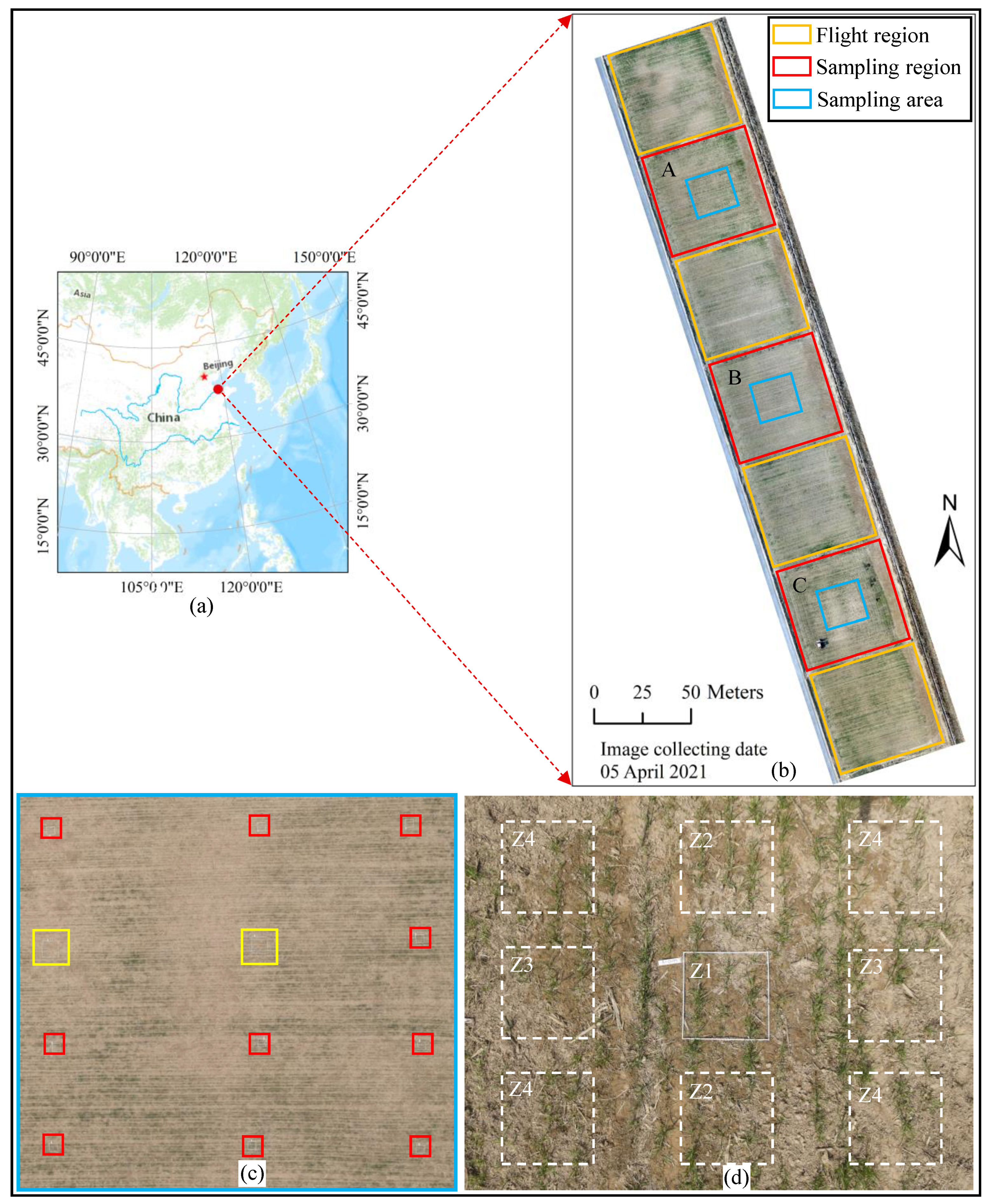
Figure 1. (a) Overview of study area location in China. (b) Seven patches of wheat farming fields with orange boxes and red boxes represent flight and sampling regions, respectively. The blue box indicates the area containing sampling quadrats with more details in (c). (c) The distribution of 12 quadrats (ten red boxes indicate ten 0.5 m × 0.5 m sampling quadrats adopted, and two yellow boxes indicate two 1 m × 1 m sampling quadrats abandoned because of unsuitable size for deep learning models). (d) A UAV full image with a sampling quadrat located in the center (Z1) and other eight quadrat-distributing locations on corresponding images indicated by white dash boxes (Z2, Z3, and Z4).
Remotesensing 14 05923 g001
Figure 2. An overview of UAV image splitting with overlay (purple strips). The red box emphasizes an image patch with wheat plants annotated.
Remotesensing 14 05923 g002
Figure 3. (a) An overview of the workflow for plant density estimation and network architecture of three models used in this study. (b) DeNet, (c) U-Net, and (d) SegNet. The m and n in the ‘m/n’ label at the upper left of each layer represent layer channel number and down-sampling stride, respectively. GT represents ground-truth.
Remotesensing 14 05923 g003
Figure 4. The loss changes in model training of three models with the blue, purple, and black circles indicate the general locations of model convergence for SegNet, U-Net, and DeNet, respectively.
Remotesensing 14 05923 g004
Figure 5. Examples of model prediction from three models. (a) An example of an original image patch in the validation dataset. (b) Original image patch with annotations. (c) Heatmap generated from annotations. (d) Heatmap predicted by SegNet. (e) Heatmap predicted by U-Net. (f) Heatmap predicted by DeNet. The number in the upper image indicates plant density in the image patch (ground-truth or prediction).
Remotesensing 14 05923 g005
Figure 6. Examples of DeNet predictions with different sigma values in sensitivity analysis (4, 8, 12, 14, 15, 16, 17, 18, 20, and 24). (a) An example of an original image patch in the validation dataset. (b) The image patches with annotations. (c,e,g,i,k,m,o,q,s,u): heatmap generated from ground-truth with different sigma values. (d,f,h,j,l,n,p,r,t,v): heatmap predicted from the plant density model with different sigma values. GT: ground-truth; pre: predicted plant density.
Remotesensing 14 05923 g006
Figure 7. Heatmap assembling results in different assembling techniques. (a) A full image in the validation dataset. (b) The heatmap from annotated points. (c) The assembled heatmap using the averaging technique with the predicted heatmap. (d) The assembled heatmap using the NIDW technique with the predicted heatmap.
Remotesensing 14 05923 g007
Figure 8. The plant density comparison between (a) sampled GT and annotated GT, (b) annotated GT and prediction, and (c) sampled GT and prediction on the test dataset. GT represents ground-truth.
Remotesensing 14 05923 g008
Figure 9. Examples of wheat plant density estimation on the test dataset with different density levels: (a) low, (b) moderate, and (c) high plant density levels.
Remotesensing 14 05923 g009
Table 1. A brief introduction of UAV datasets used in this study.
DatasetQuadratFull ImagePatchPatch SizeUsage
TrainingNo8525501200 × 1200Model training
ValidationNo15945~1200 × 1200Model validation
TestYes270270~1200 to 1300 Model test
Quadrat: containing a sampling quadrat or not in the image; full image: total number counting of the used full UAV images; Patch: total number counting of the used image patches; Patch size: image patch resolution or height (or width) with the unit of ‘pixel’. The symbol ‘~’ indicates an approximate value.
Table 2. The prediction results of three models assessed on the validation dataset.
ModelTimeGTPRMAERMSER2
SegNet8.835,43530,38618.28 21.12 0.72
U-Net9.135,43532,78914.05 20.38 0.75
DeNet9.535,43535,96112.63 17.25 0.79
Time: training time per epoch (minute), GT: total number of ground-truth, PR: total number of predictions. The unit of MAE and RMSE was ‘plants/patch’.
Table 3. The sensitivity analysis results of the sigma values evaluated using the validation dataset.
RoundSigma ValueGTPRMAERMSER2
First round435,43527,69921.94 26.88 0.73
835,43528,42920.26 25.30 0.76
1235,43533,42313.19 18.34 0.78
1635,43535,38712.11 16.21 0.82
2035,43535,53815.48 19.78 0.74
2435,43539,62117.67 22.74 0.72
Second round1435,43535,72713.04 17.24 0.73
1535,43535,96112.63 17.25 0.79
1735,43535,59212.34 16.78 0.78
1835,43536,25923.37 27.67 0.73
GT: the total number of ground-truths; PR: the total number of model predictions. The unit of MAE and RMSE was ‘plants/patch’.
Table 4. The model performance with different assembling techniques on the validation dataset.
Assembling TechniquesGTPRMAERMSER2
Averaging26,58226,51211.87 16.13 0.82
NIDW26,58226,56211.34 15.940.83
Not assembled35,43535,38712.11 16.21 0.82
NIDW: normalized inverse distance weighted.
Table 5. The model performance on different density levels.
Evaluation MatrixDensity LevelGTPRMAERMSER2
Sampled GTLow700264749.35 11.510.29
Moderate6300519012.6814.930.25
High7749708815.38 18.870.22
Annotated GTLow659064749.4011.500.33
Moderate5758519010.7612.910.30
High6788708811.8518.870.17
Table 6. The influences of zenith angle on model performance.
Evaluation MatrixQuadrat LocationGTPRMAERMSER2
Sampled GTZ1233920526.638.610.91
Z24678435612.5013.150.86
Z34678432414.8017.89 0.84
Z49356778619.13 22.390.74
Annotated GTZ1204720527.178.820.88
Z24230435610.1011.880.86
Z34327455814.1318.360.83
Z48532778618.2321.050.78
Publisher’s Note: MDPI stays neutral with regard to jurisdictional claims in published maps and institutional affiliations.