Article

Application of 3D Error Diagram in Thermal Infrared Earthquake Prediction: Qinghai–Tibet Plateau

1
School of Science, China University of Geosciences (Beijing), Beijing 100083, China
2
Aerospace Information Research Institute, Chinese Academy of Sciences, Beijing 100094, China
3
Key Laboratory of Earth Observation of Hainan Province, Hainan Aerospace Information Research Institute, Sanya 572029, China
4
Department of Geophysics, School Earth and Space Sciences, Peking University, Beijing 100089, China
5
Environment & Climate Changes Research Institute, National Water Research Center, El Qanater EI Khairiya 13621/5, Egypt
6
College of Engineering, Tibet University, Lhasa 850001, China
7
China Earthquake Networks Center, Beijing 100045, China
*
Author to whom correspondence should be addressed.
Remote Sens. 2022, 14(23), 5925; https://doi.org/10.3390/rs14235925
Submission received: 30 September 2022 / Revised: 6 November 2022 / Accepted: 9 November 2022 / Published: 23 November 2022

Abstract

:
Earthquakes are the most dangerous natural disasters, and scholars try to predict them to protect lives and property. Recently, a long-term statistical analysis based on a “heating core” filter was applied to explore thermal anomalies related to earthquakes; however, some gaps are still present. Specifically, (1) whether there are differences in thermal anomalies generated by earthquakes of different magnitudes has not yet been discussed; and (2) thermal anomalies in high-spatial-resolution data are often distributed in spots, which is not convenient for statistics of thermal anomalies. To address these issues, in this study, we applied high-spatial-resolution thermal infrared data to explore the performance of the “heating core” for earthquake prediction at different magnitudes (i.e., 3, 3.5, 4, 4.5, and 5). The specific steps were as follows: first, the resampling and moving-window methods were applied to reduce the spatial resolution of the dataset and extract the suspected thermal anomalies; second, the “heating core” filter was used to eliminate thermal noise unrelated to the seismic activity in order to identify potential thermal anomalies; third, the time–distance–magnitude (TDM) windows were used to establish the correspondence between earthquakes and thermal anomalies; finally, the new 3D error diagram (false discovery rate, false negative rate, and space–time correlation window) and the significance test method were applied to investigate the performance under each minimum magnitude with training data, and the robustness was validated using a test dataset. The results show that the following: (1) there is no obvious difference in the thermal anomalies produced by earthquakes of different magnitudes under the conditions of a “heating core”, and (2) the best model with a “heating core” can predict earthquakes effectively within 200 km and within 20 days of thermal anomalies’ appearance. The binary prediction model with a “heating core” based on thermal infrared anomalies can provide some reference for earthquake prediction.

Graphical Abstract

1. Introduction

Earthquakes, as natural disasters, are always a threat to the safety of human life and property. Confronted with the disasters brought about by earthquakes, there is an urgent need for research on earthquake precursors in order to improve the science and accuracy of earthquake prediction. With the rapid development of remote sensing, the use of TIR anomalies (TIRAs) based on remote sensing as earthquake precursors was proposed by Gorny [1] in 1988. There are some hypotheses about seismic thermal anomalies, such as the one on “P-holes” [2]. This hypothesis posits that the increase in ground stress affects the proxy bond in rocks before earthquakes, leading to the occurrence of holes due to the electron transfer in rocks and the formation of connecting circuits in the crust, thereby generating an electric current and causing thermal anomalies. Since then, multisource satellite data have been widely used to study the TIRAs of earthquakes, such as data obtained from the Moderate-Resolution Imaging Spectroradiometer (MODIS) sensors on the Terra and Aqua satellites, the Advanced Very-High-Resolution Radiometer/2/3 (AVHRR/2/3) on the NOAA satellites, the Visible and Infrared Spin Scan Radiometer (VISSR) on FY-2, and the Medium-Resolution Spectral Imager (MERSI) on FY-3.
In the past 30 years, researchers have conducted experiments to explore the relationships between earthquakes and TIRAs [3,4,5,6,7,8,9,10,11,12,13]. For example, Zhang et al. [10] used NCEP (National Centers for Environmental Prediction) temperature data to analyze the multilayer temperature changes before and after the 2014 Ludian earthquake in Yunnan, using significance tests to verify that the TIRAs before the Ludian earthquake were not accidental. Lu et al. [4] analyzed the TIRAs of 20 moderate-to-strong earthquakes in the Tibetan region from 2010 to 2015 using microwave brightness temperature (MBT) and outgoing longwave radiation (OLR), and the results showed that most of the earthquakes were preceded by TIRAs. Zhong et al. [5] simultaneously investigated the TEC and TIR during the 2017 Jiuzhaigou earthquake. The experimental results showed that a large range of TEC anomalies appeared south of the epicenter, and the intensity of the anomalies south of the Huarong Mountain rupture was the largest and overlapped with the area of the TIRAs. Using land surface temperature remote sensing data as inputs, Peleli et al. [13] applied the robust satellite technique (RST) method to detect thermal anomalies in an earthquake, and they concluded that the thermal anomalies might be connected with the gas release that takes place due to stress changes and is controlled by the existence of tectonic lines and the density of the faults.
However, most of the current research focuses only on the cases with TIRAs and ignores the earthquakes without TIRAs. Therefore, an individual earthquake case analysis cannot be used to prove the correlation between earthquakes and TIRAs. To evaluate the relationship between earthquakes and thermal anomalies more fairly, the importance of conducting long-term data analysis rather than occasional attempts must be emphasized. Some scholars [14,15,16,17,18,19,20] have studied the correlation between thermal anomalies and earthquakes in long-term statistical analyses and tried to prove the correlation between earthquakes and thermal anomalies from a statistical point of view. Among them, the Molchan diagram (MD) [21,22]—a plot of the false negative rate (FNR) vs. the fraction of time occupied by alarms, and the receiver operating characteristic (ROC) [23]—a plot of the true positive rate (TPR) vs. the false positive rate (FPR), have been adapted to prove the relationship between earthquakes and thermal anomalies. For example, Eleftheriou et al. [19] carried out a long-term time-series study of TIRAs in the Greek region between 2004 and 2013 based on the RST (robust satellite technique) algorithm, and the results of the MD showed that the correlation between earthquakes and TIRAs was not coincidental, although a large number of seismic events were underreported due to cloud cover occlusion. Fu et al. [16] used outgoing longwave radiation (OLR) data in Taiwan from 2009 to 2019 to extract thermal anomalies, where only the FNR was used for evaluating the correlation between earthquakes and thermal anomalies, and the evaluation of the false discovery rate (FDR) was ignored. The MD was used to evaluate the performance of the model based only on the FNR, ignoring the importance of the FDR. A high FDR indicates that the model is unable to filter out the seismic-related thermal anomalies from a large number of thermal anomalies. However, Zhang et al. [24] proved that the FDR and FNR are independent of one another. People will not trust alarms with a high FDR, even when the FNR of these alarms is low. In addition to the integrity of the evaluation indicators, their statistical methods are also essential. Zhang et al. [18] repeated the experiments reported in [19] and evaluated the performance of these alarms with the MD weighted by the relative intensity (RI) index, among other methods; the results of the repeated experiments indicate that these alarms perform no better than a random guess. Unlike the original MD, the RI-weighted MD [25] accounts for the prior spatial distribution of earthquakes, where the RI quantifies the historical seismicity rates [26]. The original MD may offer inaccurate results for inhomogeneous spatial systems, while this RI-weighted MD has also been found to be effective for statistical analysis [18].
In addition, with the development of artificial intelligence, machine learning and deep learning methods are increasingly being applied to earthquake prediction research [27,28,29,30,31,32,33,34]. For example, DeVries et al. [27] and Mignan et al. [28] constructed deep learning models to predict the spatial distribution of aftershocks and evaluated the performance of their models using the ROC. However, Parsons [35] indicated that the ROC test was ineffective for evaluating the alarms when the earthquake distribution was spatially imbalanced. Shodiq et al. [33] proposed an adaptive neuro-fuzzy inference system (ANFIS) based on automatic clustering for earthquake prediction in Indonesia, and its accuracy was 70%. Jiang et al. [34] constructed a support vector machine (SVM) to predict earthquakes in southern China; a total of 39 earthquake cases were used, and the tests showed that the model had a recall of 50%; however, the spatial distribution of the reference models for these metrics was homogeneous.
To address the shortcomings of the above metrics for earthquake prediction, Zhang et al. [24] proposed a 3D error diagram and a method for testing the significance of inhomogeneous Poisson distribution to evaluate the performance of the earthquake prediction. Among them, the FNR significance test was proposed by Zechar and Jordan [25].
In the extraction of the TIRAs, not all thermal anomalies are associated with seismic activity due to human activities and weather effects. For example, lateral movements of hot air masses and other meteorological warming processes can also produce TIRAs [36,37,38]. Therefore, thermal anomalies include both seismic-related thermal anomalies—which are often referred to as “signals”—and non-seismic-related thermal anomalies, which are referred to as “noise”. To improve the signal/noise (S/N) ratio of TIRAs and obtain reliable alarms, some scholars have eliminated irrelevant thermal anomalies by setting a series of conditions, such as intensity and time continuity [15,17,19,39,40].
A large number of studies have focused on the correlation between thermal anomalies and earthquakes, while less discussion has been devoted to the thermal anomalies generated by earthquakes of different magnitudes. In addition, medium- and low-resolution data, such as OLR, have often been used for long-term statistical analysis [15,16]. For high-spatial-resolution TIR data, thermal anomalies are difficult to number and statistically analyze.
In this study, first, thermal infrared data from historical periods were used to construct a background field to extract suspected thermal infrared anomalies (STIRAs). Secondly, two downscaling methods—resampling and moving windows—were used to reduce the spatial resolution of the data, each with two scales of 50 km and 100 km, so as to facilitate the integration of discrete thermal anomalies. Then, the thermal noise in the TIRAs was removed using a “heated core” filter [15], and the screened TIRAs were called potential TIRAs (PTIRAs). In addition, the time–distance–magnitude (TDM) windows were used to judge whether the earthquake was related to STIRAs or PTIRAs. Finally, to obtain the optimal parameters, a training–test method was used to divide the data into a training dataset and a testing dataset. At the same time, the 3D error diagram was used to select the optimal parameters in the training dataset to form the optimal binary earthquake prediction model, and the testing dataset was used to verify whether the optimal model could achieve effective predictions. The data from January 2014 to December 2016 were used as the training dataset, while the data from January 2017 to December 2019 were used as the testing dataset.
In this paper, we first introduce the TIR dataset used to extract thermal anomalies and the geological background of the Qinghai–Tibet Plateau in Section 2. Then, in Section 3, we introduce the rule of “heating core” under two downscaling conditions—resampling and moving windows—as well as the evaluation method for the models. To explore the performance of the “heating core” under different magnitudes, the results of four sets of comparative experiments with and without the “heating core” are shown in Section 4. Finally, the discussion and conclusions of this study are detailed in Section 5 and Section 6, respectively.

2. Dataset and Study Area

Many studies have shown the influence of clouds on thermal infrared data [36,41,42] and found that the presence of TIRAs is influenced by cloud cover. As reported, the percentage of cloud coverage over the Qinghai–Tibet Plateau exceeds 50%, which is above the global average [43]. The amount of seismic thermal anomaly information cannot be effectively observed, as shown in Figure 1. To monitor the temporal and spatial changes in thermal anomalies caused by earthquakes more comprehensively and continuously, we used TRIMS LST (Thermal and Reanalysis Integrating Moderate-resolution Spatial-seamless LST), which was introduced by Zhang et al. [44,45,46]. The dataset was applied to merge aqua/terra Moderate-Resolution Imaging Spectroradiometer (MODIS) and Global/China Land Data Assimilation System (GLDAS/CLDAS) data over the Tibetan Plateau and the surrounding area. Then, the high- and low-frequency components of the surface temperature, along with the spatial correlation of the surface temperature provided by satellite thermal infrared remote sensing and reanalysis data, were used to develop a higher-quality all-weather surface temperature dataset. The RMSE (root-mean-square error) of the measured data from the ground station was 1.52–3.71 K, which satisfies the accuracy requirements of this study. The spatial resolution of the data was 1 km × 1 km, with approximate observation times at 10:30 a.m./1:30 p.m. (local solar time) in ascending orbit and 10:30 p.m./1:30 a.m. in descending orbit. The data were downloaded from the “National Qinghai–Tibet Plateau Science Data Center”, accessed on 20 August 2021 (http://data.tpdc.ac.cn, accessed on 25 June 2022) [47]. As the daytime data are badly affected by the Sun, we chose the daily nighttime TRIMS LST data to extract the TIRAs before earthquakes.
The Qinghai–Tibet Plateau (26°N–40°N, 73°E–105°E) is one of the four main geographic regions in China. It is located to the west of the Hengduan Mountains, north of the Himalayas, and south of the Kunlun Mountains, Altun Mountains, and Qilian Mountains. The Qinghai–Tibet Plateau is characterized by seismic activities with high magnitude and a high frequency of earthquakes. Between 2000 and 2019, there were 200 earthquakes of magnitude 5; the highest earthquake magnitude was 8.1, causing great loss of life and economic damage. The earthquake catalog of the Qinghai–Tibet Plateau was provided by the China Earthquake Data Center (http://data.earthquake.cn, accessed on 22 June 2022). This study focused on the seismic data of the Tibetan Plateau with a magnitude 3 and a depth > 0, during the period from 2014 to 2019. The total number of earthquakes that met the selected criteria was 1377.
The completeness of the seismic catalog is crucial. To assess the spatial and temporal relationships between earthquakes and thermal anomalies accurately, and to reduce the occurrence of “false alarms” due to incomplete earthquake catalogs, the Gutenberg–Richter law [48]—which describes the magnitude of an earthquake as an exponential distribution, l o g N = a b M (where N is the total number of earthquakes with magnitude ≥ M)—was used to assess the completeness of the catalog. As shown in Figure 2b, this study analyzed the completeness of earthquakes of magnitude 3 and above from 2000 to 2019, and the results showed that there was a significant exponential relationship between the number of earthquakes and their magnitude and that the catalog was complete when the earthquakes were of magnitude 3 and above.
The physical mechanisms of all earthquakes—including foreshocks, mainshocks, and aftershocks—should be the same [49,50], although some studies do not fully agree with this assessment [51,52,53]. The seismic thermal anomaly precursors should be related to the accumulation and release of seismic energy, i.e., the precursors should be related to the magnitude of the earthquake and not to its mainshock or aftershock. The de-clustering approach would hide the potential relationships between some TIRAs and the “removed earthquakes”. To investigate the effects of seismic catalog de-clustering on the performance analysis of seismic thermal anomalies, Zhang [54] used four different de-clustering methods (window methods [55,56,57], Reasenberg’s methods [58], single-link cluster analysis [59], and Zaliapin’s method [60,61]) to process the seismic catalogs. It was found that there were significant differences between the obtained catalogs and that the seismic catalog de-clustering methods can bring instability to the evaluation of seismic thermal anomalies. Therefore, Zhang [54] recommends not preprocessing the seismic catalogs with de-clustering when evaluating alert performance. For a more complete assessment of the correlation between seismic thermal anomalies and earthquakes, the seismic catalogs in this experiment were not de-clustering.

3. Methodology

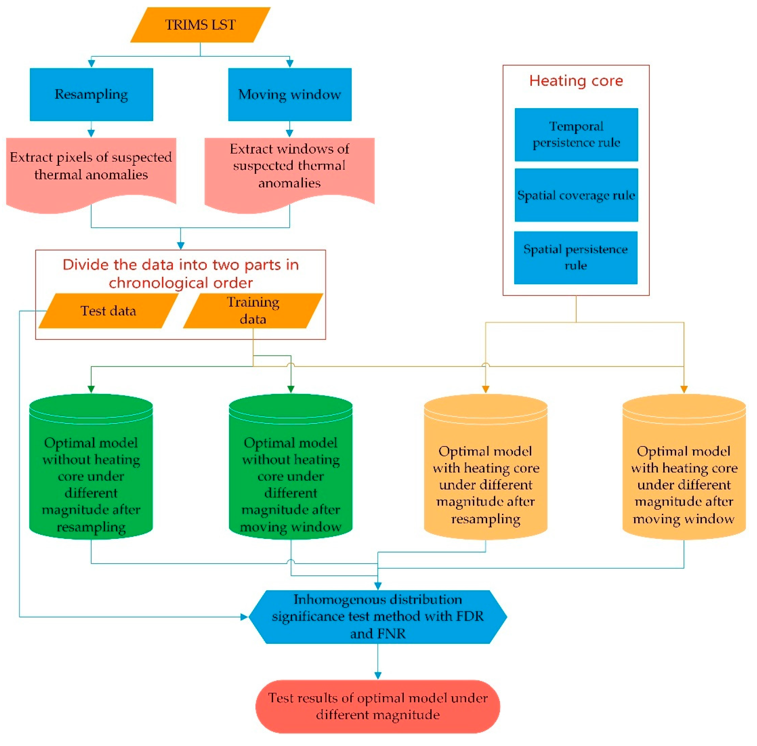
Due to the high spatial resolution of TRIMS LST, firstly, resampling and moving windows were applied to reduce the spatial resolution of the dataset and extract the thermal anomalies to obtain STIRAPs (suspected thermal infrared anomaly patches). Secondly, the “heating core” filter—including the temporal persistence rule, spatial coverage rule, and spatial persistence rule—was used to eliminate thermal noise unrelated to the seismic activity in order to obtain PTIRAPs (potential thermal infrared anomaly patches). Then, we established correspondence between STIRAPs or PTIRAPs and earthquakes, including the predicted spatiotemporal window TD and the magnitude M. Finally, a 3D error diagram (e.g., FDR, FNR, STCW) and significance tests for FDR/FNR were used to evaluate the performance of earthquake prediction. In addition, based on the training dataset, the optimal models with and without a “heating core” were selected under different minimum magnitudes, and the testing dataset was used to validate the models. The flowchart is shown in Figure 3.

3.1. Thermal Anomaly Extraction Based on Resampling and Moving Windows

TIRAs are supposed to be caused by the direct or indirect influence of increasing crustal stress [18]. Therefore, the mean daily data for years with fewer earthquakes were used to calculate the TIR background field. Based on the statistics of the earthquake catalog from 2000 to 2019, as shown in Figure 2, the number of earthquakes between 2000 and 2005 was relatively small, so the data from this period were selected. T I R r e f ( x , y , t ) represents the temperature of the TIR background field at (x, y) on day t; T I R ( x , y , t , i ) represents the surface temperature at (x, y) in the year i on day t; and a and b represent the start and end years of the data used to calculate the TIR background field, respectively.
T I R r e f ( x , y , t ) = 1 b a + 1 i = a b T I R ( x , y , t , i )
where θ is the threshold value of the exception; if the T I R ( x , y , t , j ) > T I R r e f ( x , y , t ) + θ , j { 2014 ,   2015 ,   2016 ,   2017 ,   2018 ,   2019 } , then T I R ( x , y , t , j ) will be regarded as a STIRA at location ( x , y ) on day i , and it is possibly related to the earthquake.
For the resampling method, γ is the resampling parameter; that is, the spatial resolution of the original data is reduced by a factor of γ. The resampled data are used to calculate the TIR background field to extract the STIRA. Under this method, ( x , y ) in Formula (1) represents the coordinate value after resampling, and the extraction of the STIRA depends on the parameters ( γ , θ ) .
For the moving window, ( x , y ) in Formula (1) is the original coordinate value; that is, the original high-spatial-resolution TIR data are used to calculate the TIR background field and the anomaly pixels. The pixels are marked as 1 if T I R ( x , y , t , j ) > T I R r e f ( x , y , t ) + θ , and 0 otherwise. Then, a moving window whose width and step length are both s is used to calculate the ratio r of the anomaly pixels to all valid pixels in each window, where f l a g ( x , y , t , j ) represents the mark of the anomaly pixel at (x, y) in the year j and on day t, while n u m b e r ( T I R ( m , n , t , j ) ) represents the number of valid pixels; (m, n) represents the row and column numbers where the moving window is located, and its value range is shown in Formula (3), where N represents a set of natural numbers. μ is the thermal anomaly ratio threshold; the moving window is considered to be the STIRA if the ratio r is greater than μ , and the extraction of the STIRA depends on the parameters ( s , θ , μ ) .
r = x = m × s ( m + 1 ) × s y = n × s ( n + 1 ) × s f l a g ( x , y , t , j ) n u m b e r ( T I R ( m , n , t , j ) )
{ m [ 1 , i n t ( max ( x ) s 1 ) ] N n [ 1 , i n t ( max ( y ) s 1 ) ] N
For each day, these spatial adjacent TIRAs form many patches, which are regarded as “suspected TIRA patches” (STIRAPs). Then, we assign a different number for each spatially separate STIRAP on each day. For example, STIRAP i , α indicates that the number of STIRAPs this patch is α on day i .

3.2. Thermal Anomaly Filtering

The concept of “heating core”, as described by Zhang et al. [15], is used as a reference in this paper. It assumes that the TIRAPs caused by earthquakes should be persistent in time and space. To extract the TIRAPs that may be related to earthquakes and to remove thermal noise that may not be related to earthquakes, a series of spatiotemporal rules—including temporal persistence, spatial coverage, and spatial persistence—are set. Only if the STIRAPs satisfy the following rules are they regarded as the PTIRAPs that may be related to earthquakes:
Temporal persistence rule: PTIRAPs should last for at least two days in the same area.
β R , STIRAP i , α STIRAP i + 1 , α
Spatial coverage rule: The influence range of an earthquake is limited due to the earthquake being a local geological movement; therefore, the area of each PTIRAP should be larger than a r e a m i n and smaller than a r e a m a x .
a r e a m i n A R E A ( STIRAP i , α ) a r e a m a x
Spatial persistence rule: The PTIRAPs should be persistent in space; that is, the overlapped area of PTIRAPs in two consecutive days should be greater than a threshold. Unlike the conditions of the original rule, we introduce a stricter factor i o u (intersection over union) (0 ≤ i o u ≤ 1) to help us determine the threshold.
A R E A ( STIRAP i , α STIRAP i + 1 , β ) A R E A ( STIRAP i , α STIRAP i + 1 , β ) > i o u
All of the STIRAPs are filtered by the above three conditions, and the STIRAP that passes the filtering is called a PTIRAP; in other words, PIRAPs are the result of STIRAP refinement. Each STIRAP or PTRIAP serves as an alarm for the model without a “heating core” and the model with a “heating core”, respectively.

3.3. Correspondence between Earthquakes and Thermal Anomalies

The time–distance–magnitude (TDM) windows judge whether the alarm is related to the earthquake. T and D represent the time and distance ranges for warning after the alarm occurs, respectively, while M represents the minimum magnitude for participating in training and testing. If an earthquake of magnitude M or above occurs within the spatiotemporal range after an alarm appears, the alarm is considered to correspond to the earthquake; in this case, the alarm is called a successful alarm, and the earthquake is called a successfully predicted event. Otherwise, the alarm is called a false alarm. In addition, if the earthquake is not alerted by the spatial and temporal range of any alarm, then the earthquake is called a missing event. The specific forms of the three rules are as follows:
Temporal rule: T f i r s t < t e T l a s t + T , where T f i r s t and T l a s t represent the first and last days of the alarm, respectively, while t e denotes the time of the earthquake.
Distance rule: The Euclidean distance between the epicenter of E Q ( x , y , t , m ) and any pixel of the alarm is less than or equal to D. E Q ( x , y , t , m ) means that an earthquake with an epicenter of ( x , y ) and magnitude m occurred on day t .
Magnitude rule: The magnitude m of the earthquake is greater than or equal to M; that is, m M .
Therefore, the correspondence between E Q ( x , y , t , m ) and the alarm depends on (T, D, M).

3.4. D-Molchan Diagram

The MD has been widely used in the field of earthquake prediction; it judges whether the performance of an alarm is superior to random guessing by comparing the FNR of the earthquake with the space–time correlation window (STCW) [26,27]. However, MDs were originally only used to assess the relationship between the STCW and FNR, while the FDR is ignored. A higher FDR will inevitably lead to lower confidence in the alarm. Therefore, based on the original MD, Zhang et al. [24] used the FDR as the third axis to compose a 3D error diagram. In this diagram, the X and Y axes represent the STCW and FNR, respectively, and the added Z-axis represents the FDR. In addition, the vicinity of the coordinate origin represents the best earthquake prediction model, which means a low FNR, low FDR, and the smallest STCW. We defined an estimate to evaluate the performance of the alarms as follows:
  • TP1 (true positive 1): the number of alarms that correspond to earthquakes;
  • FP (false positive): the number of alarms that do not correspond to earthquakes;
  • TP2 (true positive 2): the number of earthquakes that correspond to alarms;
  • FN (false negative): the number of earthquakes that do not correspond to alarms;
  • FDR (false discovery rate): the ratio of the number of alarms that do not correspond to earthquakes to the total number of alarms;
  • FNR (false negative rate): the ratio of the number of earthquakes that do not correspond to alarms to the total number of earthquakes;
  • STCW (space–time correlation window): the ratio of the spatiotemporal range of the warning to the total spatiotemporal range of the study area.
FDR = FP TP 1 + FP
FNR = FN TP 2 + FN
Loss = ω 1 FDR 2 + ω 2 FNR 2 + ω 3 STCW 2
where Loss represents the weighted distance from the FDR, FNR, and STCW to the coordinate origin—the higher the Loss, the more serious the alarms—while ω 1 ,   ω 2 ,   and   ω 3 represent their respective weights. In this study, ω 1 = ω 2 = ω 3 = 1 , meaning that the three indicators have the same importance. Moreover, the PPV (positive predictive value) and TPR (true positive rate) were also used to evaluate the performance of the alarms in predicting the earthquakes. In addition to calculating the three indicators, it is necessary to perform significance tests on the FNR and FDR to ensure that the model is effective in predicting an earthquake, i.e., superior to random guessing. We introduce the method of significance testing of the inhomogeneous distribution of the FNR and FDR, as follows:
Significance test for the FNR:
The purpose of the significance test for the FNR is to determine whether the model is superior to a random guess in terms of the false negative rate. For binary earthquake prediction, assuming that the earthquakes are all independent of one another, whether multiple earthquakes can be predicted successfully conforms to the binomial distribution, and P1 is the “prior probability” that each earthquake can be successfully predicted. The P 1 v a l u e of the significance test of the FNR is shown in Formula (10), where n represents the total number of earthquakes, and h represents the number of successfully predicted earthquakes:
P 1 v a l u e = k = h n ( n k ) P 1 k ( 1 P 1 ) n k
The MD compares the FNR of earthquakes and the fraction of space–time occupied by the alarms. However, the original MD is not powerful for inhomogeneous distributions of earthquakes. To obtain a more accurate estimation of P1, Zechar and Jordan [25] proposed an MD weighted by the relative intensity (RI) index based on a spatially variable Poisson model. The RI is the rate of past earthquakes occurring within each spatial cell [26]. The prior probability P1 can be calculated as shown in Formula (11), where Ω alarm represents the warning space constructed with the TIRAs as the center, ω ( x , y ) represents the frequency of earthquakes at ( x , y ) in the study area, and N e q represents the total number of earthquakes in the study area.
P 1 = Ω alarm × ω ( x , y ) N e q
Null hypothesis H0: The FNR of this group of earthquake-prediction alarms is no different from random guessing. When P 1 v a l u e < λ and λ 1 , the null hypothesis is rejected; that is, the group of alarms is superior to random guessing from the perspective of the FNR.
Significance test for the FDR:
The purpose of the significance test for the FDR is to determine whether the model is superior to a random guess in terms of the false discovery rate. A new method for PPV-based alarms was put forward by Zhang et al. [24]. The prior probability is impacted by ( T , D , M ) and the history of earthquakes. The more historical earthquakes occur, the higher the prior probability of future earthquakes. Additionally, the prior probability that the alarms correspond to earthquakes increases when the ( T , D ) is larger. Let us assume that there is an alarm A 1 composed of TIRAs lasting for two days, where Z ( x , y , t ) denotes the TIRA located at ( x , y ) on day t. The prior probability P A 1 that the alarm can successfully predict an earthquake depends on the earthquake catalog at the location of the alarm and the corresponding parameters ( T , D , M ). A 1 s represents the position of the alarm A 1 in the research time and space domains. Ω e a r t h q u a k e ( T , D , M ) represents a space constructed with a magnitude greater than or equal to M as the center, time of T , and distance of D . Assuming that A 1 s can occur on any day at this location, f t represents the number of days that the alarm intersects with Ω e a r t h q u a k e ( T , D , M ) in a random process. Then, the calculation method of the prior probability P A 1 of the successful prediction of the earthquake by the alarm A 1 is shown in Formula (13), where N t represents the total number of days of the study.
A 1 = Z ( x 1 , y 1 , t 1 ) Z ( x m , y m , t 1 ) Z ( x 1 , y 1 , t 2 ) Z ( x n , y n , t 2 )
P A 1 = f t ( A 1 s Ω e a r t h q u a k e ( T , D , M ) ) N t
It is assumed that there is a total of H alarms, of which the number of successful alarms is h. Under the assumption that the predictions of earthquakes for each alarm are independent of one another, there are 2 H different combinations, among which there are ( h H ) combinations that satisfy the number of successful alarms as h. For example, if { A 1 , A 2 , , A h } are successful alarms and { A h + 1 , A h + 2 , , A H } are false alarms, then the prior probability corresponding to the combination is as follows: P = P A 1 × P A 2 × × P A h × ( 1 P A h + 1 ) × ( 1 P A h + 2 ) ( 1 P A H ) .
By analogy, the prior probability of other ( ( h H ) 1 ) combinations can be calculated, and the prior probability of each combination can be accumulated to determine the prior probability P ( H , h ) . Then, the P 2 v a l u e of the FDR significance test is as shown in Formula (14):
P 2 v a l u e = i = h H P ( H , i )
Null hypothesis H0: The FDR of this group of earthquake-prediction alarms is no different from random guessing. When P 2 v a l u e < λ and λ 1 , the null hypothesis is rejected; that is, the group of alarms is superior to random guessing from the perspective of the FDR.
Under the condition that the level of a significance test is 0.05—that is, λ = 0.05 —the test results of the FNR and FDR are combined to divide the alarms into four types. Among them, Type I is the best type of alarm—it is superior to random guessing, regardless of being from the FNR or FDR perspectives; Type II is superior to random guessing only from the perspective of the FDR; Type III is superior to random guessing only from the perspective of the FNR; and Type IV indicates that the model cannot predict earthquakes effectively. The specific classification conditions are shown in Table 1.

3.5. Minimum Magnitude and Optional Parameters

The comprehensive filtering of thermal anomalies and the corresponding relationships shows that STIRAPs can be used as alarms to predict an earthquake if the “heating core” is not set, so the final result of the resampling method is determined by five parameters ( γ , θ , T , D , M ). Among them, γ is 50 or 100, which means that the spatial resolution of the original dataset is rescaled to 50 km × 50 km or 100 km × 100 km, respectively. The final result of the moving-window method is jointly determined by six parameters ( s , θ , μ , T , D , M ), where s is 50 or 100, i.e., the width and step used to extract the STIRA are 50 km × 50 km or 100 km × 100 km, respectively.
If the “heating core” is set, the PTIRAPs are used as an alarm to predict an earthquake. The final result of the resampling method is determined by eight parameters ( γ , θ , a r e a m i n , a r e a m a x , i o u , T , D , M ), and the value of γ is the same as above. The final result of the moving-window method is jointly determined by nine parameters ( s , θ , μ , a r e a m i n , a r e a m a x , i o u , T , D , M ), and the value of s is the same as above. Under the two downscaling methods, four sets of comparative experiments with or without a “heating core” were designed to analyze the response of the “heating core” to different magnitudes. The candidate parameters were as follows:
The parameters in Table 2, Table 3, Table 4 and Table 5 were arranged and combined to form a series of models with or without a “heating core”. Additionally, a training–testing strategy was adopted to evaluate the robustness of this model’s performance. Firstly, the data from January 2014 to December 2016 were used as the training dataset, while the data from January 2017 to December 2019 were used as the testing dataset. Secondly, the models that passed both the FDR and FNR significance tests in the training data were regarded as effective models, where the effective models with the lowest loss were called the optimal models under different magnitudes. Finally, the loss and the scores of the significance tests for the optimal models under different earthquake magnitudes were evaluated based on the test dataset. The performance of the optimal models was classified into four categories based on the scores of the significance tests. The next section presents the effective models and optimal models with and without a “heating core” in different magnitudes in the two extraction methods of resampling and moving windows.

4. Results and Analysis

As mentioned previously, we set up four sets of comparative experiments to explore the “heating core” performance to improve the S/N ratio of seismic thermal anomalies under different magnitudes. The experimental results after resampling at two scales are shown in Section 4.1, while the experimental results after moving-window processing at two scales are shown in Section 4.2.

4.1. Resampling

4.1.1. Comparison with or without a “Heating Core” When the Resampling Scale Is 50

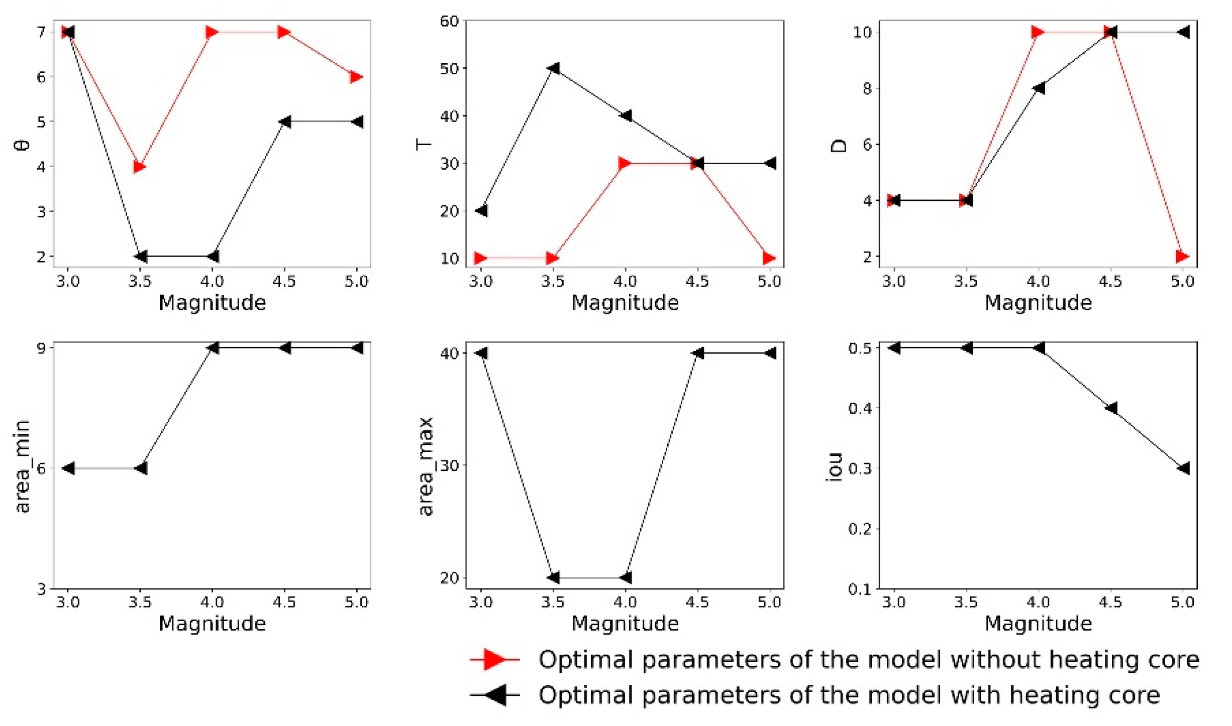
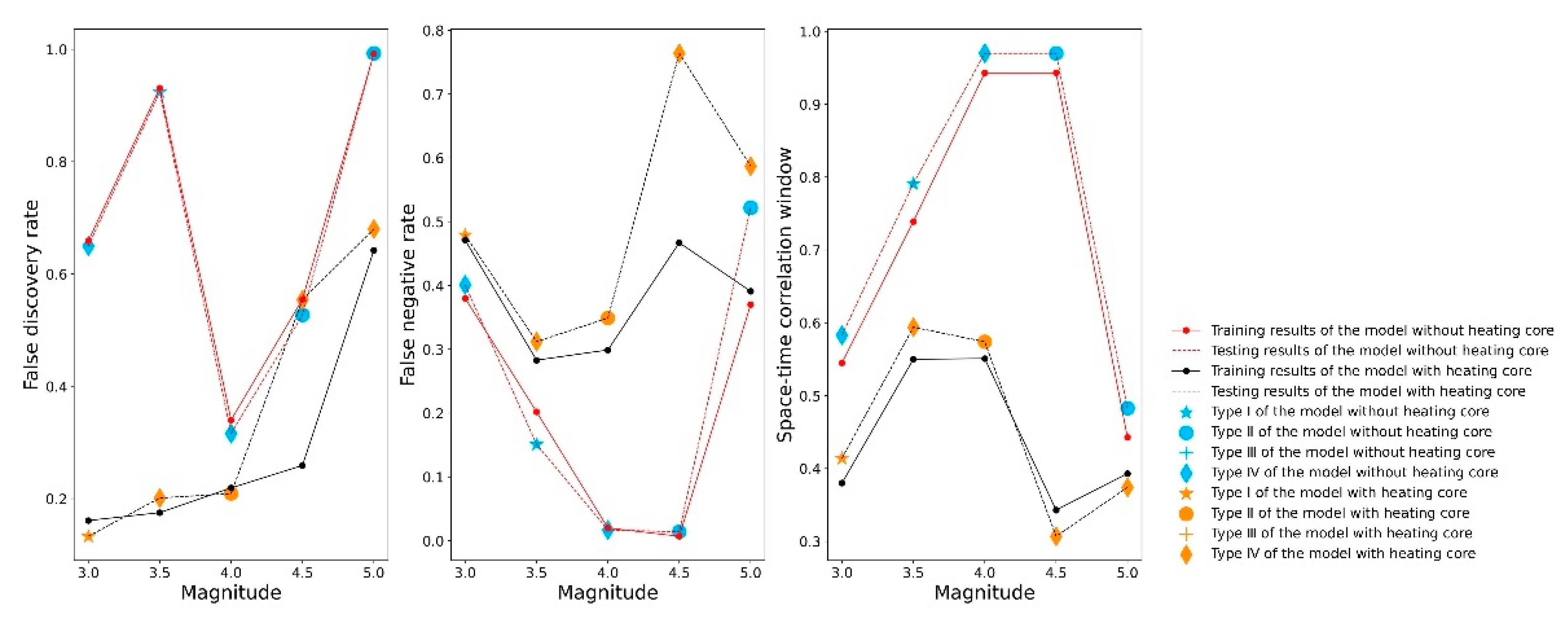
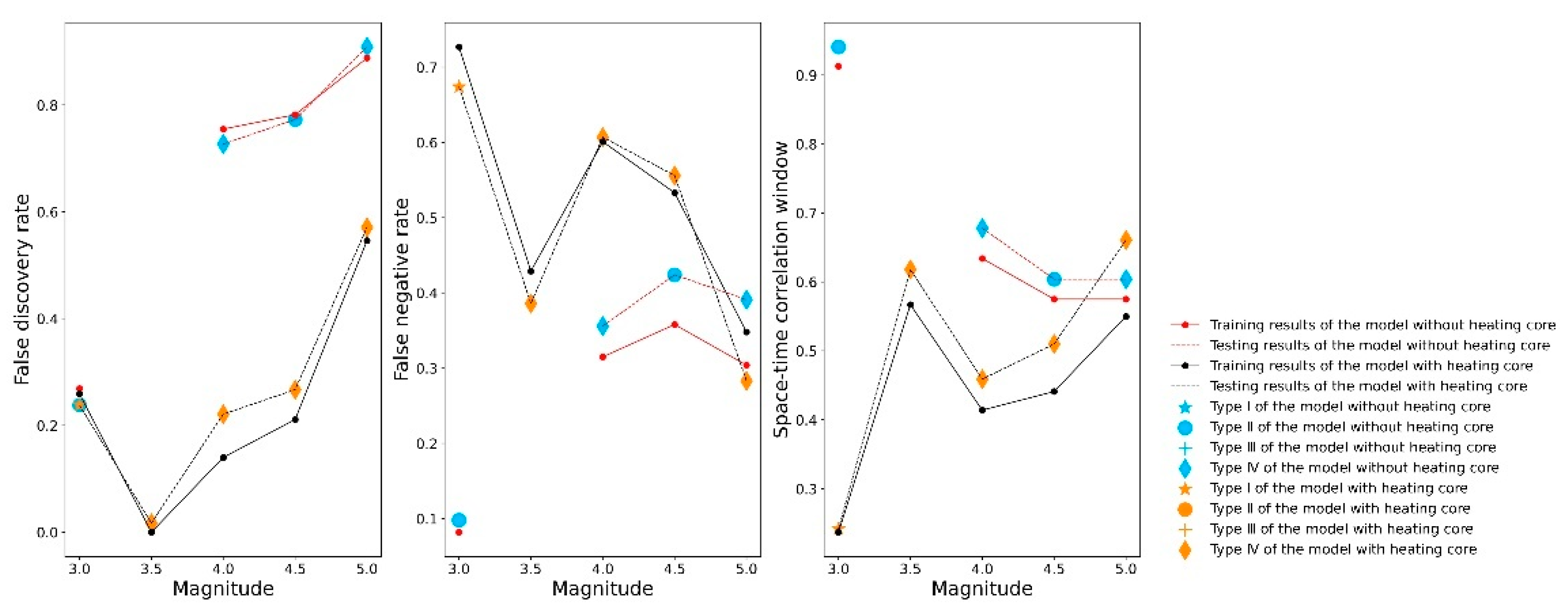
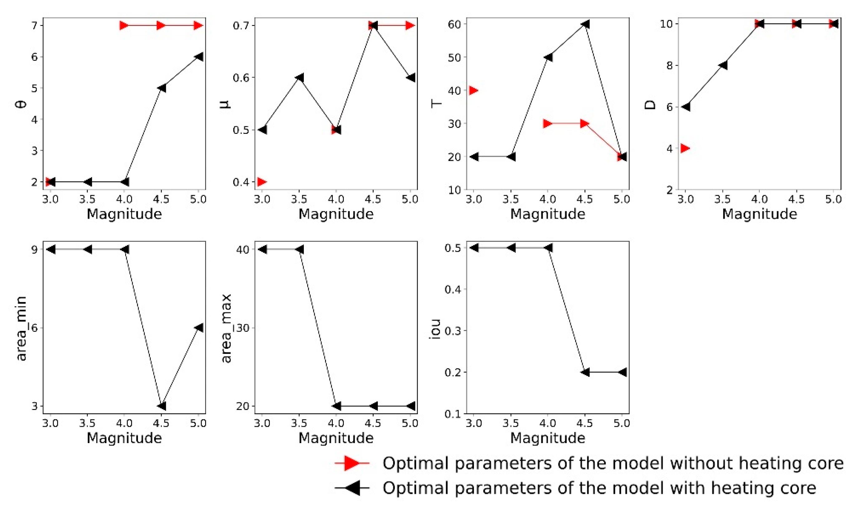
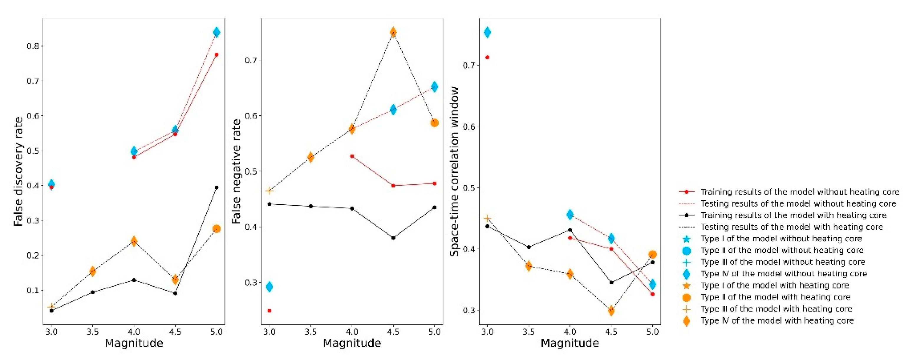
The optimal parameters for the selected models with and without a “heating core” under different magnitudes are shown in Figure 4. The X-axis represents the minimum magnitude parameters—not only for earthquakes with magnitude M—and the other comparative experiments are the same. As shown in Figure 5, under the conditions of five different minimum magnitude parameters, the FDR and STCW of the model with the “heating core” are smaller than those of the model without the “heating core”, indicating that the “heating core” can effectively eliminate thermal noise that is not related to earthquakes and improve the S/N ratio of seismic thermal anomalies. When the minimum magnitude parameter is 3, the test result of the model with the “heating core” is Type I, which is superior to the result of the model without the “heating core”. As the minimum magnitude parameter increases, the FDR of the model with the “heating core” increases, and the type drops to II or IV. Comparing the optimal parameters, it can be seen that the model with the “heating core” sets stricter conditions to reduce the number of alarms and expand the time–space range of the alarm. However, the “heating core” conditions are only valid for the training dataset and lose their effect in the testing dataset.

4.1.2. Comparison with or without a “Heating Core” When the Resampling Scale Is 100

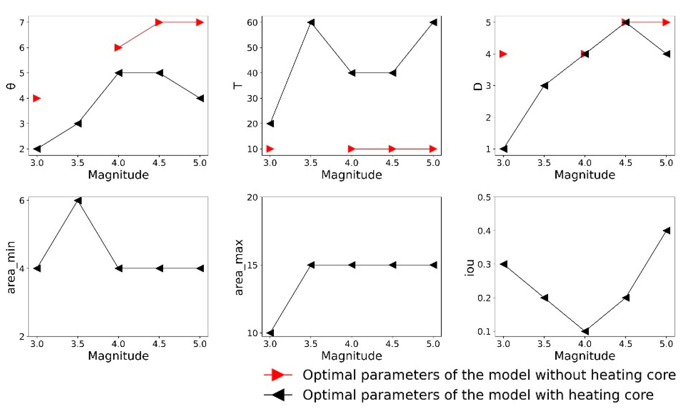
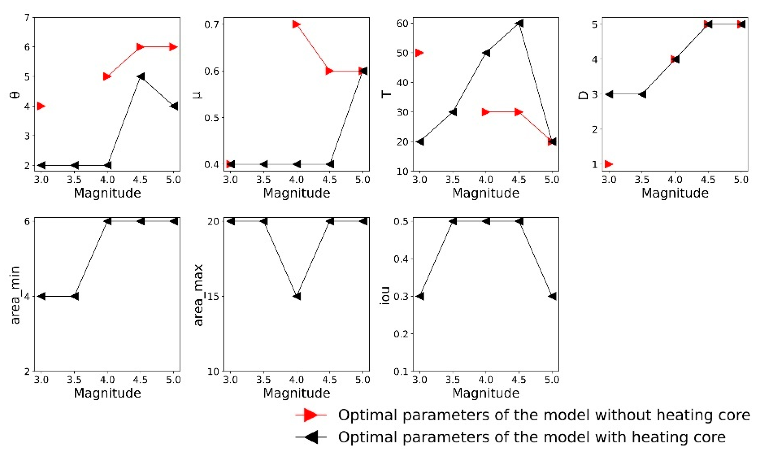
The optimal parameters and the evaluation metrics of the 3D error diagrams under different magnitudes are shown in Figure 6 and Figure 7, respectively. When the minimum magnitude parameter is 3, the test results of the models with and without the “heating core” are superior to those of Type IV, and the test result of the model without the “heating core” (Type II) is superior to random guessing only from the perspective of the FDR. However, the models with a “heating core” are Type I. When the minimum magnitude parameter is 3.5, the model without the “heating core” does not find the optimal parameter in the training data and cannot be effectively predicted. With the increase in the minimum magnitude parameter, the test result of the model with the “heating core” drops to Type IV, while the model without a “heating core” is a Type II when the minimum magnitude parameter is 4.5, but its FDR is higher, meaning that it is not an ideal model.
When the minimum magnitude parameter is 3, the type of the model with the “heating core” in the resampling comparison experiment under the two scales is superior to that of the model without the “heating core”, indicating that the “heating core” filter can effectively eliminate thermal noise that is not related to earthquakes. Therefore, the S/N ratio of seismic thermal anomalies must be improved. However, as the minimum magnitude parameter increases, the models with and without a “heating core” cannot effectively predict earthquakes. From the perspective of the change in the optimal parameters, the model with a “heating core” sets more stringent filter conditions to reduce the number of alarms and expand the warning range of a single alarm. However, this change is only valid in the training dataset, and it performs poorly in the testing dataset.
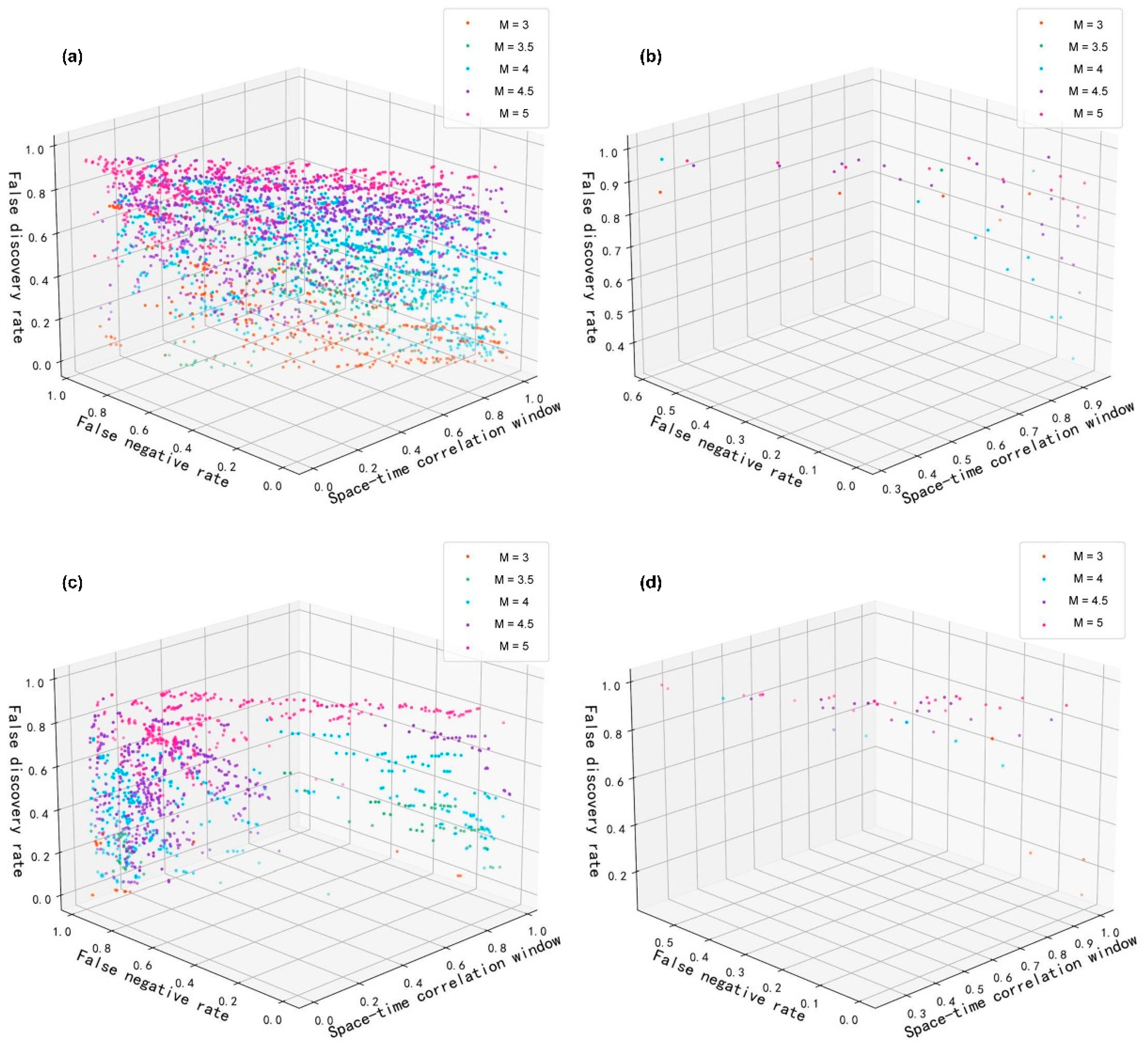
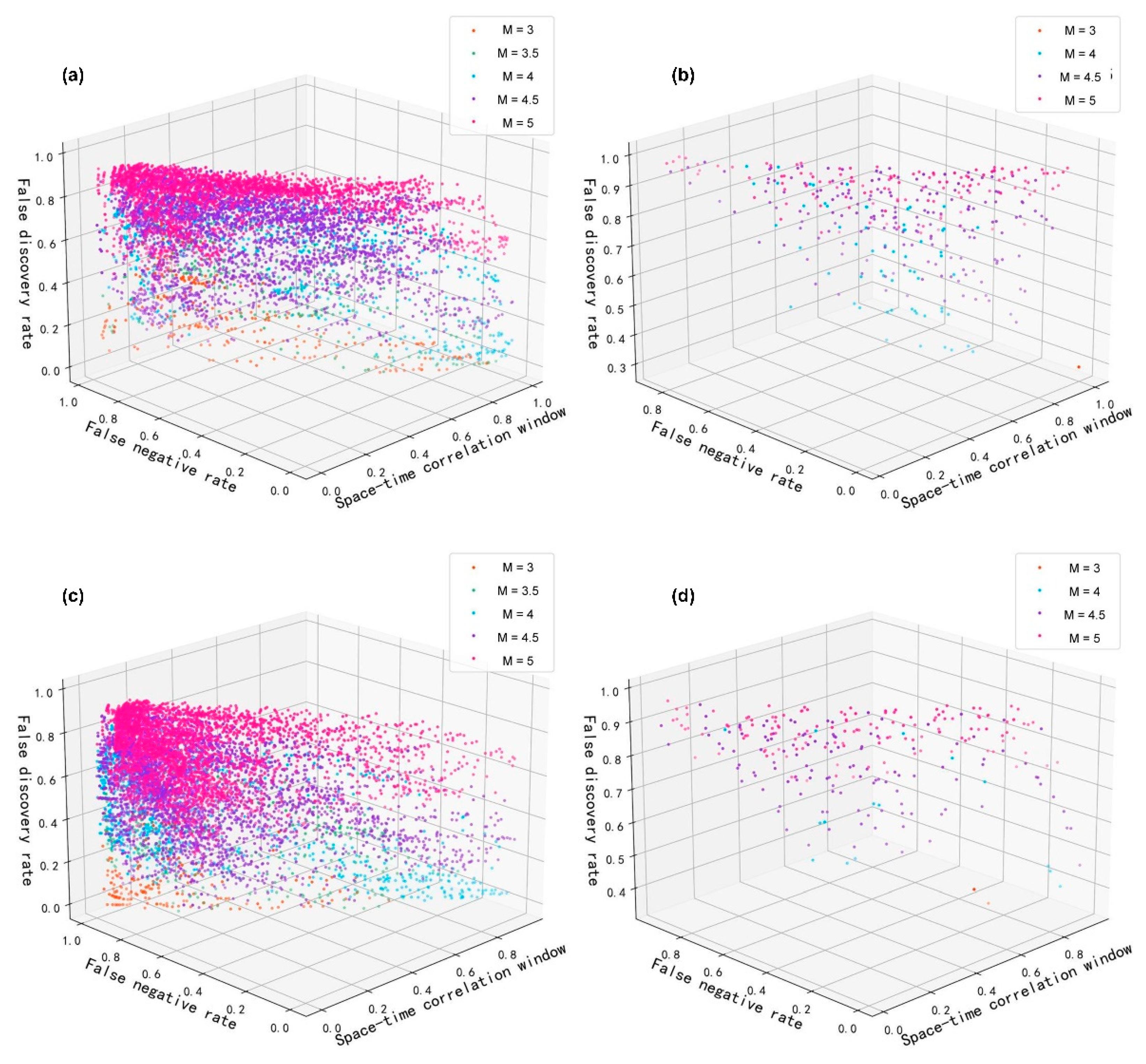
The models with and without a “heating core” in the resampling comparison experiments at the two scales have 40,500 and 900 sets of candidate parameters, respectively. The four 3D error diagrams in Figure 8 indicate the effective parameters that pass the FDR and FNR significance tests under different magnitude parameters simultaneously. The effective parameters in the model without the “heating core” have higher STCW and FDR values in the training dataset. When the TIRA has been filtered by the “heating core”, the FDR of the model is significantly reduced, and the FDR increases with the increase in the minimum magnitude parameter, indicating that the “heating core” filter cannot distinguish the signals of TIRAs generated by earthquakes of different magnitudes and that the FDR for large earthquake predictions is high. In addition, when the resampling scale is 100 km, the effective parameters are concentrated in the region with a higher FNR, and the number of effective parameters is small. When the resampling scale is 50 km, the proportion of effective parameters that pass the significance test is higher. When assigning different weights to the FDR, FNR, or STCW, more effective parameters provide more possibilities for selecting optimal parameters.

4.2. Moving Window

4.2.1. Comparison with or without a “Heating Core” When the Moving Window Size Is 50

The optimal parameters and the evaluation metrics of the 3D error diagrams under different magnitudes are shown in Figure 9 and Figure 10, respectively. When the minimum magnitude parameter is 3.5, the model without a “heating core” does not have the optimal parameters to pass the FNR and FDR significance tests simultaneously during the training step, and it cannot make effective predictions. The model without a “heating core” is Type IV under all four existing magnitude parameters. However, the model with a “heating core” is Type III only when the minimum magnitude parameter is 3, and the test results under other higher magnitude parameters are all Type IV. The number of earthquakes decreases as the magnitude parameter increases, and the parameters θ and μ of the “heating core” model increase. The number of alarms is reduced through stricter filtering conditions, but the FDR in the training and testing datasets still rises. In predicting large earthquakes, the “heating core” filter does not eliminate the thermal anomalies produced by lower-magnitude earthquakes. While reducing the number of alarms, the model with a “heating core” increases the range of spatiotemporal warnings. As with the resampling experiment, the change in this optimal parameter is only valid for the training dataset.

4.2.2. Comparison with or without a “Heating Core” When the Moving Window Size Is 100

As shown in Figure 11, when the magnitude parameter is 3.5, the model without a “heating core” has no optimal parameters in the training dataset, and the test results under other magnitude parameters are all Type IV. The model with a “heating core” is Type III when the minimum magnitude parameter is 3. Similar to the previous experimental results, as the magnitude parameter increases, the “heating core” filter becomes more stringent in filtering suspected thermal anomalies, the number of alarms decreases sharply, and the warning range of a single alarm becomes larger. The model without a “heating core” cannot filter for suspected thermal anomalies, increasing the FDR. As shown in Figure 12, the FDR of the model without a “heating core” is much higher than that of the model with a “heating core”, indicating that the “heating core” at this scale can also eliminate thermal noise that is not related to earthquakes. From the perspective of the FNR, as the minimum magnitude parameter increases—regardless of whether or not the model has a “heating core”—the difference between the results of the training dataset and the results of the testing dataset increases. In particular, when the minimum magnitude parameter is 4, the difference between the training and test results of the “heating core” model is as high as 0.370. This large difference between the training results and the test results indicates that the models with or without a “heating core” have a certain degree of overfitting; that is, the optimal parameters are only applicable to the training dataset, as they perform poorly in the testing dataset.
When the minimum magnitude parameter is 3, the test results of the model with the “heating core” under the two scales of moving window are all Type III, while the model without the “heating core” is Type IV. When the minimum magnitude parameter is 3.5, the model without a “heating core” has no optimal parameters in the training results at either of the two scales. In the moving window comparison experiment, the models with and without a “heating core” have 162,000 and 3600 sets of candidate parameters, respectively. Among them, the effective parameters that pass the FDR and FNR significance tests simultaneously are shown in the 3D error diagram in Figure 13. The FDR of the model without the “heating core” is still higher overall. The distribution of the effective parameters of the model with the “heating core” on the FDR axis is correlated with the magnitude. The FDR of the model with a smaller minimum magnitude parameter is lower and increases with the magnitude of the increase. In addition, the distribution of effective parameters is concentrated in the area with a higher FNR and has no apparent correlation with the magnitude parameter, and this is more obvious when the scale is 100 km.
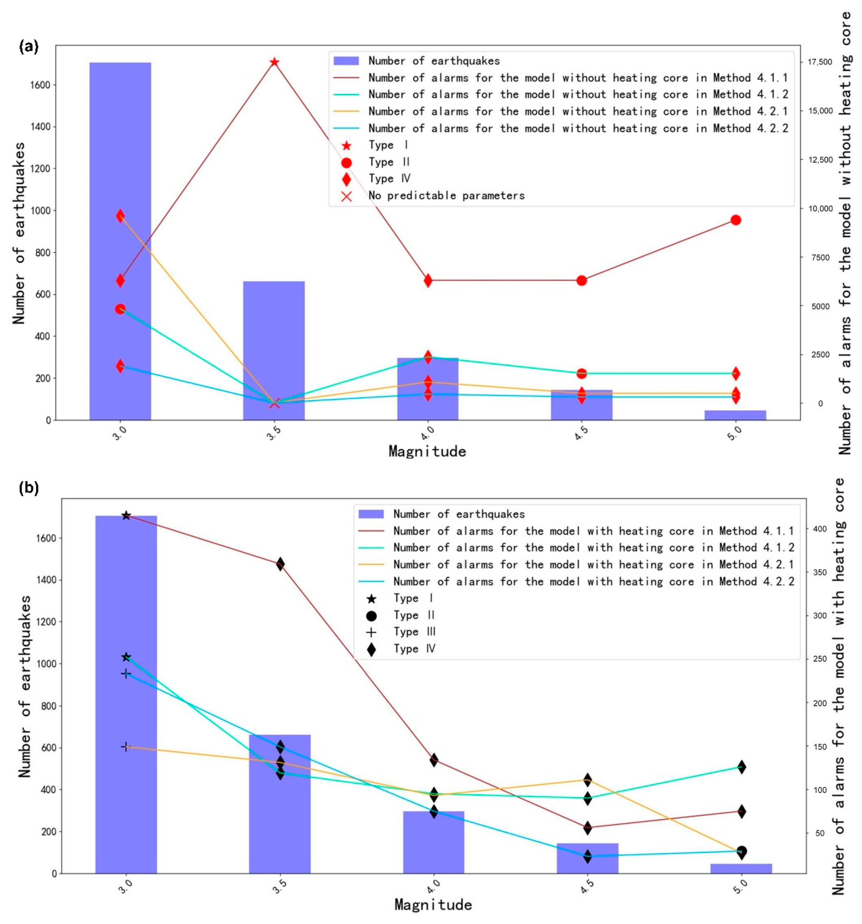
As shown in Figure 14, in earthquake prediction, the number of alarms given by the model with a “heating core” is far lower than that provided by the model without a “heating core”, especially when the magnitude parameter is small; the S/N ratio of seismic thermal anomalies is improved greatly. In the test with a minimum magnitude parameter of 3, the resampling methods at the two scales are both Type I, while the moving window method at the two scales is Type III. The test results of the model without a “heating core” are one Type II alarm and three Type IV alarms. Four sets of comparative experiments show that the model with a “heating core” has superior prediction performance, and the resampling method is superior to the moving-window method. Except for the magnitude parameter of 3, the “heating core” performs poorly under other magnitude parameters; only when the magnitude parameter is 5 and the moving window scale is 100 km does it produce a Type II result, and the rest of the test results are all Type IV. It is worth mentioning that when the magnitude parameter is 3.5, the model without a “heating core” with a resampling scale of 50 km behaves as a Type I, but the number of alarms is as high as 17,502 and the FDR is 92.37%; thus, it is not an excellent model. From this point of view, models with a “heating core” can predict earthquakes of magnitude 3 and above effectively from the perspective of the FDR or FNR, but the prediction of large earthquakes is insufficient.
Theoretically, the frequency of thermal anomalies should be proportional to the frequency of earthquakes if the thermal anomalies are related to earthquakes. Figure 15a,b shows the frequency of thermal anomalies before and after the thermal noise is removed by the “heating core” filter, respectively. The distribution of STIRAs that are not removed by the “heating core” is slightly higher in the northeastern region of the Tibetan Plateau than in the southwestern region, and the overall distribution is relatively even. The frequency of PTIRAs filtered by the “heating core” decreases sharply, showing three main clusters in the northwestern, south–central, and eastern regions, while most of the thermal anomalies in other regions are removed, which is more consistent with the frequency map of earthquake occurrence. This result further indicates that the “heating core” filter greatly improves the S/N ratio of the thermal anomalies.
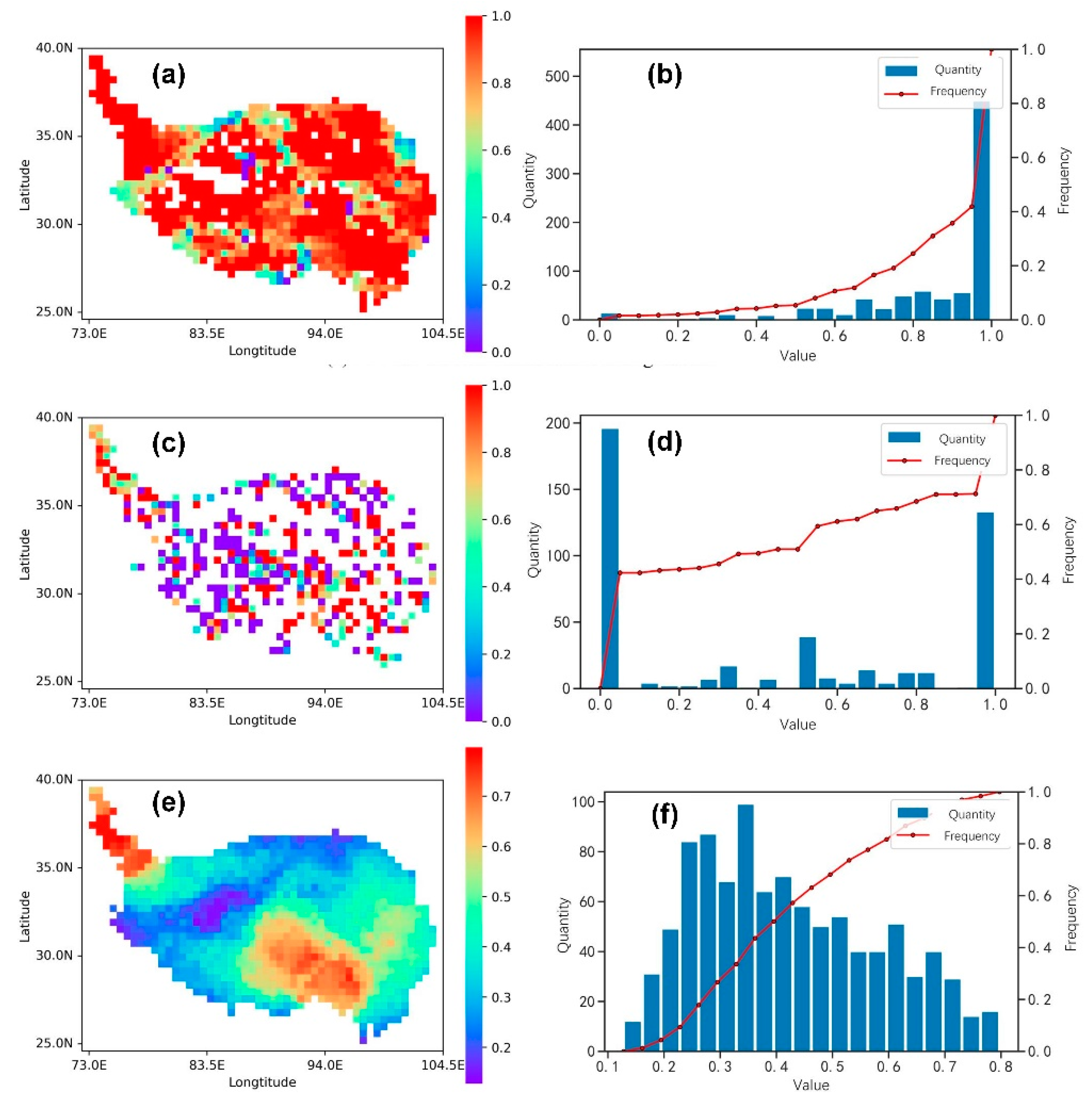
Comparing the four sets of experimental results, we can see that the optimal method to reduce the spatial resolution is the resampling scale of 50 km, the optimal extraction parameters of the STIRAs are ( γ = 50 , θ = 2 ), the optimal parameters of the “heating core” filter are ( a r e a m i n = 6 , a r e a m a x = 40 , i o u = 0.5 ), and the optimal window is ( T = 20 , D = 4 ,   M = 3 ). The spatiotemporal warning range of the optimal binary prediction model is 20 days and 200 km (4 × 50 km), and the PPV in the testing dataset is 86.7%, the TPR is 52.1%, and the STCW is 41.4%. The results of the optimal model in each subregion are shown in Figure 16. The PPV is shown in panel (a), where 63.3% of the regions have a PPV greater than 90%, and 57.3% of the regions have a PPV of 100%. The TPR is shown in panel (b), and the distribution is polarized, with only 29.6% of the regions having a TPR greater than 90% and 42.3% having a TPR of 0. The STCW is shown in panel (c), with two high values in the northwestern and south–central parts of the Tibetan Plateau, with a maximum of 79.7%. In summary, the PPV of the optimal model applies to the whole Qinghai–Tibet Plateau region; however, the TPR is low—especially in the central and western regions, where the STCW is relatively low—and whether or not this is related to the local geological background needs further analysis.

5. Discussion

First, we should discuss the model’s predictive performance with a “heating core” for different earthquake magnitudes. Previous studies have shown that a “heating core” can effectively eliminate non-seismic thermal anomalies [15]. We must acknowledge that researchers have paid extensive attention to earthquake prediction studies in the past. Still, there is currently no research to show whether the thermal anomalies produced by earthquakes of different magnitudes are different. For example, [15,19,20] only consider earthquakes of magnitude 4 and above, neglecting to distinguish between earthquakes of different magnitudes. Our study shows that there is no significant difference in the thermal anomalies produced by different magnitudes under this condition. As shown in Figure 8 and Figure 13, the higher the magnitude parameter M , the higher the FDR corresponding to the effective parameter. Thus, as the magnitude increases, the number of earthquakes decreases, and the “heating core” reduces the number of alarms through more stringent filtering methods to match with earthquakes of higher magnitudes in the training dataset. However, in the testing dataset, these optimal parameters appear to be no different from random guesses. Therefore, the optimal parameters of the “heating core” in the training dataset appear to be overfitted; that is, the “heating core” conditions that are not universally applicable are set according to the higher-magnitude earthquakes in the training dataset, and their performance is poor in the testing dataset. The performance in the prediction of earthquakes with different magnitudes still needs to be explored in further studies.
Second, we should discuss the relationship between the performance of the model and the size of the parameters ( T , D , M ). Counting the number of parameters of the four models with a “heating core” that only pass the FDR test or only pass the FNR test, we found that the frequency of passing the FNR test in the four methods was higher than the frequency of passing the FDR test, as shown in Figure 17. Hence, these models seem to pass the FNR significance test more easily. P2—the average prior probability that the alarm can predict earthquakes successfully—is related to the parameters ( T , D , M ). P2 is positively correlated with the predicted temporal window ( T , D ) and negatively correlated with the earthquake’s predicted magnitude ( M ). Therefore, we recommend that the TD be set as small as possible in the forecasting in order to prevent the model from failing to pass the significance test of the FDR with the large P2.

6. Conclusions

In this study, the TRIMS LST dataset was used to extract thermal anomalies and construct a binary prediction model for earthquakes. To facilitate the statistical analysis and numbering of the thermal anomalies, four sets of experiments were conducted to reduce the spatial resolution of the original data using resampling and moving windows at two scales. The “heating core” filter was also used to remove the noise caused by non-seismic thermal anomalies, and the effects of the “heating core” were compared in each group of experiments. Finally, the optimal prediction model was selected based on the 3D error diagram and the significance test. The results show the following:
(1)
The downscaled spatial resolution method of resampling is superior to the moving-window method, the downscaled spatial resolution scale of 50 km is superior to 100 km, and the “heating core” model with the resampling scale of 50 has the best prediction performance.
(2)
The model with a “heating core” has superior performance compared to the model without a “heating core”, and the “heating core” filter greatly improves the S/N ratio of seismic thermal anomalies. However, the “heating core” is only valid for earthquakes of magnitude 3 and above, and it cannot distinguish the thermal anomalies produced by earthquakes of different magnitudes under this condition.
(3)
For earthquakes of magnitude 3 and above, the test results of the resampling method for the model with the “heating core” under the two scales are all Type I. This model is superior to random guessing from the FNR and FDR perspectives, and the losses are 0.647 (FDR = 13.3%, FNR = 47.9%, STCW = 41.4%) and 0.755 based on the 3D error diagram, respectively; the best model can predict earthquakes effectively within 200 km and within 20 days of a thermal anomaly’s appearance, which can provide a reference for earthquake prediction.
Earthquake prediction is still one of the major scientific questions that need to be explored urgently. The binary prediction model based on thermal infrared anomalies presented in this paper can provide some reference for practical earthquake prediction. In future research on earthquake prediction, hybrid prediction models could be constructed by combining data from thermal anomalies, gas anomalies, and gravitational anomalies in order to improve the performance of the models.

Author Contributions

Conceptualization, C.Z.; Formal analysis, C.Z. and Y.Z.; Methodology, C.Z. and Y.Z.; Software, C.Z.; Supervision, Q.M.; Validation, Q.M.; Visualization, M.A. and X.L.; Writing—draft, C.Z.; Writing—review and editing, Q.M., Y.Z., M.A., L.Z. and P.W. All authors have read and agreed to the published version of the manuscript.

Funding

This research was supported by the National Natural Science Foundation of China Major Program: 42192580, 42192584; the National Natural Science Foundation of China: 42201384; the National Key Research and Development Program of China: 2019YFC1509202; the National Key Research and Development Program of China: 2020YFC0833100.

Institutional Review Board Statement

Not applicable.

Informed Consent Statement

Not applicable.

Acknowledgments

The dataset is provided by the National Tibetan Plateau Data Center (http://data.tpdc.ac.cn, accessed on 20 August 2021).

Conflicts of Interest

The authors declare no conflict of interest.

References

  1. Gornyy, V.; Sal’Man, A.G.; Tronin, A.; Shlin, B.V. The Earth’s Outgoing IR Radiation as an Indicator of Seismic Activity. Proc. Acad. Sci. USSR 1988, 301, 67–69. [Google Scholar]
  2. Freund, F.; Takeuchi, A.; Lau, B.; Hall, C. Positive Holes and Their Role during the Build-up of Stress Prior to the Chi-Chi Earthquake. In Proceedings of the International Conference in Commemoration of 5th Anniversary of the 1999 Chi-Chi Earthquake, Taipei, Taiwan, 8–12 September 2004. [Google Scholar]
  3. Zhu, C.; Jiao, Z.; Shan, X.; Zhang, G.; Li, Y. Land Surface Temperature Variation Following the 2017 Mw 7.3 Iran Earthquake. Remote Sens. 2019, 11, 2411. [Google Scholar] [CrossRef] [Green Version]
  4. Lu, X.; Meng, Q.Y.; Gu, X.F.; Zhang, X.D.; Xie, T.; Geng, F. Thermal Infrared Anomalies Associated with Multi-Year Earthquakes in the Tibet Region Based on China’s FY-2E Satellite Data. Adv. Space Res. 2016, 58, 989–1001. [Google Scholar] [CrossRef]
  5. Zhong, M.; Shan, X.; Zhang, X.; Qu, C.; Guo, X.; Jiao, Z. Thermal Infrared and Ionospheric Anomalies of the 2017 Mw6.5 Jiuzhaigou Earthquake. Remote Sens. 2020, 12, 2843. [Google Scholar] [CrossRef]
  6. Qi, Y.; Wu, L.; Mao, W.; Ding, Y.; He, M. Discriminating Possible Causes of Microwave Brightness Temperature Positive Anomalies Related with May 2008 Wenchuan Earthquake Sequence. IEEE Trans. Geosci. Remote Sens. 2021, 59, 1903–1916. [Google Scholar] [CrossRef]
  7. Pergola, N.; Aliano, C.; Coviello, I.; Filizzola, C.; Genzano, N.; Lacava, T.; Lisi, M.; Mazzeo, G.; Tramutoli, V. Using RST Approach and EOS-MODIS Radiances for Monitoring Seismically Active Regions: A Study on the 6 April 2009 Abruzzo Earthquake. Nat. Hazards Earth Syst. Sci. 2010, 10, 239–249. [Google Scholar] [CrossRef]
  8. Ouzounov, D.; Liu, D.; Chunli, K.; Cervone, G.; Kafatos, M.; Taylor, P. Outgoing Long Wave Radiation Variability from IR Satellite Data Prior to Major Earthquakes. Tectonophysics 2007, 431, 211–220. [Google Scholar] [CrossRef]
  9. Kong, X.; Bi, Y.; Glass, D.H. Detecting Seismic Anomalies in Outgoing Long-Wave Radiation Data. IEEE J. Sel. Top. Appl. Earth Obs. Remote Sens. 2015, 8, 649–660. [Google Scholar] [CrossRef]
  10. Zhang, Y.; Meng, Q.; Wang, Z.; Lu, X.; Hu, D. Temperature Variations in Multiple Air Layers before the Mw 6.2 2014 Ludian Earthquake, Yunnan, China. Remote Sens. 2021, 13, 884. [Google Scholar] [CrossRef]
  11. Khalili, M.; Eskandar, S.S.A.; Panah, S.K.A. Thermal Anomalies Detection before Saravan Earthquake (April 16th, 2013, MW = 7.8) Using Time Series Method, Satellite, and Meteorological Data. J. Earth Syst. Sci. 2020, 129, 5. [Google Scholar] [CrossRef]
  12. Jing, F.; Singh, R.P.; Cui, Y.; Sun, K. Microwave Brightness Temperature Characteristics of Three Strong Earthquakes in Sichuan Province, China. IEEE J. Sel. Top. Appl. Earth Obs. Remote Sens. 2020, 13, 513–522. [Google Scholar] [CrossRef]
  13. Peleli, S.; Kouli, M.; Vallianatos, F. Satellite-Observed Thermal Anomalies and Deformation Patterns Associated to the 2021, Central Crete Seismic Sequence. Remote Sens. 2022, 14, 3413. [Google Scholar] [CrossRef]
  14. Zhang, Y.; Meng, Q. A Statistical Analysis of TIR Anomalies Extracted by RSTs in Relation to an Earthquake in the Sichuan Area Using MODIS LST Data. Nat. Hazards Earth Syst. Sci. 2019, 19, 535–549. [Google Scholar] [CrossRef] [Green Version]
  15. Zhang, Y.; Meng, Q.; Ouillon, G.; Sornette, D.; Ma, W.; Zhang, L.; Zhao, J.; Qi, Y.; Geng, F. Spatially Variable Model for Extracting TIR Anomalies before Earthquakes: Application to Chinese Mainland. Remote Sens. Environ. 2021, 267, 112720. [Google Scholar] [CrossRef]
  16. Fu, C.C.; Lee, L.C.; Ouzounov, D.; Jan, J.C. Earth’s Outgoing Longwave Radiation Variability Prior to M $\geq$6.0 Earthquakes in the Taiwan Area During 2009–2019. Front. Earth Sci. 2020, 8, 364. [Google Scholar] [CrossRef]
  17. Genzano, N.; Filizzola, C.; Hattori, K.; Pergola, N.; Tramutoli, V. Statistical Correlation Analysis Between Thermal Infrared Anomalies Observed from MTSATs and Large Earthquakes Occurred in Japan (2005–2015). J. Geophys. Res. Solid Earth 2021, 126, e2020JB020108. [Google Scholar] [CrossRef]
  18. Zhang, Y.; Meng, Q.; Ouillon, G.; Zhang, L.; Hu, D.; Ma, W.; Sornette, D. Long-Term Statistical Evidence Proving the Correspondence between Tir Anomalies and Earthquakes Is Still Absent. Eur. Phys. J. Spec. Top. 2021, 230, 133–150. [Google Scholar] [CrossRef]
  19. Eleftheriou, A.; Filizzola, C.; Genzano, N.; Lacava, T.; Lisi, M.; Paciello, R.; Pergola, N.; Vallianatos, F.; Tramutoli, V. Long-Term RST Analysis of Anomalous TIR Sequences in Relation with Earthquakes Occurred in Greece in the Period 2004–2013. Pure Appl. Geophys. 2015, 173, 285–303. [Google Scholar] [CrossRef] [Green Version]
  20. Filizzola, C.; Corrado, A.; Genzano, N.; Lisi, M.; Pergola, N.; Colonna, R.; Tramutoli, V. RST Analysis of Anomalous TIR Sequences in Relation with Earthquakes Occurred in Turkey in the Period 2004–2015. Remote Sens. 2022, 14, 381. [Google Scholar] [CrossRef]
  21. Molchan, G.M. Strategies in Strong Earthquake Prediction. Phys. Earth Planet. Inter. 1990, 61, 84–98. [Google Scholar] [CrossRef]
  22. Molchan, G.M. Structure of Optimal Strategies in Earthquake Prediction. Tectonophysics 1991, 193, 267–276. [Google Scholar] [CrossRef]
  23. Swets, J.A. The Relative Operating Characteristic in Psychology. Science 1973, 182, 990–1000. [Google Scholar] [CrossRef] [PubMed]
  24. Zhang, Y.; Guy, O.; Shyam, N.; Didier, S.; Meng, Q. A New 3-D Error Diagram: An Effective and Better Tool for Finding TIR Anomalies Related to Earthquakes. IEEE Trans. Geosci. Remote Sens. under review.
  25. Zechar, J.D.; Jordan, T.H. Testing Alarm-Based Earthquake Predictions. Geophys. J. Int. 2008, 172, 715–724. [Google Scholar] [CrossRef] [Green Version]
  26. Tiampo, K.F.; Rundle, J.B.; McGinnis, S.; Gross, S.J.; Klein, W. Mean-Field Threshold Systems and Phase Dynamics: An Application to Earthquake Fault Systems. Europhys. Lett. EPL 2002, 60, 481–488. [Google Scholar] [CrossRef]
  27. DeVries, P.M.R.; Viégas, F.; Wattenberg, M.; Meade, B.J. Deep Learning of Aftershock Patterns Following Large Earthquakes. Nature 2018, 560, 632–634. [Google Scholar] [CrossRef]
  28. Mignan, A.; Broccardo, M. One Neuron versus Deep Learning in Aftershock Prediction. Nature 2019, 574, E1–E3. [Google Scholar] [CrossRef] [Green Version]
  29. Yousefzadeh, M. Spatiotemporally Explicit Earthquake Prediction Using Deep Neural Network. Soil Dyn. Earthq. Eng. 2021, 11, 106663. [Google Scholar] [CrossRef]
  30. Wang, Q.; Guo, Y.; Yu, L.; Li, P. Earthquake Prediction Based on Spatio-Temporal Data Mining: An LSTM Network Approach. IEEE Trans. Emerg. Top. Comput. 2020, 8, 148–158. [Google Scholar] [CrossRef]
  31. Berhich, A.; Belouadha, F.Z.; Kabbaj, M.I. LSTM-Based Models for Earthquake Prediction. In Proceedings of the 3rd International Conference on Networking, Information Systems & Security, Marrakech, Morocco, 31 March–2 April 2020; ACM: Marrakech, Morocco, 2020; pp. 1–7. [Google Scholar]
  32. Banna, M.d.H.A.; Ghosh, T.; Nahian, M.d.J.A.; Taher, K.A.; Kaiser, M.S.; Mahmud, M.; Hossain, M.S.; Andersson, K. Attention-Based Bi-Directional Long-Short Term Memory Network for Earthquake Prediction. IEEE Access 2021, 9, 56589–56603. [Google Scholar] [CrossRef]
  33. Shodiq, M.N.; Kusuma, D.H.; Rifqi, M.G.; Barakbah, A.R.; Harsono, T. Adaptive Neural Fuzzy Inference System and Automatic Clustering for Earthquake Prediction in Indonesia. JOIV Int. J. Inform. Vis. 2019, 3, 47–53. [Google Scholar] [CrossRef] [Green Version]
  34. Jiang, C.; Wei, X.; Cui, X.; You, D. Application of Support Vector Machine to Synthetic Earthquake Prediction. Earthq. Sci. 2009, 22, 315–320. [Google Scholar] [CrossRef]
  35. Parsons, T. On the Use of Receiver Operating Characteristic Tests for Evaluating Spatial Earthquake Forecasts. Geophys. Res. Lett. 2020, 47, e2020GL088570. [Google Scholar] [CrossRef]
  36. Blackett, M.; Wooster, M.J.; Malamud, B.D. Exploring Land Surface Temperature Earthquake Precursors: A Focus on the Gujarat (India) Earthquake of 2001. Geophys. Res. Lett. 2011, 38. [Google Scholar] [CrossRef]
  37. Meng, Q.; Zhang, Y. Discovery of Spatial-Temporal Causal Interactions between Thermal and Methane Anomalies Associated with the Wenchuan Earthquake. Eur. Phys. J. Spec. Top. 2021, 230, 247–261. [Google Scholar] [CrossRef]
  38. Weiyu, M.; Xuedong, Z.; Liu, J.; Yao, Q.; Zhou, B.; Yue, C.; Kang, C.; Lu, X. Influences of Multiple Layers of Air Temperature Differences on Tidal Forces and Tectonic Stress before, during and after the Jiujiang Earthquake. Remote Sens. Environ. 2018, 210, 159–165. [Google Scholar] [CrossRef]
  39. Genzano, N.; Filizzola, C.; Paciello, R.; Pergola, N.; Tramutoli, V. Robust Satellite Techniques (RST) for Monitoring Earthquake Prone Areas by Satellite TIR Observations: The Case of 1999 Chi-Chi Earthquake (Taiwan). J. Asian Earth Sci. 2015, 114, 289–298. [Google Scholar] [CrossRef]
  40. Genzano, N.; Filizzola, C.; Lisi, M.; Pergola, N.; Tramutoli, V. Toward the Development of a Multi Parametric System for a Short-Term Assessment of the Seismic Hazard in Italy. Ann. Geophys. 2020, 63, PA550. [Google Scholar] [CrossRef]
  41. Blum, M.; Lensky, I.M.; Nestel, D. Estimation of Olive Grove Canopy Temperature from MODIS Thermal Imagery Is More Accurate than Interpolation from Meteorological Stations. Agric. For. Meteorol. 2013, 176, 90–93. [Google Scholar] [CrossRef]
  42. Wan, Z.; Zhang, Y.; Zhang, Q.; Li, Z.L. Quality Assessment and Validation of the MODIS Global Land Surface Temperature. Int. J. Remote Sens. 2004, 25, 261–274. [Google Scholar] [CrossRef]
  43. Zhang, X.; Peng, L.; Zheng, D.; Tao, J. Cloudiness Variations over the Qinghai-Tibet Plateau during 1971–2004. J. Geogr. Sci. 2008, 18, 142–154. [Google Scholar] [CrossRef]
  44. Zhou, J.; Zhang, X.; Zhan, W.; Gottsche, F.M.; Liu, S.; Olesen, F.S.; Hu, W.; Dai, F. A Thermal Sampling Depth Correction Method for Land Surface Temperature Estimation from Satellite Passive Microwave Observation Over Barren Land. IEEE Trans. Geosci. Remote Sens. 2017, 55, 4743–4756. [Google Scholar] [CrossRef]
  45. Zhang, X.; Zhou, J.; Gottsche, F.M.; Zhan, W.; Liu, S.; Cao, R. A Method Based on Temporal Component Decomposition for Estimating 1-Km All-Weather Land Surface Temperature by Merging Satellite Thermal Infrared and Passive Microwave Observations. IEEE Trans. Geosci. Remote Sens. 2019, 57, 4670–4691. [Google Scholar] [CrossRef]
  46. Zhang, X.; Zhou, J.; Liang, S.; Wang, D. A Practical Reanalysis Data and Thermal Infrared Remote Sensing Data Merging (RTM) Method for Reconstruction of a 1-Km All-Weather Land Surface Temperature. Remote Sens. Environ. 2021, 260, 112437. [Google Scholar] [CrossRef]
  47. Tang, W.; Zhou, J.; Zhang, X.; Zhang, X.; Ma, J.; Ding, L. Daily 1-Km All-Weather Land Surface Temperature Dataset for the Chinese Landmass and Its Surrounding Areas (TRIMS LST.; 2000–2020); National Tibetan Plateau Data Center: Beijing, China, 2021. [Google Scholar] [CrossRef]
  48. Žalohar, J. Gutenberg-Richter’s Law. In Developments in Structural Geology and Tectonics; Elsevier: Amsterdam, The Netherlands, 2018; pp. 173–178. [Google Scholar]
  49. Ellsworth, W.L.; Fatih, B. Nucleation of the 1999 Izmit Earthquake by a Triggered Cascade of Foreshocks. Nat. Geosci. 2018, 11, 531–535. [Google Scholar] [CrossRef]
  50. Helmstetter, A.; Sornette, D.; Grasso, J.R. Mainshocks Are Aftershocks of Conditional Foreshocks: How Do Foreshock Statistical Properties Emerge from Aftershock Laws: Mainshocks are Aftershocks of Conditional Foreshocks. J. Geophys. Res. Solid Earth 2003, 108. [Google Scholar] [CrossRef] [Green Version]
  51. Bouchon, M.; Durand, V.; Marsan, D.; Karabulut, H.; Schmittbuhl, J. The Long Precursory Phase of Most Large Interplate Earthquakes. Nat. Geosci. 2013, 6, 299–302. [Google Scholar] [CrossRef]
  52. Carl, T.; Stephen, H.; Vipul, S.; Jessica, H.; Yoshihiro, K.; Paul, A.J.; Chen, J.; Natalia, R.; Kyle, S.; West, M.E. Earthquake Nucleation and Fault Slip Complexity in the Lower Crust of Central Alaska. Nat. Geosci. 2018, 11, 536–541. [Google Scholar]
  53. Tormann, T.; Enescu, B.; Woessner, J.; Wiemer, S. Randomness of Megathrust Earthquakes Impliedby Rapid Stress Recovery after the Japanearthquake. Nat. Geosci. 2015, 8, 152–158. [Google Scholar] [CrossRef]
  54. Zhang, Y. Earthquake Forecasting Model Based on the Thermal Infrared Anomalies for Chinese Mainland. Ph.D. Thesis, University of Chinese Academy of Sciences, Huairou District, China, 2021. [Google Scholar]
  55. Gardner, J.K.; Knopoff, L. Is the Sequence of Earthquakes in Southern California, with Aftershocks Removed, Poissonian? Bull. Seismol. Soc. Am. 1974, 64, 1363–1367. [Google Scholar] [CrossRef]
  56. Knopoff, L. The Statistics of Earthquakes in Southern California. Seismol. Soc. Am. 1964, 54, 1871–1873. [Google Scholar] [CrossRef]
  57. Knopoff, L.; Gardner, J.K. Higher Seismic Activity During Local Night on the Raw Worldwide Earthquake Catalogue. Geophys. J. R. Astron. Soc. 2010, 28, 311–313. [Google Scholar] [CrossRef]
  58. Reasenberg, P. Second-Order Moment of Central California Seismicity, 1969–1982. J. Geophys. Res. 1985, 90, 5479–5495. [Google Scholar] [CrossRef]
  59. Frohlich, C.; Davis, S.D. Single-Link Cluster Analysis as A Method to Evaluate Spatial and Temporal Properties of Earthquake Catalogues. Geophys. J. Int. 1990, 100, 19–32. [Google Scholar] [CrossRef] [Green Version]
  60. Zaliapin, I.; Gabrielov, A.; Keilis-Borok, V.; Wong, H. Clustering Analysis of Seismicity and Aftershock Identification. Phys. Rev. Lett 2008, 101, 018501. [Google Scholar] [CrossRef] [Green Version]
  61. Baiesi, M.; Paczuski, M. Scale Free Networks of Earthquakes and Aftershocks. Phys. Rev. E 2004, 69, 066106. [Google Scholar] [CrossRef]
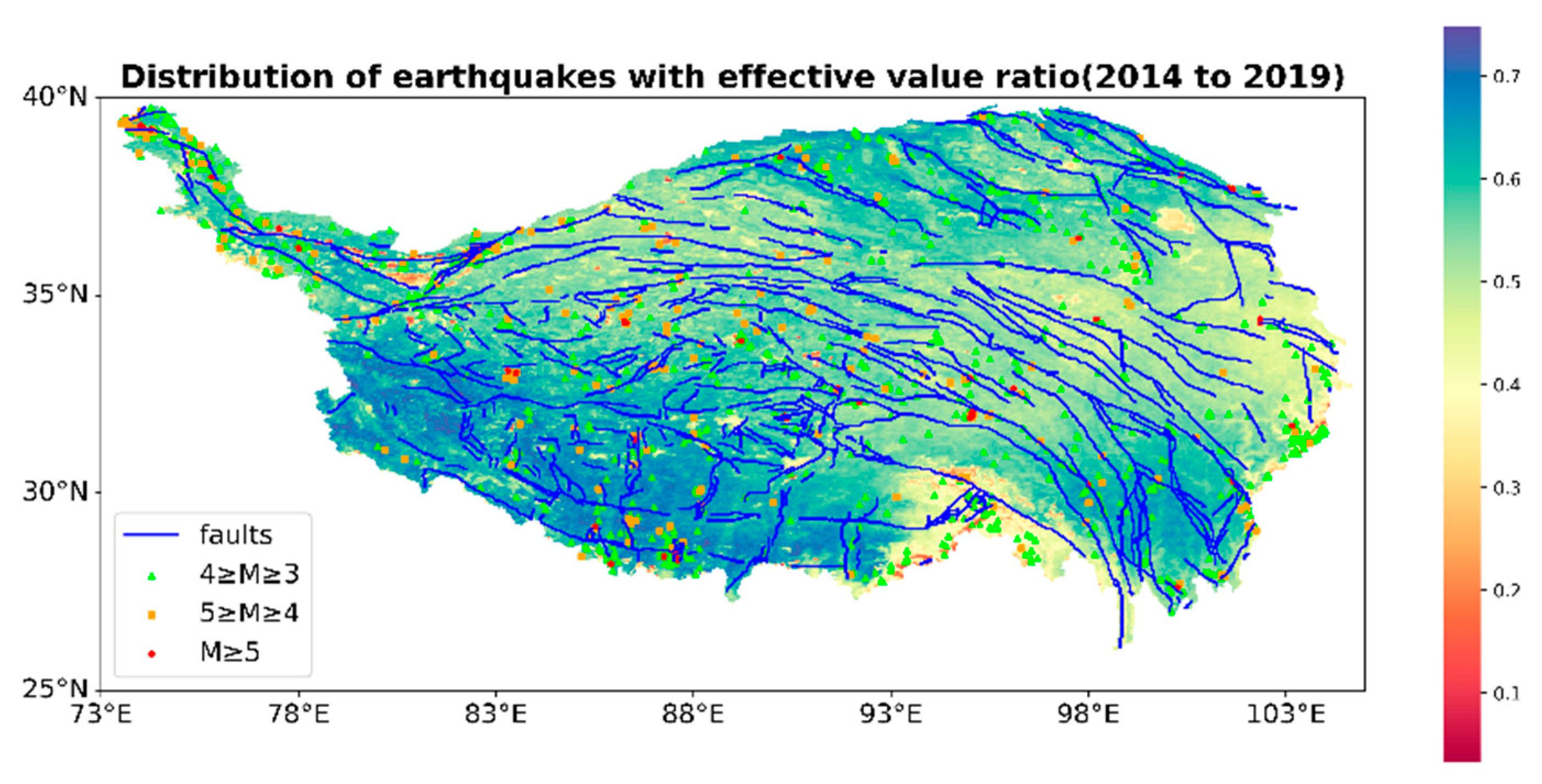
Figure 1. The spatial distribution of earthquakes and faults from 2014 to 2019. The note on the right indicates the frequency of pixels not covered by clouds of the raw TIR data in the selected period.
Remotesensing 14 05925 g001
Figure 2. (a) The number of earthquakes that occurred from 2010 to 2019; affected by the 2008 Wenchuan earthquake, the frequency of earthquakes in that year increased significantly. (b) The completeness examination of the earthquake catalog.
Remotesensing 14 05925 g002
Figure 3. Experimental flowchart of this research.
Remotesensing 14 05925 g003
Figure 4. The optimal parameters of the models with/without the “heating core” when the resampling scale is 50 under different magnitude parameters; the red line indicates the change in the optimal parameters of the model without a “heating core”, while the black line indicates the change in the optimal parameters of the model with a “heating core” (the same below).
Remotesensing 14 05925 g004
Figure 5. Comparison of the training and test results of the optimal model with and without a “heating core” at different magnitudes when the resampling scale is 50; the solid line and the dashed line represent the results of training and testing, respectively, while the blue and yellow marks represent the alarm types of the models without/with a “heating core”, respectively (the same below).
Remotesensing 14 05925 g005
Figure 6. The optimal parameters of the models with/without a “heating core” when the resampling scale is 100 under different magnitude parameters.
Remotesensing 14 05925 g006
Figure 7. Comparison of the training and test results of the optimal models with/without a “heating core” at different magnitudes when the resampling scale is 100.
Remotesensing 14 05925 g007
Figure 8. Comparison of the results of resampling experiments for parameters that pass the significance tests of FNR and FDR simultaneously under different magnitude parameters: (a) the model with a “heating core” when the resampling scale is 50, where a total of 3459 sets of parameters pass the test; (b) the model without a “heating core” when the resampling scale is 50, where a total of 50 sets of parameters pass the test; (c) the model with a “heating core” when the resampling scale is 100, where a total of 1337 sets of parameters pass the test; (d) the model without a “heating core” when the resampling scale is 100, where a total of 48 sets of parameters pass the test.
Remotesensing 14 05925 g008
Figure 9. The optimal parameters of the models with/without a “heating core” when the moving window size is 50 under different magnitude parameters.
Remotesensing 14 05925 g009
Figure 10. Comparison of the training and test results of the optimal models with and without a “heating core” at different magnitudes when the moving window size is 50.
Remotesensing 14 05925 g010
Figure 11. The optimal parameters of the models with/without a “heating core” when the moving window scale is 100 under different magnitude parameters.
Remotesensing 14 05925 g011
Figure 12. Comparison of the training and test results of the optimal models with and without a “heating core” at different magnitudes when the moving window scale is 100.
Remotesensing 14 05925 g012
Figure 13. Moving windows comparing the results of the parameters that pass the significance test of the FDR and FNR simultaneously under different magnitude parameters in the experiments: (a) the model with a “heating core” when the moving window scale is 50 km, where a total of 7005 sets of parameters pass the test; (b) the model without a “heating core” when the moving window scale is 50 km, where a total of 355 sets of parameters pass the test; (c) the model with a “heating core” when the moving window scale is 100 km, where a total of 8421 sets of parameters pass the test; (d) the model without a “heating core” when the moving window scale is 100 km, where a total of 272 sets of parameters pass the test.
Remotesensing 14 05925 g013
Figure 14. The models with and without a “heating core” respond to different magnitude parameters in the four methods: (a) the model without a “heating core”; (b) the model with a “heating core”.
Remotesensing 14 05925 g014
Figure 15. (a) The frequency of STIRAs in the testing dataset; (b) the frequency of PTIRAs in the testing dataset; (c) the frequency of earthquakes in the testing dataset.
Remotesensing 14 05925 g015
Figure 16. The results for the best spatially variable parameters of the testing dataset: (a,b) the PPV of the optimal model in each subregion and the distribution histogram of the PPV, respectively; (c,d) the TPR of the optimal model in each subregion and the distribution histogram of the TPR, respectively; (e,f) the STCW of the optimal model in each subregion and the distribution histogram of the STCW, respectively. The white pixels represent values for each subregion that were not involved in the calculation using the testing dataset.
Remotesensing 14 05925 g016
Figure 17. The relationship between P2 and the FDR, where P2 represents the average prior probability that all alarms can successfully predict an earthquake: (a,b) represents the results when the resampling window scale is 50 km and 100 km, respectively; (c,d) the results when the moving window scale is 50 km and 100 km, respectively.
Remotesensing 14 05925 g017
Table 1. Conditions for the classification of alarm types.
TypeCondition
IP1 ≤ 0.05 and P2 ≤ 0.05
IIP1 ≥ 0.05 and P2 ≤ 0.05
IIIP1 ≤ 0.05 and P2 ≥ 0.05
IVP1 ≥ 0.05 and P2 ≥ 0.05
Table 2. Candidate parameters for models with/without a “heating core” when the resampling scale is 50.
ParameterHeating CoreValue
γ Yes/No50 (km)
θ Yes/No2, 3, 4, 5, 6, 7 (K)
a r e a m i n Yes3, 6, 9 (50 km × 50 km)
a r e a m a x Yes20, 30, 40 (50 km × 50 km)
i o u Yes0.1, 0.2, 0.3, 0.4, 0.5
T Yes/No10, 20, 30, 40, 50, 60 (days)
D Yes/No2, 4, 6, 8, 10 (50 km)
M Yes/No3, 3.5, 4, 4.5, 5
Table 3. Candidate parameters for models with/without a “heating core” when the resampling scale is 100.
ParameterHeating CoreValue
γ Yes/No100 (km)
θ Yes/No2, 3, 4, 5, 6, 7 (K)
a r e a m i n Yes2, 4, 6 (100 km × 100 km)
a r e a m a x Yes10, 15, 20 (100 km × 100 km)
i o u Yes0.1, 0.2, 0.3, 0.4, 0.5
T Yes/No10, 20, 30, 40, 50, 60 (day)
D Yes/No1, 2, 3, 4, 5 (100 km)
M Yes/No3, 3.5, 4, 4.5, 5
Table 4. Candidate parameters for models with and without a “heating core” when the moving window scale is 50.
ParameterHeating CoreValue
s Yes/No50 (km)
μ Yes/No0.4, 0.5, 0.6, 0.7
θ Yes/No2, 3, 4, 5, 6, 7 (K)
a r e a m i n Yes3, 6, 9 (50 km × 50 km)
a r e a m a x Yes20, 30, 40 (50 km × 50 km)
i o u Yes0.1, 0.2, 0.3, 0.4, 0.5
T Yes/No10, 20, 30, 40, 50, 60 (day)
D Yes/No2, 4, 6, 8, 10 (50 km)
M Yes/No3, 3.5, 4, 4.5, 5
Table 5. Candidate parameters for models with and without a “heating core” when the moving window scale is 100.
ParameterHeating CoreValue
s Yes/No100 (km)
μ Yes/No0.4, 0.5, 0.6, 0.7
θ Yes/No2, 3, 4, 5, 6, 7 (K)
a r e a m i n Yes2, 4, 6 (100 km × 100 km)
a r e a m a x Yes10, 15, 20 (100 km × 100 km)
i o u Yes0.1, 0.2, 0.3, 0.4, 0.5
T Yes/No10, 20, 30, 40, 50, 60 (day)
D Yes/No1, 2, 3, 4, 5 (100 km)
M Yes/No3, 3.5, 4, 4.5, 5
Publisher’s Note: MDPI stays neutral with regard to jurisdictional claims in published maps and institutional affiliations.